Optimization of emergency frequency control strategy for power systems considering both source and load uncertainties

With the increasing integration of renewable energy sources and the presence of numerous controllable loads such as electric vehicles and energy storage in the modern power system, higher nonlinearities and uncertainty both sources and loads are introduced. These factors pose challenges in achieving fast and accurate emergency frequency control. Therefore, this paper addresses the issue of dual source-load uncertainties in power system and presents an optimization strategy based on the Soft Actor Critic (SAC) algorithm that involves the participation of controllable loads in emergency frequency control. Firstly, the spatio-temporal uncertainties of wind farm power output on power supply side and power demand on the load side are described using Weibull and normal probability distributions, respectively. Secondly, an improved Markov Decision Process (MDP) model for emergency frequency control is established, which considers the characteristics of the dual source-load uncertainties. Finally, an optimization of the SAC algorithm is conducted based on Deep Reinforcement Learning (DRL), aiming to achieve rapid system frequency recovery and minimize the cost of removing controllable loads. The presented approach in the paper enhances the emergency frequency control strategy for uncertain power systems and effectively addresses the issue of source-load uncertainty compounded by fault power shortages.

1 Introduction

The modern power system is continuously evolving and advancing, characterized by sustainability, distribution, dynamism, and intelligent openness. As a result, the control strategy ensuring frequency security and stability in power system has become increasingly complex, leading to greater challenges in emergency frequency control (Zhou et al., 2018; Yi et al., 2019; Li et al., 2020). Meanwhile, the power supply side in power system appears an increasing penetration rate of renewable energy sources. Additionally, there is a significant number of new controllable loads with significant power fluctuations on the load side. These introduce double uncertainties on both the sources and load sides, exacerbating the power shortfalls that occur during system disturbances and further increasing the complexity of accidents. Hence, it holds immense importance to investigate the emergency frequency control of power system characterized by dual source and load uncertainties.

Considering the nonlinearities and uncertainties at both power supply and load side in modern power systems, various approaches have been proposed to optimize emergency frequency stabilization control, including adaptive and semi-adaptive Under-Frequency Load Shedding (UFLS) methods, event-driven load shedding methods (Xue et al., 2014; Li et al., 2017; Cao et al., 2021), and strategies addressing low inertial (Wu et al., 2015). An emergency frequency control strategy that involves the collaborative participation of renewable energy field stations and conventional units to ensure frequency stabilization while minimizing control costs is conducted (Ke et al., 2022). Reference (Chandra and Pradhan, 2020) addresses an adaptive emergency load shedding method incorporating synchronous generator and photovoltaic plant equivalent models that consider the stochastic variation of solar PV plant power. Frequency characteristics of systems with high penetration of advanced energy technologies is analyzed and proposes a low-frequency load shedding blocking optimization strategy based on df/dt (Sheng et al., 2021). Reference (Masood et al., 2021) presents an emergency frequency stabilization control that simultaneously ensures voltage stability for low-inertia power system containing numerous wind turbines. Reference (Wang et al., 2019) investigates an adaptive emergency frequency control scheme based on inertia estimation from load measurement information of high-percentage renewable energy system. The uncertainty of wind power output and effect of frequency regulation are considered (Zhou and Shi, 2021), an emergency frequency control strategy that combines high-frequency cut-off and low-frequency load-shedding measures are optimized by considering the frequency confidence of power system.

The optimization of emergency frequency control mentioned above primarily adopts model-based methods, including the time-domain simulation method, the dynamic equivalence method, and the linearization analysis method (Zhang et al., 2009; Liu et al., 2014). Among these, the time-domain simulation method is time-consuming and computationally intensive, although it has high accuracy. The dynamic equivalence method is computationally efficient but has low accuracy, which does not meet the requirements of actual power grid. The linearized analysis combines the advantages of the former two methods (Larik et al., 2018), but it does not adapt the topology changes and new elements of power grid. Due to the limitations of physical models, the approaches based on physical models cannot fit with the development of power grid.

In recent years, Machine Learning (ML) methods have been increasingly applied to power system stability control. These methods are based on data for feature mining, do not require accurate mathematical models, and have significant computational performance advantages. Reference (Dai et al., 2012) trained a load shedding prediction model offline using an extreme learning machine and achieved online prediction of actual load shedding. In reference (Bai et al., 2016), an artificial neural network RBF-ANN model was employed to estimate and predict the frequency dynamics process of the power system, contributing to the development of an emergency frequency control scheme. Despite their fast computational speed, traditional ML algorithms are considered shallow learning methods, often relying heavily on expert experience. Their control effectiveness is influenced by the size and quality of the database, resulting in limited adaptability in achieving desired control outcomes. The advancements in deep learning have garnered attention due to their impressive training effectiveness. Consequently, several scholars have explored the application of deep learning methods in optimizing emergency control strategies for power systems (Hu et al., 2019; Lin, 2022). These methods simultaneously enhance control accuracy and reduce decision-making time. In Reference (Qiang et al., 2022), an emergency control model based on an enhanced AlexNet convolutional network is established. This model predicts the system’s emergency control sensitivity and identifies alternative control buses, ultimately optimizing to obtain the emergency control strategy. However, deep learning methods require a large number of datasets for model training. In high-dimensional action space problems, a multitude of control scenarios emerge, leading to a significant volume of invalid datasets. This abundance of data presents challenges in model training.

The DRL technique combines the advantages of deep learning and reinforcement learning, which can realize high-dimensional feature extraction and direct learning of complex action space. Hence, to address the highly nonlinear and uncertain nature of emergency frequency stability control problems, some researchers have employed DRL algorithms to optimize strategies that enhance frequency stability while minimizing the total amount of load shedding (Yang et al., 2022). Reference (Chen et al., 2020) optimizes the emergency frequency control strategy using DRL algorithms to reduce frequency stability fluctuations. However, the state space considered in this approach focuses solely on the frequency deviation of the center of inertia. This limitation may lead to inaccurate outcomes since system topology and parameters can significantly vary across different scenarios. In Reference (Ma et al., 2020), a distributed reinforcement learning algorithm is utilized to optimize the emergency frequency control strategy, resulting in improved computational performance and robustness. Reference (Xie and Sun, 2022) considered load variations, measurement noise, and communication delays in real power systems by proposing an emergency frequency control method based on a distributed Soft Actor Critic (SAC) algorithm.

In this paper, a controllable load participation emergency frequency optimization control strategy for source-load dual uncertainty power systems is proposed based on deep reinforcement learning SAC algorithm to address the above problems. Firstly, the source-side output spatio-temporal uncertainty and load-side power uncertainty are described by Weibull and normal probability distribution. Secondly, the action space, state space and reward function of the MDP model are improved according to the characteristics of source-load uncertainty. Then the deep reinforcement learning SAC algorithm with continuous action space is used to train the model to obtain an emergency frequency optimization control strategy for the dual source-load uncertainty power system, which suppresses the depth of the system frequency dip and reduces the stabilized frequency deviation, while minimizing the control cost.

2 Modeling of uncertain power on power supply and load

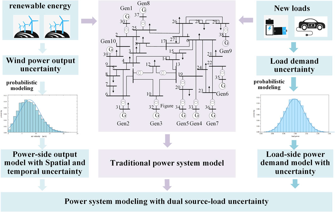
The increasing penetration of renewable energy sources into the power grid impacts its operational characteristics due to various factors, including weather, temperature, and other variables. As a result, the volatility of active power output intensifies, leading to heightened uncertainty in the power-side output of the system. Simultaneously, the grid load is progressively diversifying as numerous new loads, such as electric vehicles and distributed renewable energy sources. These new load types exhibit substantial power fluctuations, further exacerbating the uncertainty in power demand on the load side. The dual uncertainty on both the source and load sides works together to intensify the randomness of the operating conditions. After a power system failure, the power fluctuation resulting from source-load uncertainty and the power deficit caused by failure are superimposed on each other, thereby exacerbating the complexity of the incident, as illustrated in Figure 1.

Figure 1

Figure 1. Schematic diagram for uncertain source-load power modeling.

2.1 Wind power output model on power supply side considering spatial and temporal uncertainty

The uncertainty of wind power output is primarily influenced by wind speed. To more accurately simulate the actual variations in wind speed, it can be represented using probability distributions such as the Weibull distribution, Gaussian distribution, and Pearson distribution. Historical data indicates that the actual wind speed aligns most closely with the Weibull distribution’s probability density function. Therefore, this paper employs the Weibull distribution function to characterize the wind speed and establish a probabilistic representation of the uncertainty between the wind turbine’s output active power and wind speed. The wind speed probability density function of the Weibull distribution, denoted as f(v), and the cumulative distribution function of the Weibull distribution, denoted as F(v), as shown in Equations 1, 2:

$f\left(v\right)=\frac{K}{C}{\left(\frac{v}{C}\right)}^{K-1}\exp \left[-{\left(\frac{v}{C}\right)}^K\right](1)$

$F\left(v\right)=1-\exp \left[-{\left(\frac{v}{C}\right)}^K\right](2)$

Where v is the wind speed; K is the shape parameter of the Weibull distribution; C is the scale parameter of the Weibull distribution.

The characteristic curve of wind power output defines the relationship between wind power output and wind speed, where the intensity of wind speed directly influences the magnitude of the output. The relationship between wind power and wind speed can be described by a linear function, quadratic function, or cubic function, leading to distinct wind turbine power curves. Taking into account the actual statistical wind power data, wind power output is typically modeled using a cubic segmented function, which can be expressed as Equation 3:

$P_{\mathrm{W}}=\left\{\begin{array}{ll}0& v<v_{\text{in}}\text{or\hspace{0.5em}}v>v_{\text{out}}\\ P_{\mathrm{r}}\frac{v^3-v_{\text{in}}^3}{v_{\mathrm{r}}^3-v_{\text{in}}^3}& v_{\text{in}}\le v<v_{\mathrm{r}}\\ P_{\mathrm{r}}& v_{\mathrm{r}}\le v\le v_{\text{out}}\end{array}\right.(3)$

Where v_r, v_in, v_out are the rated wind speed, cut-in wind speed and cut-out wind speed of the wind farm turbine respectively; P_r is the rated power of the turbine.

Apart from temporal uncertainty, wind power output exhibits spatial correlation as well. Due to the close proximity of various wind farms within the same region and their placement in similar wind speed bands, a robust correlation exists between the outputs of different wind farms, consequently impacting the overall uncertainty of wind power. Hence, this section considers the spatial correlation among distinct wind farms and employs the Nataf inverse transformation principle to generate wind turbine output uncertainty data with predetermined correlation coefficients.

The theory of Nataf transform can transform random distribution variables with correlation into standard normal distribution variables that are independent of each other. The Nataf inverse transform serves as the reverse procedure to the Nataf transform, allowing the generation of distribution variables with desired correlation coefficients using independent standard normal distribution variables. This process facilitates the sampling of a significant amount of specified sample data.

Let the vector $P_{\mathrm{W}.i}\left(i=1,2,\dots ,n\right)$ represent the active outputs of n Weibull-distributed wind farms in the original correlation variable space. Similarly, let the vector $z_i\left(i=1,2,\dots ,n\right)$ denote the n standard normally distributed random variables in the correlation standard normal space. Subsequently, assume that the linear correlation coefficient matrices for Z and P_W are denoted by ρ₀ and ρ, respectively. Here, ρ is a predetermined value, and the relationship equation between the elements of the ρ₀ and ρ matrices is given as:

${\rho }_{0ij}=R_{ij}{\rho }_{ij}(4)$

$R_{ij}=1.063-0.004{\rho }_{ij}-0.200\left({\gamma }_i+{\gamma }_j\right)-0.001{\rho }_{ij}^2+0.337\left({\gamma }_i^2+{\gamma }_j^2\right)-0.007{\gamma }_i{\gamma }_j(5)$

Where γ_i and γ_j represent the computational parameters of the random variables P_i and P_j, respectively. The expressions for these parameters are given as follows Equation 6:

$\left\{\begin{array}{c}{\gamma }_i={\sigma }_i/{\mu }_i\\ {\gamma }_j={\sigma }_j/{\mu }_j\end{array}\right.(6)$

The positive definite symmetric matrix of correlation coefficients ρ₀ can be obtained through Equations 4, 5, and it can be decomposed into the lower triangular matrix B using the following expression Equation 7:

${\rho }_0=B{B}^{\mathrm{T}}(7)$

A standard normal distribution vector Z with specified correlation coefficients can be generated from the pre-obtained independent standard normal distribution vector X. The transformation is shown as Equation 8:

$Z=BX(8)$

Based on the equal probability transformation criterion, the standard normal distribution space with correlation is converted into correlated input vectors, i.e., wind power output variables that follow the Weibull distribution. The output power of each wind power node is given by Equation 9:

$P_{\mathrm{W}.i}=F_i^{-1}\left(\mathrm{\Phi }\left(z_i\right)\right)(9)$

Where P_{W. i} represents the correlated active power output of wind power node i; $F_i^{-1}\left(\cdot \right)$ is the inverse cumulative distribution function of the active power output of wind power node i; Φ(z_i) denotes the cumulative distribution function of z_i.

2.2 Load-side power demand modeling with uncertainties

The optimization strategy presented in this paper encompasses various novel controllable load types like electric vehicles, energy storage systems, commercial buildings, 5G base stations, and distributed photovoltaics. These loads can be directly enlisted by the emergency control system for urgent load shedding and contribute to the emergency frequency control of the power system. Unlike traditional methods that directly cut the load line during emergency frequency control, these controllable loads have a reduced impact on users when temporarily removed, resulting in lower load shedding costs. Furthermore, the power of these controllable loads can be precisely regulated by power electronic devices, enabling more flexible engagement in the power system’s emergency frequency control. The diverse characteristics of controllable loads introduce a complex influence on emergency frequency control, posing challenges in integrating them for considerations such as control continuity and data reliability. Consequently, the load side fluctuation range in modern power systems has expanded, while the time scale has diminished. This, in turn, has led to an escalation in power demand uncertainty, necessitating the characterization of load power uncertainty.

The probability of load power uncertainty is modeled using a normal distribution, which is expressed through a probability density function, as shown in Equation 10:

$\left\{\begin{array}{l}f\left(P_{\mathrm{L}}\right)=\frac{1}{\sqrt{2\mathrm{\pi }}{\sigma }_{P_{\mathrm{L}}}}\exp \left(-\frac{{\left(P_{\mathrm{L}}-{\mu }_{P_{\mathrm{L}}}\right)}^2}{2{\sigma }_{P_{\mathrm{L}}}^2}\right)\\ f\left(Q_{\mathrm{L}}\right)=\frac{1}{\sqrt{2\mathrm{\pi }}{\sigma }_{Q_{\mathrm{L}}}}\exp \left(-\frac{{\left(Q_{\mathrm{L}}-{\mu }_{Q_{\mathrm{L}}}\right)}^2}{2{\sigma }_{Q_{\mathrm{L}}}^2}\right)\end{array}\right.(10)$

Where P_L and Q_L represent the active and reactive power of the load, respectively; μ_PL and μ_QL denote the expected values of the active and reactive power of the load, respectively; σ_PL and σ_QL indicate the standard deviation of the active and reactive power of the load, respectively.

Additionally, the presence of various new controllable loads on the load side, such as electric vehicles and energy storage, introduces variability and diversity in load characteristics. The complexity of these controllable load components further contributes to the uncertainty of overall load characteristics. Determining the controllable load characteristics directly becomes infeasible when the power system’s operating state changes, necessitating the expression of uncertainty through a probability distribution. Consequently, a novel static load model should be established utilizing frequency and voltage indices that adhere to the probability distribution, as Equation 11.

$\begin{array}{l}{P}_{\mathrm{L}.\text{new}}^{\prime }=P_{\mathrm{L}}{\left(U/U_{\mathrm{N}}\right)}^{{k_{pu}}_{.\text{new}}}\left(1+{k_{pf}}_{.\text{new}}\left(f-f_{\mathrm{N}}\right)\right)\\ Q_{\mathrm{L}.\text{new}}^{\prime }=Q_{\mathrm{L}}{\left(U/U_{\mathrm{N}}\right)}^{{k_{qu}}_{.\text{new}}}\left(1+{k_{qf}}_{.\text{new}}\left(f-f_{\mathrm{N}}\right)\right)\end{array}(11)$

Where k_{pu. new} and k_{qu. new} represent voltage indices of active and reactive power of the new controllable loads, respectively; k_{pf. new} and k_{qf. new} denote frequency indices of active and reactive power of the loads, respectively.

These parameters, k_{pu. new}, k_{qu. new}, k_{pf. new} and k_{qf. new}, are subject to uncertainty and are characterized by probability distributions that follow a normal distribution.

In summary, considering the uncertainty of load size, which is represented by P_L and Q_L that conform to normal distribution, and considering the uncertainty of load characteristics, which is represented by P^’_L.new and Q^’_L.new that contain time-varying load coefficients, a power demand uncertainty model that integrally considers fluctuations in load quantity and fluctuations in load characteristics is thus established.

3 Improvement of the MDP model for emergency frequency control problem in source-load dual uncertainty power system

Reinforcement learning can be formulated through MDP, which performs policy search through the set (S, A, P, R, y). Where S is the state space and A is the action space, which can be either continuous or discrete. P is the state transfer probability, which represents the probability density of the next state s_t+1 given the current state s_t ∈ S and the current action a_t∈A. R is the reward function and y is the discount factor. Most of the classical MDP theories and RL algorithms are based on discrete-time leapfrog actions, but many power system control problems follow continuous-time dynamics actions, which can only be discretized by using appropriate time intervals to cut the continuous-time dynamics. Therefore, this paper addresses this drawback by using an MDP model for improving the emergency frequency control of the system and optimizing the emergency frequency control strategy using the deep reinforcement learning SAC algorithm with continuous action space.

3.1 State space

Power system emergency frequency stabilization is closely related to generator active power, load power, system frequency, and the rate of frequency change. Considering the dual source-load uncertainty in power-side active output and demand-side active load, it is necessary to incorporate all generator active output and load node power with uncertainty into the state space, defining the state space s_t as Equation 12:

$\begin{array}{l}{s}_t=s_1^t\cup s_2^t\cup s_3^t\cup s_4^t\\ \left\{\begin{array}{l}{s}_1^t=\left\{\begin{array}{cccc}{f}_1^t& f_2^t& \cdots & f_m^t\end{array}\right\}\\ s_2^t=\left\{\begin{array}{cccc}{\left(\mathrm{d}f/\mathrm{d}t\right)}_1^t& {\left(\mathrm{d}f/\mathrm{d}t\right)}_2^t& \cdots & {\left(\mathrm{d}f/\mathrm{d}t\right)}_m^t\end{array}\right\}\\ s_3^t=\left\{\begin{array}{cccc}{P}_{\mathrm{e}.1}^t& P_{\mathrm{e}.2}^t& \cdots & P_{\mathrm{e}.m}^t\end{array}\right\}\\ s_4^t=\left\{\begin{array}{cccc}{P}_{\mathrm{l}.1}^t& P_{\mathrm{l}.2}^t& \cdots & P_{\mathrm{l}.n}^t\end{array}\right\}\end{array}\right.\end{array}(12)$

Where f_i^t is the frequency of generator node i at moment t; (df/dt)_i^t is the frequency change rate of generator node i at moment t; P_{e. i}^t is the electromagnetic power of generator node i at moment t; P_{l. j}^t is the active load of load node j at moment t.

3.2 Action space

The control action of each controllable load at moment t should be to reduce a part of the total controllable load at that node. Due to the uncertainty of load demand power, the total controllable load needs to be updated in real time. However, for uniformity of the control action, the action space must be fixed. Therefore, the action space is set as the proportion of the controllable load removed at each node. The actual load reduction is the value of the action at each node multiplied by the total controllable load at that node. Consequently, each controllable load action is defined as a continuous value within [-1, 0], and the total action space is shown as Equation 13:

$a_t=\left\{\begin{array}{cccc}\Delta P_1^t& \Delta P_2^t& \cdots & \Delta P_n^t\end{array}\right\}(13)$

Where ΔP_m^t is the load removal of controllable load node m at time t and ΔP_m^t∈[−1,0]; n is the number of controllable load nodes.

3.3 Reward functions

The goal of the emergency frequency control problem is to restore the frequency to within the stabilization range quickly while minimizing load shedding. For source-load dual uncertainty power systems, the effectiveness of emergency frequency control is primarily evaluated in terms of frequency deviation and load shedding amount.

Therefore, the reward function consists of three parts: 1) the average value of steady-state frequency deviation over a specific time period at the end of the simulation; 2) a penalty term calculated based on controllable load importance and load shedding; and 3) a penalty term for exceeding the lowest point of the system’s dynamic frequency. The expression is shown as Equation 14:

$\begin{array}{l}{r}_t={\lambda }_1\left|\Delta f_{T_{\text{tem}}}\right|-{\lambda }_2{\displaystyle \sum _{j=1}^n}{C}_j{P}_{\text{sl}.j}-H_1\\ H_1=\left\{\begin{array}{ll}-100,& \text{if\hspace{0.17em}}\left(f_{\min }<f_{\min .\text{set}}\right)\\ 0,& \text{therwise}\end{array}\right.\end{array}(14)$

Where T_tem is a certain time period before the end of the simulation process; Δf_Ttem is the average value of the deviation of the center of frequency inertia during T_tem; C_j is the importance index of load node j; P_{sl. j} is the amount of load shedding at node j; H₁ is the penalty for the system’s center of frequency inertia when the minimum value is less than the integrating value; λ₁ and λ₂ are coefficients for each part of the reward function.

4 Optimization of emergency frequency control strategy considering dual source-load uncertainties

Emergency frequency control is a kind of multi-constraint multi-objective optimization problem, which needs to consider two conflicting objectives of fast frequency recovery and minimizing control cost at the same time. Moreover, it often exhibits a propensity to favor one objective over the other, leading to convergence on local optimal solutions. The SAC algorithm introduces the action entropy value to balance the probability of the various action strategies in the action space, to avoid learning the same action repeatedly and falling into the sub-optimal solution, and it has a stronger exploratory ability, and is more suitable for the studying the emergency frequency control problem with multiple objectives.

Following a failure in a power system that considers dual source-load uncertainty, the power deficit resulting from the disturbance combines with the source-load uncertainty, resulting in increased random volatility in the collected grid state data and causing ongoing oscillations in the training process. Faced with this high level of uncertainty, some DRL algorithms based on strategy gradient exhibit weak generalization abilities, leading to unstable emergency frequency control effects. In contrast, the SAC algorithm incorporates action entropy, enhancing robustness and resistance to disturbances, and demonstrating stronger learning generalization capabilities, rendering it more suitable for the dual source-load uncertainty power system discussed in this chapter.

Moreover, the SAC algorithm features a continuous action space, eliminating the need for discretizing load removal actions. This allows for the removal of the required load amount at once, thereby preventing exacerbation of frequency drop depth resulting from multiple actions. Additionally, continuous action space control enhances precision and reduces the likelihood of excessive or inadequate load removal during emergency frequency control. This ensures a smaller steady-state frequency deviation post-control while minimizing the amount of load removed.

The SAC algorithm offers higher exploration capability, improved robustness, and a continuous action space compared to other DRL algorithms. Consequently, the SAC algorithm is employed in this section to optimize the emergency frequency control strategy for source-load dual uncertainty power systems.

4.1 Principle of SAC algorithm and network structure

The SAC algorithm belongs to the deep reinforcement learning algorithms based on the value function, which incorporates a mechanism that encourages exploration through action strategy entropy values. This enhances the algorithm’s robustness compared to other strategy gradient-based DRL algorithms like PPO, A3C, and DDPG. The entropy value, defined as the expectation of information quantity, quantifies the uncertainty of a variable. It increases with the uncertainty of an event and can be quantified by the event’s probability. The entropy value is defined as Equation 15:

$H\left(X\right)=-{\displaystyle \sum _{x_i\in X}}l\left(x_i\right)\ln l\left(x_i\right)(15)$

Where H(X) is the entropy value; l (x_i) is the event probability.

The DRL algorithm should continuously explore the interaction environment to accumulate experience and avoid selecting too many actions solely based on immediate rewards, as this may lead to convergence on local optimal solutions. The SAC algorithm considers the maximum entropy value of actions. If the entropy value decreases due to repeated selection of a certain action, the maximum entropy mechanism encourages the agent to explore other actions, thus broadening the exploration range and increasing the algorithm’s robustness.

In other deep reinforcement learning algorithms with stochastic policies, the objective of model learning is clear: to derive an optimal action policy that maximizes the expected cumulative reward through straightforward training. The optimal policy expression is shown as Equation 16:

$\pi ={\mathrm{argmax}}_{\pi }{E}_{\left(s_t,a_t\right)\sim {\rho }_{\pi }}\left[{\displaystyle \sum _t}r\left(s_t,a_t\right)\right](16)$

The SAC algorithm necessitates maximizing the entropy value of the output action to enhance exploration capability. In other words, an additional term regarding the entropy value is incorporated into the policy expression, resulting in the expression of the improved optimal policy as shown in Equation 17:

$\pi ={\mathrm{argmax}}_{\pi }{E}_{\left(s_t,a_t\right)\sim P_{\pi }}\left[{\displaystyle \sum _t}\underset{\text{reward}}{\underbrace{r\left(s_t,a_t\right)}}+\alpha \underset{\text{entropy}}{\underbrace{H\left(\pi \left(\cdot \mid s_t\right)\right)}}\right](17)$

Where E (s_t, a_t) denotes the expectation function; π represents the strategy; s_t and a_t signify the state space and action space at moment t; r (s_t, a_t) denotes the reward function at moment t (s_t, a_t)∼P_π signifies the trajectory of state-action under strategy π; + is the automatic entropy temperature parameter, which adjusts the entropy value affecting the degree of rewards; and H (π(⋅|s_t)) signifies the entropy of the output action of the strategyπ under the state s_t, as expressed below in Equation 18:

$\begin{array}{l}H\left(\pi \left(\cdot \mid s_t\right)\right)=-\sum \pi \left(\cdot \mid s_t\right)\log \left(\pi \left(\cdot \mid s_t\right)\right)\\ =-\underset{a_t}{\int }P\left(\pi \left(a_t\mid s_t\right)\right)\ln P\left(\pi \left(a_t\mid s_t\right)\right)\mathrm{d}{a}_t\end{array}(18)$

Where P (π (a_t|s_t)) denotes the probability that the action value at the time of t is a_t.

In the SAC algorithm for strategy value evaluation, the expression for updating the strategy using the Bellman operator is expressed as Equation 19:

$Q^{\pi }\left(s_t,a_t\right)=r_t+E\left[{\displaystyle \sum _{t=1}^{\infty }}{\gamma }^t\left[r\left(s_t,a_t\right)-\alpha \log \pi \left(a_t\mid s_t\right)\right]\right](19)$

Where γ denotes the discount factor at the time of strategy update.

The optimal policy can be continuously learned and refined through policy iteration, comprising two steps: soft policy evaluation and soft policy improvement. Firstly, in the strategy evaluation step, the soft value update function of a given strategy π can be obtained using the soft Bellman operator, as shown in Equation 20:

${\mathcal{T}}^{\pi }{Q}^{\pi }\left(s,a\right)=r+\gamma E_{s^{\prime }}\left[Q^{\pi }\left(s^{\prime },a^{\prime }\right)-\alpha \log \pi \left(a^{\prime }\mid s^{\prime }\right)\right](20)$

The SAC algorithm belongs to the Actor-Critic class of algorithms, where the Actor is employed for policy modeling and the Critic for Q-value function modeling. Different deep neural networks are utilized to fit the Q-value function and the policy function, respectively, as shown in Equation 21:

$J_Q\left(\theta \right)=E\left[\frac{1}{2}(Q\left(s_t,a_t\right)-{\left(r\left(s_t,a_t\right)+\gamma V_{\overline{\theta }}\left(s_{t+1}\right)\right)}^2\right](21)$

Where θ denotes the parameters of the policy network; $V_{\overline{\theta }}$ represents the updated value function value.

Both networks are optimized using independent gradients ${\widehat{\nabla }}_{\theta }{J}_Q\left(\theta \right)$ , as expressed in Equation 22:

${\widehat{\nabla }}_{\theta }{J}_Q\left(\theta \right)={\nabla }_{\theta }{Q}_{\theta }\left(s_t,a_t\right)\cdot \left(\Delta Q_{\theta }\right)(22)$

Where the expression of ΔQ_θ is expressed as Equation 23:

$\begin{array}{l}\Delta Q_{\theta }=Q_{\theta }\left(s_t,a_t\right)-r\left(s_t,a_t\right)\\ +\gamma \left(Q_{\overline{\theta }}\left(s_{t+1},a_{t+1}\right)-\alpha \log \left({\pi }_{\varphi }\left(a_{t+1}\mid s_{t+1}\right)\right)\right)\end{array}(23)$

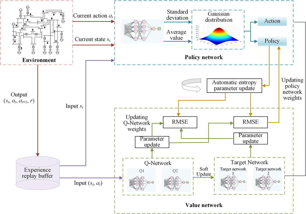
The outputs of the policy network are the mean and standard deviation values following a Gaussian distribution. The network with the smaller Q value is selected to reduce bias in updating the parameters of the policy network. The approximate gradient of the parameter update is expressed as Equation 24:

$\begin{array}{l}{\widehat{\nabla }}_{\varphi }{J}_{\pi }\left(\varphi \right)={\nabla }_{\varphi }\alpha \log \left({\pi }_{\varphi }\left(a_t\mid s_t\right)\right)\\ +\left({\nabla }_{a_t}\alpha \log \left({\pi }_{\varphi }\left(a_t\mid s_t\right)\right)-{\nabla }_{a_t}Q\left(s_t,a_t\right)\right){\nabla }_{\varphi }{f}_{\varphi }\left({\epsilon }_t;s_t\right)\end{array}(24)$

At the same time, the action entropy value is also updated in the policy network, making it crucial to choose the appropriate temperature parameter, α. As the reward value varies during the training process, fixing the temperature coefficient reduces the stability of model training. Therefore, the temperature coefficient α is generally updated automatically by minimizing J (α), as expressed in Equation 25:

$J\left(\alpha \right)=E_{a_t-{\pi }_i}\left[-\alpha \log \left({\pi }_t\left(a_t\mid s_t\right)\right)-\alpha M\right](25)$

Where M represents the dimension of the action matrix, specifically denoted as M = dim(a).

The SAC algorithm for deep reinforcement learning comprises four crucial components: the experience replay buffer, the automatic entropy parameter, the policy network, and the value network. The experience replay buffer stores historical exploration experience, while the automatic entropy parameter stabilizes and adjusts the exploration strategy. The policy network is responsible for action selection, and the value network estimates state-action values. The overall structure of the algorithm is depicted in Figure 2.

Figure 2

Figure 2. Structure of SAC algorithm.

4.2 Optimization of emergency frequency control strategy based on SAC algorithm

When utilizing the SAC algorithm to optimize the emergency frequency control strategy, each iterative training process can be summarized into three main steps: firstly, collecting and inputting the operating state data of the power system after the fault into the SAC model; then, the SAC model selects the emergency frequency control action based on the state data; finally, executing the control action on the power system simulation environment to achieve the objective. Additionally, due to the uncertain nature of source-load power systems, it is necessary to incorporate an uncertainty model for wind power output and load demand in each interaction process. The overall process of emergency frequency control for a source-load dual uncertainty system based on the SAC algorithm is illustrated in Figure 3.

Figure 3

Figure 3. Flow chart of emergency frequency control based on SAC algorithm.

Prior to model training, the simulation environment and SAC model parameters are initialized. The power system load factor is randomly initialized, and the model incorporates uncertainty in wind power output and load demand. The Nataf inversion theory is employed to generate source-load dual uncertainty power samples with correlation. Before each interactive training step, uncertainty power samples are randomly assigned to wind turbine nodes, and uncertainty load demand samples are added to load nodes to simulate real-world source-load uncertainty power system conditions. Subsequently, the SAC model obtains the current system state data from the simulation environment, selects an action based on an environmental state update policy, and delivers it to the simulation environment. After receiving the emergency frequency control action from the SAC model, the simulated power system environment executes the load adjustment action, advances to the next state, and sends the updated state data and immediate reward value to the SAC model. This training process continues until the end of a round, marked by maintaining stable system frequency. At this point, the system simulation environment is reinitialized, and the next round begins. Upon completing the training process, the SAC model can be applied to various fault test scenarios to validate its effectiveness and superiority.

5 Simulation analysis

To evaluate the effectiveness of the proposed method in this paper, a deep reinforcement learning environment is constructed to enhance the IEEE10 machine with 39 nodes. This environment is developed using Python and BPA simulation software. The SAC algorithm is employed to solve the specified test cases. The deep neural network is implemented in Python using TensorFlow 1.15. The experiments are conducted on an Intel Core i5-11400H CPU with 16.00 GB RAM and an RTX 3050 GPU.

5.1 Data of the test case

The BPA software is utilized in this paper to generate a fault scenario for the IEEE10 machine with 39 nodes. The generator model is based on the sixth order model, while the load model consists of a constant impedance model and a mixed load model incorporating induction motors, with a 50% ratio between the two. The fault scenario involves a generator experiencing a partial power loss, resulting in a power difference within the power system. The total simulation time is 40 s, with each cycle of the waveform serving as a sampling point. To simulate various system fault states and obtain sufficient samples, one of the ten generators is randomly selected at the start of the simulation to experience a loss of active output ranging from 0.5 p. u. to one p. u.

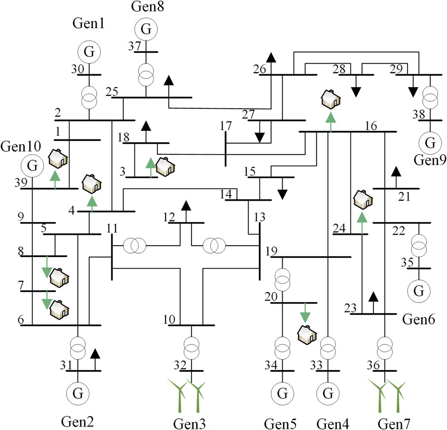
This paper utilizes a modified version of the IEEE10 machine with 39 nodes to validate the proposed methodology in this section. The modification involves replacing nodes 32 and 36 with turbines having rated capacities of 684 MW and 576 MW, respectively. Additionally, nodes 3, 4, 7, 8, 16, 20, 24, and 39 are designated as controllable load nodes participating in frequency emergency control. The system’s topology is illustrated in Figure 4.

Figure 4

Figure 4. Improved topology of IEEE39 nodes.

The power fluctuations at the load nodes follow a normal distribution with a mean and standard deviation equal to 5% of the rated value. Similarly, the load static model voltage and frequency indices also have a mean and standard deviation of 5% of the rated value.

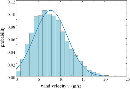
The wind speeds of the wind nodes are modeled by a Weibull distribution with the shape parameter K set to 2.26, the scale parameter C set to 7.55, the cut-in wind speed at 3.5 m/s, the cut-out wind speed at 25 m/s, and the rated wind speed at 7.3 m/s.

To account for the correlation between the wind turbine nodes, 1,000 sets of wind turbine output samples are generated using the Nataf inverse transformations, with correlation coefficients of 0.8. Figure 5 illustrates the Weibull distribution of wind speed.

Figure 5

Figure 5. Weibull distribution of wind speed.

The deep reinforcement learning state space in this system comprises frequency deviation, frequency rate of change, active output, and load of each node, resulting in a 47-dimensional space. The action space consists of eight load shedding actions for controllable loads. Each action is represented as an 8-dimensional vector, where each element is a continuous value within the range of [-1, 0]. Furthermore, as the Soft Actor Critic (SAC) algorithm can handle continuous action spaces, the emergency frequency control directly determines the necessary load shedding amount and sets the action time for emergency frequency control as 2 s after fault detection. The delay characteristics of controllable loads are categorized into three levels. For loads of the same delay level, the actual control delay is calculated based on the maximum value to ensure that the actual frequency drop depth is less than or equal to the ideal frequency drop depth, thereby avoiding frequency instability. Consequently, after aggregation, it is assumed that the control delay for all level 1 controllable loads is 100 ms, for level 2 controllable loads is 200 ms, and for level 3 controllable loads is 300 ms. The controllable loads are then removed within each node in order of delay from low to high. Table 1 provides the proportions of controllable loads at each node and the distribution of loads across different control delay levels after aggregated modeling.

Table 1

Table 1. The proportion of load with different time delay levels.

5.2 Analysis of model training and testing results

The policy network and value network of the SAC model both consist of two hidden layers with 64 neurons each. The activation function is set to ReLU, the learning rate is 0.005, the initial temperature coefficient is 0.1, the self-updating learning rate is 0.0001, and the updating algorithms utilize the alternating multiplier method. The experience replay unit has a capacity of 2,500, and 64 samples are drawn for each training iteration. The convergence criterion for each training round is that the absolute value of the steady-state frequency deviation is less than 0.1 Hz.

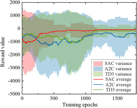
The SAC algorithm is employed to learn and train the aforementioned arithmetic model. Figure 6 depict the curves illustrating the changes in reward values during the training process.

Figure 6

Figure 6. Changes in reward values during training.

Figure 6 demonstrate that, initially, the model struggles to find a control strategy that effectively stabilizes the system frequency, resulting in frequent movements per round and consequently low reward values. Additionally, the maximum number of action steps per round often reaches 50. However, as training progresses, the model gradually discovers more efficient control strategies with shorter action sequences, although the reward value remains suboptimal due to excessive load removal. It is only after 1,200 rounds of training that both the reward value and the number of training rounds stabilize, indicating the completion of the model training process.

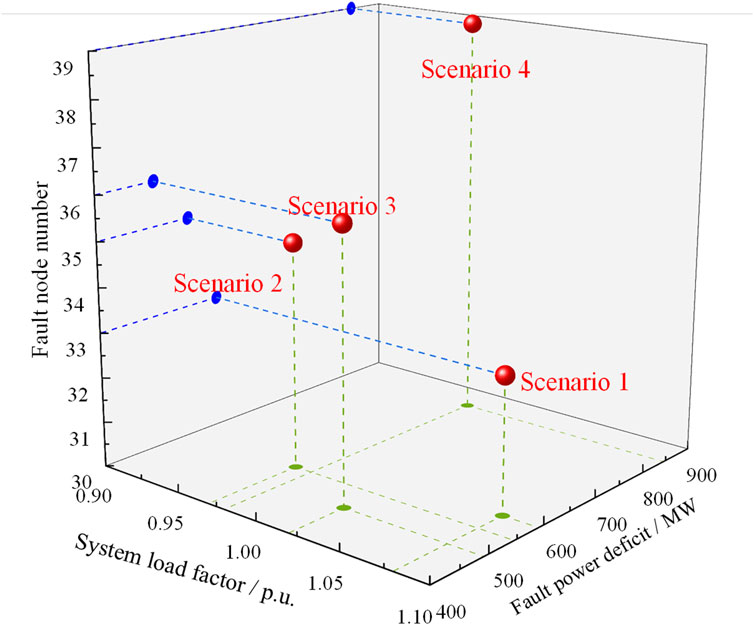
To evaluate and compare the frequency recovery process of the proposed emergency frequency control scheme, it is essential to conduct tests using various fault scenarios. These scenarios are characterized by four attributes: the number of faulty nodes, the extent of power shortage in the faulty nodes, the system load factor, and the magnitude of source load fluctuations. For this purpose, four representative fault scenarios are selected, as illustrated in Figure 7.

Figure 7

Figure 7. Number of excision maneuvers during each training round.

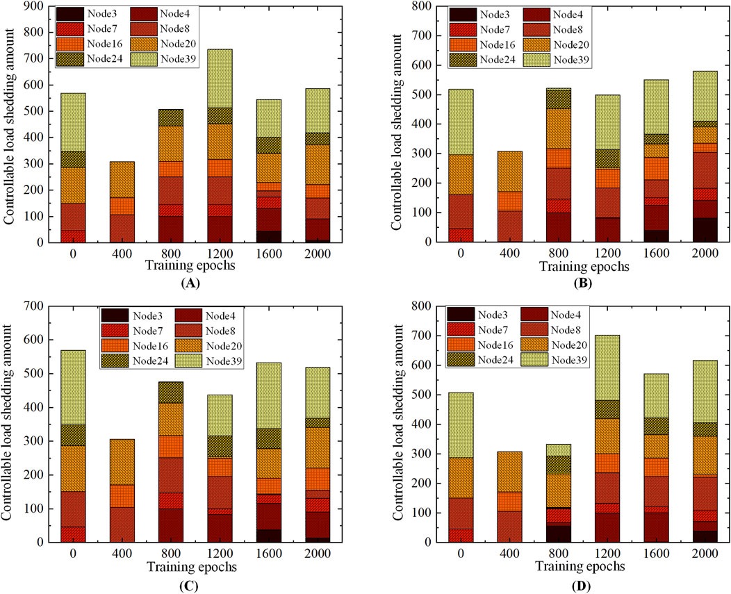
During the model training process, the emergency frequency control policies for the four representative scenarios are derived through testing at intervals of 400 rounds until the completion of 2000 rounds, leading to the acquisition of the optimal control policy, as depicted in Figure 8.

Figure 8

Figure 8. Change process of load shedding strategy in scenario (A–D) training.

Figure 8 clearly demonstrate significant fluctuations in the emergency frequency control strategies during rounds 0, 400, 800, and 1,200, indicating the model’s continuous search for an improved control strategy. In contrast, the control strategies for rounds 1,600 and 2000 exhibit reduced fluctuations, indicating that the model has undergone substantial training. Initially, the emergency frequency control strategy is more random, but through continuous training, the model takes into account factors such as the amount of controllable loads at each node and load removal sensitivity. Consequently, it selects an optimal node for load shedding, resulting in a final strategy with total load removal close to the power deficit.

Table 2 presents the controllable load shedding quantities for the optimal policy in the four representative test scenarios, along with the steady-state frequency values achieved post-policy implementation and the minimum value of dynamic frequency drop.

Table 2

Table 2. Controllable load shedding and dynamic frequency metrics for various test scenarios.

Table 2 reveals that in the four test scenarios, characterized by diverse fault locations, fault sizes, system loading rates, and source-load uncertainties, the trained model successfully maintains the system within 0.1 Hz of the steady-state frequency deviation. Additionally, the lowest point of the dynamic frequency drop remains above 49.5 Hz. These results substantiate the effectiveness of the emergency control strategy based on the SAC algorithm, particularly for systems affected by source-load uncertainties.

To further ascertain the superiority of the proposed method, a comparative analysis is conducted between the emergency frequency control strategy derived from the traditional adaptive UFLS algorithm and the strategy proposed in this paper. The dynamic frequency recovery process of the system is evaluated for both strategies across the four scenarios, as depicted in Figure 9.

Figure 9

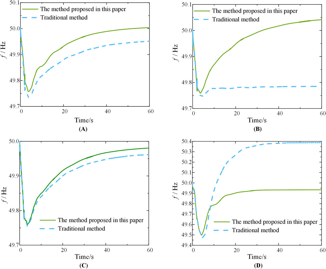
Figure 9. Comparison of the dynamic frequency process of scenario (A–D) after the execution of the two strategies.

Figure 9 demonstrates that the emergency frequency control strategies optimized by the proposed scheme in this paper effectively maintain the steady-state frequency deviation of the system within 0.1 Hz, with the lowest frequency point exceeding 49.5 Hz across the four different scenarios. In contrast, the adaptive UFLS scheme in Scenarios 1, 2, and three suffers from the issue of insufficient load shedding, resulting in a greater depth of frequency drop and steady-state frequency deviation. Additionally, the conventional scheme in Scenario four exhibits excessive load shedding, leading to a steady-state frequency close to 50.4 Hz. Consequently, the method presented in this chapter proves its superiority in reducing the depth of frequency drop and steady-state frequency deviation, highlighting the effectiveness of the deep reinforcement learning algorithm.

To compare the disparities between source-load uncertainty and deterministic power systems, both the conventional method and the SAC algorithm proposed in this chapter are employed in both systems for 100 tests. The emergency frequency control outcomes are then compared, and the results are illustrated in Figure 10.

Figure 10

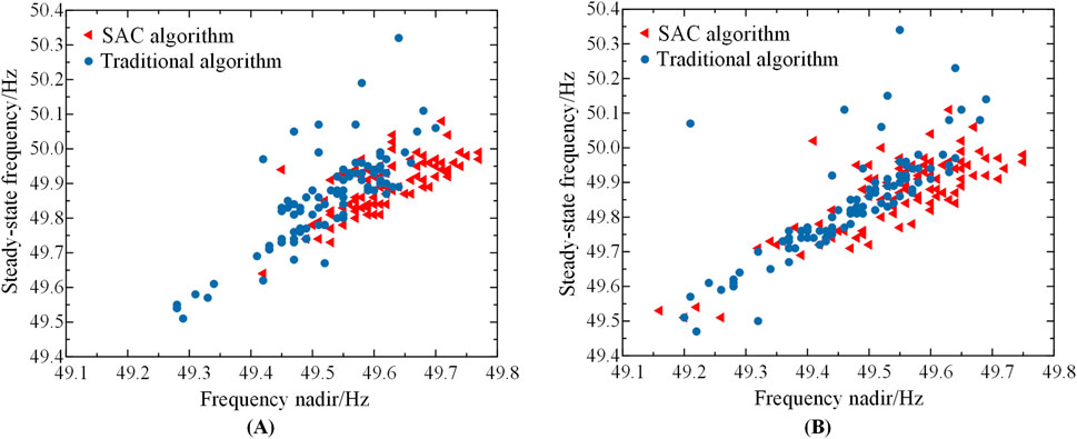
Figure 10. (A) Comparison of stochastic test results for source-load deterministic systems (B). Comparison of stochastic test results for the source-load uncertainty system.

Figures 10A, B reveal that the median frequency nadir achieved by the SAC algorithm in the source-load deterministic system and the uncertain system is approximately 49.65 Hz and 49.6 Hz, respectively, whereas the median values obtained by the traditional method are around 49.55 Hz and 49.45 Hz, respectively. Notably, the frequency nadir resulting from the traditional method is significantly lower than that achieved by the deep reinforcement learning method, making it nearly impossible to maintain system frequency stability in numerous scenarios. By contrast, the SAC algorithm effectively improves the steady-state frequency deviation and frequency nadir in both deterministic and uncertain systems, demonstrating its superiority over the traditional method for addressing the emergency frequency control problem in source-load uncertain systems.

To validate the suitability of the SAC algorithm over other reinforcement learning algorithms for addressing the emergency frequency control problem in the source-load double uncertainty system, the model developed based on the SAC algorithm in this paper is compared with models employing the A2C algorithm and the TD3 algorithm. Figure 11 presents a comparison of the reward value’s increasing trend throughout the training process. The solid line represents the smoothed reward value, while the shaded area denotes the variance fluctuation of the reward value.

Figure 11

Figure 11. Comparison of reward values of different DRL algorithms.

Figure 11 illustrates that after approximately 500 rounds, the smoothed reward value of the model based on the SAC algorithm surpasses that of the other algorithm models, exhibiting a gradual increase until it stabilizes at the desired value. Furthermore, in terms of variance, the reward value’s variance for the SAC algorithm is higher during the initial 300 training rounds and subsequently becomes smaller than that of the other two algorithms. This observation indicates the robustness of the SAC algorithm, its ability to swiftly enhance the reward value through learning, and its reduced oscillation.

The SAC algorithm effectively decreases the minimum system frequency drop compared to other DRL algorithms, while also reducing the steady-state frequency deviation. To visually demonstrate the test’s improvement more intuitively, Figure 12A and (B) present the distribution of frequency drop nadir and steady-state frequency deviations resulting from the tests conducted with various algorithms under random scenarios.

Figure 12

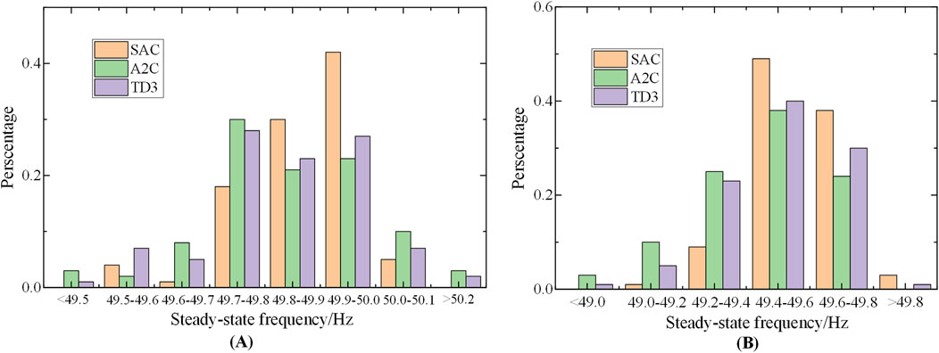
Figure 12. (A) Comparison of steady-state frequency deviation distribution of different DRL algorithms for random testing (B). Comparison of frequency drop nadir distribution of different DRL algorithms for random testing.

As can be seen from Figure 12, the test results of the emergency frequency control strategy using the SAC algorithm show that the probability of the system’s steady-state frequency stabilizing at 49.8Hz–50 Hz is more than 50%, which is much higher than that of the test results using the A2C and TD3 algorithms, and the probability of the frequency dip nadir of the SAC algorithm being higher than 49.4 Hz is much higher than that of the other two algorithms. Therefore, the model based on SAC algorithm in this chapter can effectively improve the dynamic frequency nadir and steady-state frequency of the system after emergency frequency control compared to other DRL algorithms.

6 Conclusion

The emerging power systems exhibit dual source-load uncertainty, contributing to the increasing nonlinearity and complexity of the emergency frequency stabilization problem. Consequently, this paper proposes an optimization method based on the SAC algorithm for the emergency frequency control strategy of power systems with dual source-load uncertainty. Experimental verification is conducted through the design of various operational scenarios, yielding the following conclusions.

1) The dual uncertainty in the new power system, stemming from both source and load, is analyzed. This includes the spatio-temporal uncertainty of wind power output on the power source side and the uncertainty in power demand on the load side. This analysis aims to prevent errors caused by the superposition of uncertain power from both sources and the fault power deficit.

2) Enhance the state space, action space, and reward function of the emergency frequency control MDP model to accommodate the characteristics of source-load double uncertainty;

3) Finally, the proposed method is validated in a modified IEEE10 machine 39-node system incorporating source-load uncertainty. The results demonstrate that the proposed model accounts for the superposition of source-load uncertainty power and fault power, leading to a reduction in steady-state frequency deviation after emergency frequency control. Moreover, compared with the traditional UFLS method and other DRL algorithms, the SAC algorithm with continuous action space accurately removes the load in a single pass, thereby enhancing the frequency restoration speed and minimizing the cost of controllable load removal.

Data availability statement

The raw data supporting the conclusions of this article will be made available by the authors, without undue reservation.

Author contributions

SZ: Conceptualization, Funding acquisition, Writing–original draft, Writing–review and editing. SR: Project administration, Writing–review and editing. BZ: Formal Analysis, Writing–review and editing. JF: Validation, Writing–original draft, Supervision. XZ: Validation, Writing–review and editing. YW: Writing–original draft, Writing–review and editing, Supervision. LS: Funding acquisition, Writing–original draft, Writing–review and editing, Methodology, Software.

Funding

The author(s) declare that financial support was received for the research, authorship, and/or publication of this article. This work was supported by the National Natural Science Foundation of China (52077059).

Conflict of interest

Authors SZ, SR, BZ, JF, XZ was employed by Longyuan(Beijing)Wind Power Engineering Technology Co., Ltd. Author YW was employed by State Grid Jiangsu Electric Power Co., Ltd.

The remaining author declares that the research was conducted in the absence of any commercial or financial relationships that could be construed as a potential conflict of interest.

Publisher’s note

All claims expressed in this article are solely those of the authors and do not necessarily represent those of their affiliated organizations, or those of the publisher, the editors and the reviewers. Any product that may be evaluated in this article, or claim that may be made by its manufacturer, is not guaranteed or endorsed by the publisher.

References

Bai, F., Wang, X., Liu, Y., Liu, X., Xiang, Y., and Liu, Y. (2016). Measurement-based frequency dynamic response estimation using geometric template matching and recurrent artificial neural network. CSEE J. Power Energy Syst. 2, 10–18. doi:10.17775/cseejpes.2016.00030JPES.2016.00030

CrossRef Full Text | Google Scholar

Cao, Y., Zhang, H., Zhang, Y., and Li, C. (2021). Event-driven fast frequency response control method for generator unit. Automation Electr. Power Syst. 45, 148–154. doi:10.7500/AEPS20210210001

CrossRef Full Text | Google Scholar

Chandra, A., and Pradhan, A. K. (2020). An adaptive underfrequency load shedding scheme in the presence of solar photovoltaic plants. IEEE Syst. J., 1–10.

Google Scholar

Chen, C., Cui, M., Li, F., Yin, S., and Wang, X. (2020). Model-free emergency frequency control based on reinforcement learning. IEEE Trans. Industrial Inf. 17, 2336–2346. doi:10.1109/tii.2020.3001095

CrossRef Full Text | Google Scholar

Dai, Y., Xu, Y., Dong, Z. Y., Wong, K. P., and Zhuang, L. (2012). Real-time prediction of event-driven load shedding for frequency stability enhancement of power systems. IET Generation, Transm. and Distribution. 6, 914–921. doi:10.1049/iet-gtd.2011.0810

CrossRef Full Text | Google Scholar

Hu, Yi, Wang, X., Teng, Y., Ai, P., and Che, Y. (2019). Frequency stability control method of AC/DC power system based on multi-layer support vector machine. Proc. CSEE 39, 4104–4118. doi:10.13334/j.0258-8013.pcsee.181496

CrossRef Full Text | Google Scholar

Ke, D., Feng, S., Liu, F., Chang, H., and Sun, Y. (2022). Rapid optimization for emergent frequency control strategy with the power regulation of renewable energy during the loss of DC connection. Trans. China Electrotech. Soc. 37, 1204–1218. doi:10.19595/j.cnki.1000-6753.tces.210279

CrossRef Full Text | Google Scholar

Larik, R. M., Mustafa, M. W., Aman, M. N., Jumani, T. A., Sajid, S., and Panjwani, M. K. (2018). An improved algorithm for optimal load shedding in power systems. Energies 11, 1808. doi:10.3390/en11071808

CrossRef Full Text | Google Scholar

Li, C., Wu, Y., Sun, Y., Zhang, H., Liu, Y., Liu, Y., et al. (2020). Continuous under-frequency load shedding scheme for power system adaptive frequency control. IEEE Trans. Power Syst. 35, 950–961. doi:10.1109/TPWRS.2019.2943150

CrossRef Full Text | Google Scholar

Li, S., Liao, Q., Tang, F., Zhao, H., and Shao, Y. (2017). Adaptive underfrequency load shedding strategy considering high wind power penetration. Power Syst. Technol. 41, 1084Y1090. doi:10.13335/j.1000-3673.pst.2016.3029

CrossRef Full Text | Google Scholar

Lin, H. (2022). Transient stability analysis and control of AC-DC hybrid power grid under topology changes based on deep learning. Beijing, China: North China Electric Power University.

Google Scholar

Liu, K., Wang, X., and Bo, Q. (2014). Minimum frequency prediction of power system after disturbance based on the WAMS data. Proc. CSEE 34, 2188–2195. doi:10.13334/j.0258-8013.pcsee.2014.13.021

CrossRef Full Text | Google Scholar

Ma, Q., Zhang, H., He, X., Tang, J., Yuan, X., and Wang, G. (2020). “Emergency frequency control strategy using demand response based on deep reinforcement learning,” in 2020 12th IEEE PES asia-pacific power and energy engineering conference (Nanjing, China: APPEEC), 1–5. doi:10.1109/APPEEC48164.2020.9220600

CrossRef Full Text | Google Scholar

Masood, N. A., Haque, S. M. N., Rahman, D. S., and Rani, M. S. (2021). A frequency and voltage stability-based load shedding technique for low inertia power systems. IEEE ACCESS 9, 78947–78961. doi:10.1109/ACCESS.2021.3084457

CrossRef Full Text | Google Scholar

Qiang, Z., Wu, J., Li, B., Zhang, R., Tan, L., and Hao, L. (2022). Emergency Control Strategy for Transient angle instability of power system based on improved AlexNet. High. Volt. Eng. 48, 2794–2804. doi:10.13336/j.1003-6520.hve.20210114

CrossRef Full Text | Google Scholar

Sheng, S., Fan, M., Zhang, W., Pan, X., Li, P., and Zhang, L. (2021). Optimization method of under frequency load shedding for high new energy proportion system. Acta Energiae Solaris Sin. 42, 365–369. doi:10.19912/j.0254-0096.tynxb.2018-0978

CrossRef Full Text | Google Scholar

Wang, H., He, P., and Jiang, Y.others (2019). Under-frequency load shedding scheme based on estimated inertia. Electr. Power Autom. Equip. 39, 51–56. doi:10.16081/j.issn.1006-6047.2019.07.008

CrossRef Full Text | Google Scholar

Wu, D., Javadi, M., and Jiang, J. N. (2015). A preliminary study of impact of reduced system inertia in a low-carbon power system. J. Mod. Power Syst. Clean. Energy. 3, 82–92. doi:10.1007/s40565-014-0093-8

CrossRef Full Text | Google Scholar

Xie, J., and Sun, W. (2022). Distributional deep reinforcement learning-based emergency frequency control. IEEE Trans. Power Syst. 37, 2720–2730. doi:10.1109/TPWRS.2021.3130413

CrossRef Full Text | Google Scholar

Xue, Y., Lei, X., Xue, F., Yu, C., Dong, Z., Wen, F., et al. (2014). A review on impacts of wind power uncertainties on power systems. Proc. CSEE 34, 5029–5040. doi:10.13334/j.0258-8013.pcsee.2014.29.004

CrossRef Full Text | Google Scholar

Yang, B., Chen, Y., Yao, W., Shi, Z., and Shu, H. (2022). Review on stability assessment and decision for power systems based on new-generation artificial intelligence technology. Autom. Electr. Power Syst. 46, 200–223. doi:10.7500/AEPS20220114001

CrossRef Full Text | Google Scholar

Yi, J., Bu, G., Guo, Q., Xi, G., Zhang, J., and Tu, J. (2019). Analysis on blackout in Brazilian power grid on March 21,2018 and its enlightenment to power grid in China. Automation Electr. Power Syst. 43, 1–6. doi:10.7500/AEPS20180812003

CrossRef Full Text | Google Scholar

Zhang, W., Wang, X., and Liao, G. (2009). Automatic load shedding emergency control algorithm of power system based on wide-area measurement data. Power Syst. Technol. 33, 69–73.

Google Scholar

Zhou, X., Chen, S., Lu, Z., Huang, Y., Ma, S., and Zhao, Q. (2018). Technology features of the new generation power system in China. Proc. CSEE 38, 1893–1904. doi:10.13334/j.0258-8013.pcsee.180067

CrossRef Full Text | Google Scholar

Zhou, Z., and Shi, L. (2021). Risk assessment of power system cascading failure considering wind power uncertainty and system frequency modulation. Proc. CSEE 41, 3305–3316. doi:10.13334/j.0258-8013.pcsee.202352

CrossRef Full Text | Google Scholar