Prediction of remaining service life of lithium battery based on VMD-MC-BiLSTM

The growing popularity of battery-powered products, such as electric vehicles and wearable devices, has increasingly motivated the need to predict the remaining life of lithium-based batteries. This study proposes a method for predicting the remaining life of lithium-based batteries based on a hybrid neural network. First, variational modal decomposition (VMD) was used for noise reduction to maximize retention of the original information and prevent capacity degradation. Second, the trend of capacity decline after noise reduction was modeled and predicted using the combination of bidirectional long short-term memory (BiLSTM) and Monte Carlo (MC) dropout. Finally, experiments were conducted to show that the new method based on the VMD-MC-BiLSTM network achieves good performance for predicting the remaining life of a lithium battery with sufficient confidence level, thereby providing a new approach for optimizing the management of lithium batteries.

1 Introduction

Battery management systems (BMSs) currently used in mainstream electric vehicles collect data regarding the current, voltage, temperature, and other parameters of the battery in real time and transmit these data to the car big data center. The cloud server at the center then trains a deep-learning model based on these data to estimate the state of charge (SOC) (Takyi-Aninakwa et al., 2023), state of health (SOH) (Zhu et al., 2021), remaining useful life (RUL) (Wei et al., 2017), state of power (SOP) (Lipu et al., 2023), state of available energy (SOE) (Bao et al., 2023), and other features. Among these, the SOH and RUL of a lithium battery are the most important parameters needed to characterize battery health. Only by ensuring the health status and remaining service life can we provide a theoretical basis for the safety and health diagnosis of each lithium battery in a vehicle. This also provides a convenient method for users to take timely measures against unhealthy batteries, which ultimately improves the driving performance and experience of an electric vehicle while extending the safe service life of its batteries (Ansari et al., 2022).

At present, the RUL estimation methods mainly fall under two categories, namely model-based and data-driven methods. Model-based methods are dependent on certain empirical and physicochemical knowledge, based on which mathematical formulae are used to clearly express the attenuation of battery capacity and recursively obtain the battery aging trajectory to derive the RUL. Model-based methods are constructed by integrating the electrochemical, equivalent circuit, and empirical index models. In contrast to model-based approaches, data-driven approaches do not rely on accurate battery models but rather require specific learning algorithms to extract key features from massive amounts of historical data; these methods have been widely used in RUL prediction of lithium-ion batteries. Model-based remaining service life predictions of lithium batteries are expected to be commonly used for estimating the normal working times of lithium batteries in the future. These models are largely based on the physicochemical processes of the battery and can provide accurate RUL predictions but require detailed information regarding the battery parameters and operating conditions. Ma et al. (2019) proposed a physical-mechanism-based residual service life prediction method for lithium-ion batteries online by considering multiple concurrent degradation mechanisms; here, robust online prediction of the RUL was achieved by adopting a non-linear least-squares method with dynamic boundaries to track the evolution of a single degenerate parameter. This approach is unique in its ability to integrate the results of the physical degradation analysis into a residual useful life prediction model through a non-linear approach. Simulations of eight lithium-ion battery cells showed that in 78 of the 80 cases considered, the mechanistic prediction method produced more accurate RULs than the traditional volume-based prediction method. However, as it is difficult to always solve the required complex-coupled non-linear partial differential equations using the electrochemical model under changing operating conditions and as the equivalent circuit model depends on impedance data, the exponential model based on the capacity degradation trajectory is commonly used for residual service life prediction (Ma et al., 2019). This approach is often combined with advanced filtering methods such as particle or Kalman filters and some improved algorithms for RUL predictions. A battery degradation model with discharge current, discharge depth, and cumulative ampere-hour of the battery as the independent variables, including an exponential model and a power function model, showed good remaining service life prediction for lithium iron phosphate batteries (Sarasketa-Zabala et al., 2016). The RUL of a battery can also be calculated based on the battery degradation model, but such an experimental model has a limited range of applications. To expand the application range of this model, it is necessary to combine various filtering algorithms to update the model parameters in real time and improve the accuracy of RUL prediction. Among these algorithms, the particle filter, Bayesian statistical inference method, and Kalman filter are commonly used. Numerous researchers have used particle filters to update the parameters of battery degradation models to predict the RULs of lithium-ion batteries (Chen et al., 2022). He et al. (2011) established a battery degradation model with a double-exponential function, initialized the model parameters based on the Dempster–Shafer theory, updated the model parameters using the Bayes Monte Carlo method, and predicted the RUL based on available data through battery capacity monitoring; as more data are made available to this model, the accuracy of RUL prediction improves. Guha and Patra (2018) combined the battery capacity and internal resistance to obtain a battery degradation model and updated the model parameters based on the particle filter to predict the battery RUL. On the one hand, although particle filters have been applied to some extent, the particle degradation problem still affects the effective updating of the model parameters in later stages, thus lowering the prediction accuracies; further, the applicability of the Kalman filter method is limited when the non-linearity or uncertainty is large. On the other hand, empirical models such as the double-exponential or double Gaussian models are only approximations to the degradation process of lithium battery health and are usually built using specific data observations while ignoring the various complexities of the decay processes of the lithium battery, resulting in poor adaptability of the model and hence inaccurate RUL predictions. Therefore, future research on the prediction of the remaining service life of a lithium battery could use data-driven and machine-learning methods to better adapt to the challenges while providing more accurate RUL predictions and uncertainty estimations.

Data-driven methods often extract only the key information from massive historical data through specific learning algorithms (Montaru et al., 2022). The data-driven rule applies various machine-learning methods to predict the RULs of lithium batteries; it also has strong non-linear fitting ability and can theoretically utilize any non-linear battery degradation model. In addition, selecting the right health indicator (HI) is critical, and the relationship between the appropriate HI and battery RUL is mapped through training. The commonly used machine-learning technologies for predicting the RULs of lithium-ion batteries include support vector machine (SVM), Gaussian process regression (GPR), and deep learning. Razavi-Far et al. (2017) used extreme learning machine (ELM) and SVM to predict the RULs of lithium-ion batteries. Since the battery capacity is attenuated differently at different stages, Patil et al. (2015) applied SVM to predict the RUL at the later stage of battery capacity decline. Similar battery decline data have been shown to have guidance value for RUL predictions, so Richardson et al. (2017) combined multiple battery decline data with GPR to predict the RUL with improved accuracy. However, sparsely selecting the data points to represent the entire degradation process reduces the prediction accuracy as all degraded data points contribute to the construction of accurate models. To overcome the limitations of traditional data-driven methods, these methods utilize high-dimensional non-linear functions directly with the raw data to obtain better prediction accuracies when solving complex problems. Zhang et al. (2018) combined long short-term memory (LSTM) and Monte Carlo (MC) simulations to predict the long-term learning degradation of lithium-ion batteries and achieve the RUL with confidence. Accordingly, Li et al. (2020) proposed adding peephole connections to the LSTM to estimate the SOH with a many-to-one structure and predict the RUL with a one-to-one structure. Kim et al. (2021) proposed a method to predict the states of different types of batteries by combining LSTM and transfer learning; they used the University of Maryland dataset for training and the Cavendish Laboratory battery data and NASA data for testing to predict the uncertainty as well as estimate the RUL using Bayesian inference. Ding et al. (2021) combined wavelet decomposition, two-dimensional convolutional networks, and adaptive multiple error correction methods to verify the effectiveness of their approach on NASA public datasets.

The above studies have reported good RUL predictions of lithium-ion batteries but have noted that some problems still exist. First, the battery capacity data are noisy as the capacity regeneration or diving phenomenon renders the recurrent neural network (RNN)-based method ineffective. Second, the hyperparameters of many models are not adaptive learned but artificially selected. Finally, most existing models based on the above methods typically require 40%–70% of the entire degradation data to produce accurate predictions, which means that predicting the battery degradation pattern and RUL at the early stage remain challenging tasks (Zhu et al., 2023a, 2023b; Jiang et al., 2024; Liu et al., 2024; Qi et al., 2024).

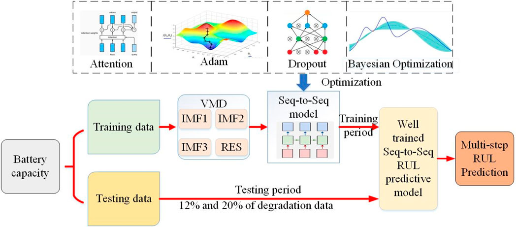
Considering the difficulty of predicting the life of a lithium battery at an early stage and the low precision of multistep prediction, a new RUL prediction method based on the bidirectional LSTM (BiLSTM) model and variational mode decomposition (VMD) is proposed herein. First, the SOH sequence of the battery is obtained using variational modes that effectively decompose the SOH degradation trend into various eigenmode components. Second, the MC algorithm is used to characterize the model uncertainty, and the confidence interval of the prediction is given. Finally, using the predicted SOH values, the predictions are iterated up to the battery failure threshold. Experiments were performed to show that the proposed RUL predictive neural network model achieves the lifetime prediction of lithium-ion batteries with only 12% capacity data. The results based on two lithium battery datasets from NASA and the University of Maryland show that the aging data of lithium-ion batteries can truly reflect the capacity decay process and that the proposed algorithm has high accuracy and robustness for early prediction of the RULs of lithium-ion batteries.

The remainder of this paper is structured as follows. Section 2 introduces the relevant algorithms; Section 3 introduces the battery data and pretreatment methods in detail along with the complete experimental process of variable lithium-ion battery aging data, results of the proposed RUL prediction method, and the specific evaluation criteria used; Section 4 finally presents the conclusions of this study.

2 Methodology

2.1 VMD

VMD is an adaptive, completely non-recursive modal transformation and signal processing technique. It improves the end effects as well as modal component localization of empirical mode decomposition (EMD) and has a more solid mathematical basis. Given time series with high complexity and strong non-linearity, it can reduce the non-stationarity of the signal and decompose it into relatively stable subsequences containing multiple frequency scales, which is suitable for signal extraction from non-stationary sequenced. The essence of the variational problem is the maximum value problem of the functional, and its core is to obtain n modal components u_n(t) while minimizing the sum of the bandwidths of each mode and ensuring that the sum of the modes is equal to the input signal f. The constrained variational model is shown in Equation 1:

$\left\{\begin{array}{l}{\displaystyle \underset{\left\{u_n\right\},\left\{w_n\right\}}{\min }}\left\{{\displaystyle \sum _n}{‖{\mathrm{\partial }}_t\left[\left(\delta \left(t\right)+j/\pi t\right)\times u_n\left(t\right)\right]e^{-j{w}_{n}t}‖}_2^2\right\},\\ s.t.{\displaystyle \sum _n}{u}_n=f\end{array}\right.(1)$

where ${\mathrm{\partial }}_t$ is the partial derivative of t, and $\delta \left(t\right)$ is the impulse function. The VMD algorithm introduces a quadratic penalty term and Lagrange multiplication operator, where the former ensures the reconstruction accuracy of the signal and the latter enhances the effects of the constraint conditions. The augmented Lagrange function is as shown below.

$\begin{array}{l}L\left(\left\{u_n\right\},\left\{w_n\right\},\lambda \right)=\alpha {\displaystyle \sum _n}{‖{\mathrm{\partial }}_t\left[\left(\delta \left(t\right)+j/\pi t\right)\times u_n\left(t\right)\right]e^{-j{w}_{n}t}‖}_2^2\\ +{‖f\left(t\right)-{\displaystyle \sum _n}{u}_n\left(t\right)‖}_2^2+〈\lambda \left(t\right),f\left(t\right)-{\displaystyle \sum _n}{u}_n\left(t\right)〉.\end{array}(2)$

The solution of the minimization problem in Equation 2 is the saddle point in Equation 3. Here, the alternating direction method of multipliers (ADMM) is used to solve the variational problem by updating u_n^k+1, w_n^k+1, and λ^k+1 to find the saddle point of the augmented Lagrangian function and use the Parseval/Plancherel Fourier isometric transformation to convert to the frequency domain to obtain the modal component u_n.

${\widehat{u}}_n^{k+1}\left(w\right)=\frac{\widehat{f}\left(w\right)-{\displaystyle \sum _{i\ne n}}{\widehat{u}}_i\left(w\right)+\frac{\widehat{\lambda }\left(w\right)}{2}.}{1+2\alpha {\left(w-w_n\right)}^2}(3)$

Similarly, the update method for the center frequency is given by Equation 4, and the updated value is according to Equation 5 until convergence to meet Equation 6 before obtaining the n modal components.

$w_n^{k+1}=\frac{{\int }_0^{\infty }w{\left|{\widehat{u}}_n\left(w\right)\right|}^{2}dw}{{\int }_0^{\infty }{\left|{\widehat{u}}_n\left(w\right)\right|}^{2}dw}.(4)$

${\widehat{\lambda }}^{k+1}\left(w\right)={\widehat{\lambda }}^k\left(w\right)+\tau \left({\widehat{f}}^k\left(w\right)-{\displaystyle \sum _n}{\widehat{u}}_n^{k+1}\left(w\right)\right).(5)$

${\displaystyle \sum _n}{‖u_n^{k+1}-u_n^k‖}_2^2/{‖u_n^k‖}_2^2<\epsilon (6)$

2.2 BiLSTM

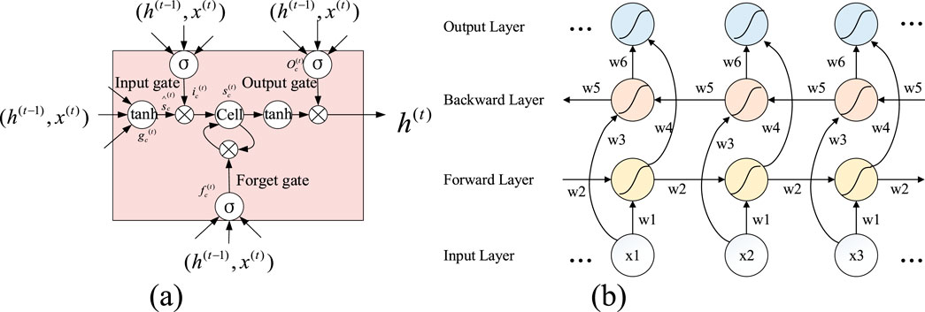
LSTM is no longer an ordinary hidden node but a storage unit with memory that can effectively avoid gradient distortion or explosion after a lengthy time sequence to overcome the difficulties associated with traditional RNN training. The key to LSTM is in the cell state and various gate structures, including the forget, input, and output gates. The unit state can store historical information and update it through continuous transmission. Therefore, the unit state can be regarded as the “memory” of the network. The illustrative structure of the LSTM predictor is shown in Figure 1A.

$i_c^{\left(t\right)}=\sigma \left(W_i\cdot \left[h^{\left(t-1\right)},x_t\right]+b_i\right).(7)$

$f_c^{\left(t\right)}=\sigma \left(W_f\cdot \left[h^{\left(t-1\right)},x_t\right]+b_f\right).(8)$

$o_c^{\left(t\right)}=\sigma \left(W_o\cdot \left[h^{\left(t-1\right)},x_t\right]+b_o\right).(9)$

${\stackrel{\wedge }{s}}_c^{\left(t\right)}=\mathit{tanh}(W_C\cdot \left[h^{\left(t\right)},x_t\right]+b_C.(10)$

$S_c^{\left(t\right)}=f_c^{\left(t\right)}\times S_c^{\left(t-1\right)}+i_c^{\left(t\right)}\times {\stackrel{\wedge }{s}}_c^{\left(t\right).}(11)$

$h^{\left(t\right)}=o_c^{\left(t\right)}·\mathit{tanh}\left(S_c^{\left(t\right)}\right).(12)$

Figure 1

Figure 1. Structures of the (A) LSTM network and its (B) Bi-LSTM variant.

In the above expressions, h and x represent the output and input samples of the network; o, i, and f represent the three gates mentioned above; matrices W and b indicate the weight parameters and bias terms, respectively; S represents the cell state; σ(·) is the ReLU activation function. From Equations 7–12, the error and weight of each LSTM neuron in the backpropagation process are calculated to update the network data and the output of the LSTM model. The number of neurons is directly proportional to the computing power and complexity of the neural network. In addition, because the number of network parameters is determined by the number of neurons in each layer, increasing the number of hidden layers will geometrically increase the number of parameters to be trained, and the corresponding complexity would be several times that of increasing the number of neurons in a single layer. To solve the above problems, the BiLSTM network model is considered as it not only avoids manual addition of the time frames but also captures the information of future states. The BiLSTM network is composed of forward and backward LSTM networks; it can not only obtain the past information of the input data but also use the future information and is very helpful for sequence data tasks.

As seen from Figure 1B, the BiLSTM network is composed of an input layer, a forward hidden layer, a backward hidden layer, and an output layer. The input layer receives a series of input data that are then applied to the forward and backward hidden layers to pay attention to both the upper and lower sequence information at the same time. The forward hidden layer is the forward flow of the LSTM from start to end, and the backward hidden layer is the reverse flow of the LSTM from end to start. The inputs to the output layer nodes are composed of the outputs of the backward and forward hidden layers to produce the final output sequence. In the structure, w1 and w3 are the weights from the input layer to the forward and backward hidden layers, w2 and w5 are the weights from the hidden layer to itself, and w4 and w6 are the weights from the forward and backward hidden layers to the output layer, respectively. The mathematical expressions are shown in Equations 13–15:

${\overrightarrow{h}}_t=LSTM\left(x_t,\overrightarrow{h_{t-1}}\right).(13)$

$\stackrel{⃖}{h_t}=LSTM\left(x_t,\stackrel{⃖}{h_{t-1}}\right).(14)$

$y_t=f\left(W_{\overrightarrow{h}}\overrightarrow{h_t}+W_{\stackrel{⃖}{h}}\stackrel{⃖}{h_{t-1}}+b\right).(15)$

The forward hidden layer reads the data in temporal order, passes the information forward along the temporal starting point, and obtains the prior information of the sequence. The backward hidden layer transmits the information in reverse to obtain the sequence information. By combining the forward and backward layer states at a given time as the output state of the hidden layer representing the contextual information of the sequence, this structure ensures that the BiLSTM can obtain the past and future information simultaneously. There is no information flow between the forward and backward hidden layers. The output of the forward LSTM is transmitted only to the forward LSTM unit, while the output of the reverse LSTM is transmitted only to the reverse LSTM unit, thus ensuring that the expanded map is non-cyclic. Although there is no connection between the two directions of the BiLSTM, the final output state sequence contains the temporal context information because the hidden layers jointly synthesize the output.

2.3 MC simulation

MC algorithms are generally divided into three stages as follows: constructing random probabilities, sampling from the constructed random probability distribution, and solving the estimator. Constructing a random probabilistic process for the problem that itself has a random quality necessitates accurate description and simulation of the probabilistic process. For deterministic problems that are not inherently random, such as the calculation of definite integrals, an artificial probability process must be constructed in advance; some of its parameters would then be the exact solutions to the required problem such that the problem without random properties can be transformed into one with random properties. Sampling and generating random variables from known probability distributions is essential to the MC approach because different probabilistic models can be regarded as composites of various probability distributions. In such examples, the simplest and most basic uniform distribution over (0,1) is used with random numbers being the key variables for the MC simulation. Once the estimator is solved through simulation, random variables are designated as the solutions to the required problem to ensure unbiased estimates. In this case, establishing an estimator is equivalent to examining the experimental results to obtain the problem solution. The advantages of the MC method are as follows: it is a statistical method that is relatively intuitive as well as easy to grasp and understand; it is easy to handle the random change characteristics of the load; it is easy to address various actual operational control strategies; the number of samples is independent of the scale of the system and is more advantageous for reliability evaluations of complex systems; it is easy to handle the operations of the system in chronological order.

Following the LSTM layer, the MC sampling method was introduced to generate multiple predictors using multiple samples. These multiple prediction samples generated by the MC layer are either averaged or weighted to obtain the final prediction of the RUL of the battery. The MC-BiLSTM network has the advantage of being able to account for the uncertainties in the battery life predictions to provide more accurate results. By combining the MC sampling and LSTM methods, the MC-BiLSTM network can better capture the long-term dependencies in time-series data and can weigh the different prediction samples to improve prediction accuracy.

3 Results and discussion

As more number of decay features are selected, the model construction becomes more difficult and calculations become more complicated. Too many decay features also increase the model complexity, causing overfitting and decreasing the prediction accuracy. In this work, the number of cycles is used to describe the decay process of a lithium battery. The values of each of the features of lithium battery decay are different in the order of magnitude. Through normalization, the features of different dimensions are converted into dimensionless isochronous data samples, so that the data of different dimensions have smaller values in similar ranges, thereby avoiding large data inputs to the network and resulting in large gradient updates to the network; this prevents convergence of the network and slows learning. The formula for normalization is shown in Equation 16

${x_t}^{*}=\frac{x_t-x_{\mathit{min}}}{x_{\mathit{max}}-x_{\mathit{min}},}(16)$

where $x_t$ are the original data; $x_{\mathit{min}}$ is the minimum value of the original data; $x_{\mathit{max}}$ is the maximum value of the original data. The optimal fusion feature of a lithium battery can be divided into three parts as the training, verification, and test sets. The first 70% of the data are defined as the training set, and the model is trained through repeated learning and memorization. The next 20% of the data constitute the verification set, which is used to evaluate the quality of early training. The last 10% of the dataset is used as the test set to assess the model. The model structure of the VMD-MC-BiLSTM network is shown in Figure 2. Two datasets are employed for training and testing the VMD-MC-BiLSTM model, which is optimized using Adam and the adaptive superparameter method. The adaptive superparameter method is based on Bayesian optimization and automatically filters the set of candidate superparameters that meet the learning objective task from the initial set of superparameters. Therefore, the proposed model is less sensitive to abnormal capacity values and deeply understands the degradation trends. Note that the network performance is sensitive to the number of neurons and dropout values. The ranges of values for the neurons and dropout are set to 10–200 and 0–0.5, respectively. Thus, the wide search space allows the BiLSTM to achieve better accuracy and robustness. Adaptive moment estimation (Adam) is a first-order optimization algorithm that replaces the traditional random gradient descent process and updates the neural network weights iteratively based on the training data. In addition, the attention mechanism allocates computing resources to more important tasks when there is limited computing power. Therefore, early prediction of the degradation pattern for a lithium-ion battery can be realized using the proposed model. Following feature selection and feature processing, the characteristics of the lithium battery are obtained. Next, the data are input to the LSTM network as a time series, and the capacity ratio is used as the prediction label. Lastly, these data are input to the written program simultaneously, and the dataset is divided before obtaining the predictions and results.

Figure 2

Figure 2. Structure of the model proposed in this work.

The optimizer updates the weight coefficients and provides the gradients of the weight updates, namely, the directions and sizes. Using a reasonable optimizer allows accelerated convergence of the network to obtain the global optimal solution. The activation function is used to increase the non-linearity of the entire network in terms of the expression or abstraction ability so that the network can learn the deeper contents of the data. The commonly used activation functions include the sigmoid, ReLU, and tanh functions. The number of layers in the network as well as the number of neurons in each layer can affect the model performance. Existing studies have shown that when a network has three or four layers, the model loss is small; when the network has more than four layers, the model loss will increase greatly, and the model performance will decline with increasing number of neurons. The main utility of the loss function is to supervise the learning process of the neural network. Theoretically, when there are more number of iterations of the neural network during training, the loss function value will be smaller. However, neural networks have strong learning abilities, and too many iterations can cause the network to only learn the relationships between the training set labels and true values, thus reducing the generalization of the prediction model; this produces good network predictions for the training set but poor results with the verification set. Therefore, during actual training of the model, a large number of iterations can lead to overfitting and poor prediction results.

The simulations in this study were conducted on a system with an Intel Core i7-8700 K CPU and NVIDIA GeForce GTX 1660ti independent graphics card using Windows 10 operating system and the TensorFlow deep-learning framework. The hybrid model structure used in the experiment consists of an input layer, a BiLSTM layer incorporating the attention mechanisms, a two-layer MC dropout random layer, a fully connected layer, and an output layer. After establishing the model, it is necessary to determine the loss function for network training to obtain the neural network parameters. In our experiments, the mean absolute error (MAE) was used as the loss function and Adam was used as the adaptive optimizer to minimize the objective function. The batch size was set to 16, and the number of epochs was set to 300.

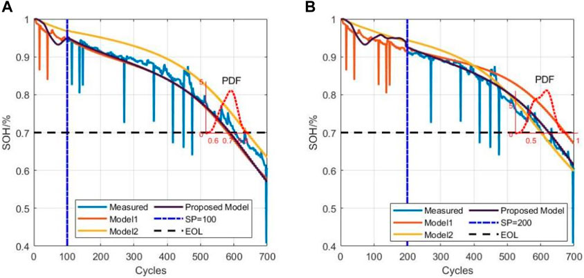
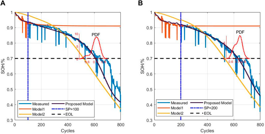
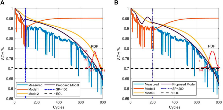
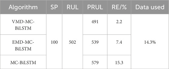
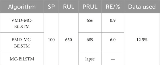
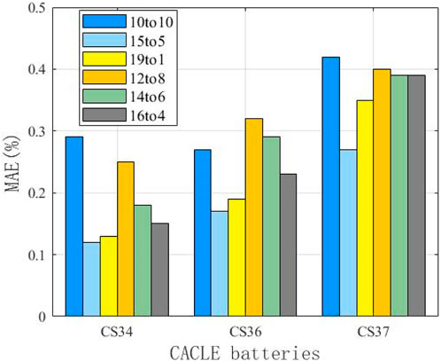
In this study, the end of life (EOL) point for each battery was considered the point at which the battery capacity dropped to 70% of its nominal value in the University of Maryland dataset. The datasets of five cells at different current rates and cutoff voltages were used to verify the proposed model. Early identification results of the battery degradation patterns based on our approach are shown in Figures 3–5. Here, CS33, CS35, and CS38 were used for training, while CS34, CS36, and CS37 were used for testing. The hyperparameter values of the number of BiLSTM units shown in the random search are 10–200, step size is 10, and dropout values are [0.1, 0.2, 0.3, 0.4, 0.5]. Based on the results of the KerasTuner search, the final hyperparameters selected were as follows: number of BiLSTM cells is 80, random discard rate is 0.4, window size is [15,1], and result shape is [5,1]. The model was trained once the hyperparameters were determined. In addition, three comparison models are defined as Model 1, Model 2, and Model 3. Among these, Model 1 was trained using raw data, namely, the MC-BiLSTM model; Model 2 was trained on the EMD data, namely, the EMD-MC-BiLSTM model; Model 3 was trained on the VMD data, namely, the VMD-MC-BiLSTM model. The experiments assessed the trends of the RULs predicted from the first 12% start point (SP) of the lithium battery lifecycle and from 20%. Tables 1–3 list the prediction performances of the CS34, CS36, and CS37 batteries with the three models, respectively. Among these, the predictions after VMD are observed to better fit the degradation trends of the original data and achieve the minimum error value. However, some RUL predictions trained with raw data do not show degradation trends; one possible reason for this is that the raw data are too noisy and that the training model does not converge well. For the CS34 batteries, the EOL point is 602 cycles, and the early SP predicted from 100 results in a true RUL of 502 and average predicted RUL (PRUL) of 491; both these values are within the 95% confidence interval (CI) of PRUL, which is [313, 690]. When forecasting from an early SP of 200, the true RUL is 402, average PRUL is 392, and 95% CI of PRUL is [360, 444]. For the CS36 batteries, the EOL point is 610 cycles, and the early SP predicted from 100 results in a true RUL of 510 and average PRUL of 462, with both values falling within the 95% CI of PRUL of [368, 554]. When predicting from an early SP of 200, the true RUL is 410, average PRUL is 420, and 95% CI of PRUL is [344, 497]. Similarly, for the CS37 batteries, the EOL point is 750 cycles, and the early SP predicted from 100 gives a true RUL of 650, average PRUL of 656, and 95% CI of PRUL of [604, 707]. When forecasting from an early SP of 200, the true RUL is 550, average PRUL is 572, and 95% CI of PRUL is [526, 620]. Figure 6 compares the effects of different sliding window sizes on the model, particularly those for 10 to 10, 15 to 5, 19 to 1, 12 to 8, 14 to 6, and 16 to 4 sequence lengths. The estimated errors were low for the three test cells, and the prediction error of the 15 to 5 sequence was minimal for the CALCE dataset. Table 4 shows the predictions for the CS34, CS36, and CS37 batteries when the predicted values for SP = 100 (12%) and SP = 200 (20%) are very close to the actual values.

Figure 3

Figure 3. Prediction results of CS34 from the (A) 100th and (B) 200th cycles.

Figure 4

Figure 4. Prediction results of CS36 from the (A) 100th and (B) 200th cycles.

Figure 5

Figure 5. Prediction results of CS37 from the (A) 100th and (B) 200th cycles.

Table 1

Table 1. Comparison of the prediction accuracies of different algorithms for CS34.

Table 2

Table 2. Comparison of the prediction accuracies of different algorithms for CS36.

Table 3

Table 3. Comparison of the prediction accuracies of different algorithms for CS37.

Figure 6

Figure 6. Comparison of the prediction accuracies for different sequence lengths.

Table 4

Table 4. Accuracies of different prediction starting points for batteries from the University of Maryland dataset.

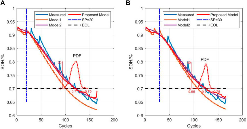
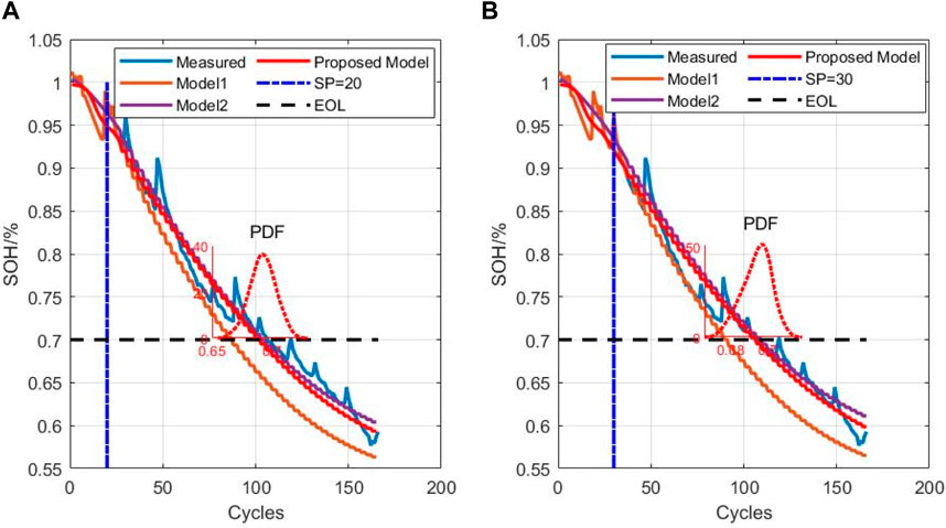
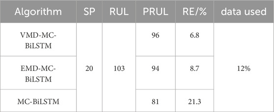
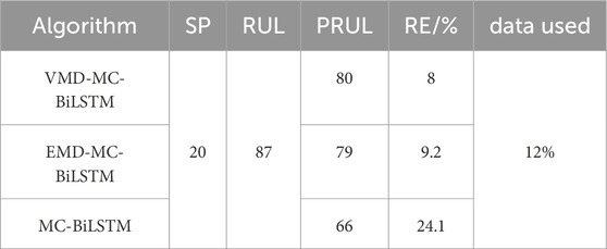
From the NASA dataset, information on batteries B5 and B6 was used for testing, while B7 and B18 were used for training; in the NASA dataset, the EOL point for each battery was set at 70% of the nominal capacity. Figures 7, 8 show the RUL forecast results for B5 and B6 from the NASA dataset. The RUL forecast relative errors (REs) for B5 are 6.8% and 3.2% when forecasting from cycles 20 and 30, respectively; this indicates that the model predictions are more accurate when there is a greater amount of prior capacity data. Specifically, the EOL point of B5 is 123, and the true RUL is 103 when the SP is 20; this result is within the 95% CI of PRUL of [84,107], indicating that the prediction is more accurate and highly reliable. When the SP is 30, the true RUL is 93, which is within the 95% CI of PRUL of [80,100], indicating that the initial EOL diagnosis is relatively accurate with high reliability. Similarly, when forecasting from the 20th and 30th cycles, the REs of B6 are 8.0% and 2.6%, respectively. The EOL of B6 is 107, and this service life is slightly lower than that of B5, which is attributable to inconsistencies caused by the manufacturing, equipment, and other links. Further analysis of B6 shows that when the prediction starts from the 20th cycle, the actual RUL is 87, which is within the 95% CI of PRUL of [70,88]; when the prediction starts from the 30th cycle, the actual RUL is 77, which is within the 95% CI of PRUL of [67,84]. For the NASA dataset, we observe from the figures that the prediction and regression effects of the post-EMD and -VMD data are similar because the original data itself are not very noisy. Figure 9 shows a comparison of the predictions for different sliding window sequence lengths; as noted from the figure, the optimal sequence length is 7 to 3 for the NASA dataset. For B5, the MAE values are 0.0122, 0.0120, 0.0126, and 0.0127 when the sequence lengths are 9 to 1, 8 to 2, 6 to 4, and 5 to 5, respectively. For B6, the MAE values are 0.0138, 0.0141, 0.0144, and 0.0146 when the sequence lengths are 9 to 1, 8 to 2, 6 to 4, and 5 to 5, respectively. When the sequence length is too small or too large, the RUL prediction accuracy will be lower or even invalid. Table 5 shows the RUL forecast performances for different SPs of batteries B5 and B6. The predicted values at SP = 20 (12%) and SP = 30 (20%) are very close to the actual values, indicating that the proposed method can effectively diagnose the RULs of batteries at the early stages. Tables 6, 7 show the predictions for batteries B5 and B6 based on the three algorithms; it can be seen that the predictions with VMD have the smallest REs.

Figure 7

Figure 7. Prediction results of B5 from the (A) 20th and (B) 30th cycles.

Figure 8

Figure 8. Prediction results of B6 from the (A) 20th and (B) 30th cycles.

Figure 9

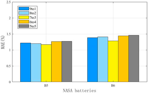
Figure 9. Comparison of the prediction accuracies for different sequence lengths of the batteries from the NASA dataset.

Table 5

Table 5. Prediction accuracies for different starting points for batteries B5 and B6.

Table 6

Table 6. Comparison of the prediction accuracies of different algorithms for B5.

Table 7

Table 7. Comparison of the prediction accuracies of different algorithms for B6.

4 Conclusion

The remaining life of a lithium battery was predicted in this work based on the VMD-MC-BiLSTM network using early-stage battery capacity data. The following are the conclusions of this study. We successfully applied the VMD-MC-BiLSTM network to predict the remaining life of lithium battery and achieved satisfactory results. Compared to traditional statistics-based methods or traditional deep-learning models, the VMD-MC-BiLSTM network produces better results from processing sequential data, especially with regard to capturing long-term dependencies and processing variable-length sequences. Our experimental results show that the VMD-MC-BiLSTM network not only effectively captures the dynamic characteristics of lithium batteries during operation but also provides accurate predictions of their RULs. In addition, we conducted in-depth analyses and optimization of the VMD-MC-BiLSTM network with regard to the network structure design, hyperparameter adjustment, and training strategy. Through these optimization measures, we further improved the predictive performance of the model, making it more suitable for application to actual lithium battery health management systems. Despite the encouraging results, some challenges remain and further improvements are possible. For example, the present study is mainly based on datasets of a specific type of lithium battery, and further validation and model adjustment may be required for different types of lithium batteries or different working conditions. In addition, the performance of our model in handling abnormal or extreme conditions needs to be improved, which may require the introduction of more anomaly detection mechanisms or complex structural design of the model. In summary, the RUL prediction of a lithium battery based on the VMD-MC-BiLSTM network has great significance for improving the efficiency and accuracy of a lithium battery health management system. Future research on this subject may need to consider broader data validations, further optimizations of the model, as well as validation and iteration in practical applications to drive further developments.

Data availability statement

Publicly available datasets were analyzed in this study. These data can be found here: https://calce.umd.edu/data#CS2.

Author contributions

MG: writing–original draft, writing–review and editing, conceptualization, data curation, formal analysis, funding acquisition, investigation, methodology, project administration, resources, software, supervision, validation, and visualization. LZ: writing–original draft and writing–review and editing. MZ: writing–original draft and writing–review and editing.

Funding

The authors declare that no financial support was received for the research, authorship, and/or publication of this article.

Conflict of interest

Author MG was employed by Shenhua Group Zhungeer Energy Co., Ltd. Authors LZ and MZ were employed by Qingdao Wohua Soft Control Co., Ltd.

Publisher’s note

All claims expressed in this article are solely those of the authors and do not necessarily represent those of their affiliated organizations or those of the publisher, editors, and reviewers. Any product that may be evaluated in this article or claim that may be made by its manufacturer is not guaranteed or endorsed by the publisher.

References

Ansari, S., Ayob, A., Hossain Lipu, M. S., Hussain, A., and Saad, M. H. M. (2022). Remaining useful life prediction for lithium-ion battery storage system: a comprehensive review of methods, key factors, issues and future outlook. Energy Rep. 8, 12153–12185. doi:10.1016/j.egyr.2022.09.043

CrossRef Full Text | Google Scholar

Bao, Z., Nie, J., Lin, H., Jiang, J., He, Z., and Gao, M. (2023). A global–local context embedding learning based sequence-free framework for state of health estimation of lithium-ion battery. Energy 282, 128306. doi:10.1016/j.energy.2023.128306

CrossRef Full Text | Google Scholar

Chen, D., Hong, W., and Zhou, X. (2022). Transformer network for remaining useful life prediction of lithium-ion batteries. IEEE Access 10, 19621–19628. doi:10.1109/access.2022.3151975

CrossRef Full Text | Google Scholar

Ding, P., Liu, X., Li, H., Huang, Z., Zhang, K., Shao, L., et al. (2021). Useful life prediction based on wavelet packet decomposition and two-dimensional convolutional neural network for lithium-ion batteries. Renew. Sustain. Energy Rev. 148, 111287. doi:10.1016/j.rser.2021.111287

CrossRef Full Text | Google Scholar

Guha, A., and Patra, A. (2018). Online estimation of the electrochemical impedance spectrum and remaining useful life of lithium-ion batteries. IEEE Trans. Instrum. Meas. 67 (8), 1836–1849. doi:10.1109/tim.2018.2809138

CrossRef Full Text | Google Scholar

He, W., Williard, N., Osterman, M., and Pecht, M. (2011). Prognostics of lithium-ion batteries based on Dempster-Shafer theory and the Bayesian Monte Carlo method. J. Power Sources 196 (23), 10314–10321. doi:10.1016/j.jpowsour.2011.08.040

CrossRef Full Text | Google Scholar

Jiang, H., Lv, X., and Wang, K. (2024). Application of triboelectric nanogenerator in self-powered motion detection devices: a review. Apl. Mater. 12 (7). doi:10.1063/5.0219633

CrossRef Full Text | Google Scholar

Kim, S., Choi, Y. Y., Kim, K. J., and Choi, J. I. (2021). Forecasting state-of-health of lithium-ion batteries using variational long short-term memory with transfer learning. J. Energy Storage 41, 102893. doi:10.1016/j.est.2021.102893

CrossRef Full Text | Google Scholar

Li, P., Zhang, Z., Xiong, Q., Ding, B., Hou, J., Luo, D., et al. (2020). State-of-health estimation and remaining useful life prediction for the lithium-ion battery based on a variant long short term memory neural network. J. power sources 459, 228069. doi:10.1016/j.jpowsour.2020.228069

CrossRef Full Text | Google Scholar

Lipu, M. H., Karim, T., Ansari, S., Miah, M., Rahman, M., Meraj, S., et al. (2023). Intelligent SOX estimation for automotive battery management systems: state-of-the-art deep learning approaches, open issues, and future research opportunities. Energies 16 (1), 23. doi:10.3390/en16010023

CrossRef Full Text | Google Scholar

Liu, Y., Li, Q., and Wang, K. (2024). Revealing the degradation patterns of lithium-ion batteries from impedance spectroscopy using variational auto-encoders. Energy Storage Mater. 69, 103394. doi:10.1016/j.ensm.2024.103394

CrossRef Full Text | Google Scholar

Ma, G., Zhang, Y., Cheng, C., Zhou, B., Hu, P., and Yuan, Y. (2019). Remaining useful life prediction of lithium-ion batteries based on false nearest neighbors and a hybrid neural network. Appl. Energy 253, 113626. doi:10.1016/j.apenergy.2019.113626

CrossRef Full Text | Google Scholar

Montaru, M., Fiette, S., Koné, J. L., and Bultel, Y. (2022). Calendar ageing model of Li-ion battery combining physics-based and empirical approaches. J. Energy Storage 51, 104544. doi:10.1016/j.est.2022.104544

CrossRef Full Text | Google Scholar

Patil, M. A., Tagade, P., Hariharan, K. S., Kolake, S. M., Song, T., Yeo, T., et al. (2015). A novel multistage Support Vector Machine based approach for Li ion battery remaining useful life estimation. Appl. Energy 159, 285–297. doi:10.1016/j.apenergy.2015.08.119

CrossRef Full Text | Google Scholar

Qi, G., Ma, N., and Wang, K. (2024). Predicting the remaining useful life of supercapacitors under different operating conditions. Energies 17 (11), 2585. doi:10.3390/en17112585

CrossRef Full Text | Google Scholar

Razavi-Far, R., Chakrabarti, S., and Saif, M. (2017). “Multi-step parallel-strategy for estimating the remaining useful life of batteries[C],” in 2017 IEEE 30th Canadian conference on electrical and computer engineering (CCECE). IEEE, 1–4.

CrossRef Full Text | Google Scholar

Richardson, R., Osborne, M. A., and Howey, A. (2017). Gaussian process regression for forecasting battery state of health. J. Power Sources 357, 209–219. doi:10.1016/j.jpowsour.2017.05.004

CrossRef Full Text | Google Scholar

Sarasketa-Zabala, E., Martinez-Laserna, E., Berecibar, M., Gandiaga, I., Rodriguez-Martinez, L., and Villarreal, I. (2016). Realistic lifetime prediction approach for Li-ion batteries. Appl. energy 162, 839–852. doi:10.1016/j.apenergy.2015.10.115

CrossRef Full Text | Google Scholar

Takyi-Aninakwa, P., Wang, S., Zhang, H., Yang, X., and Fernandez, C. (2023). A hybrid probabilistic correction model for the state of charge estimation of lithium-ion batteries considering dynamic currents and temperatures. Energy 273, 127231. doi:10.1016/j.energy.2023.127231

CrossRef Full Text | Google Scholar

Wei, J., Dong, G., and Chen, Z. (2017). Remaining useful life prediction and state of health diagnosis for lithium-ion batteries using particle filter and support vector regression. IEEE Trans. Industrial Electron. 65 (7), 5634–5643. doi:10.1109/tie.2017.2782224

CrossRef Full Text | Google Scholar

Zhang, Y., Xiong, R., He, H., and Pecht, M. G. (2018). Long short-term memory recurrent neural network for remaining useful life prediction of lithium-ion batteries. IEEE Trans. Veh. Technol. 67 (7), 5695–5705. doi:10.1109/tvt.2018.2805189

CrossRef Full Text | Google Scholar

Zhu, C., Gao, M., He, Z., Wu, H., Sun, C., Zhang, Z., et al. (2023a). State of health prediction for li-ion batteries with end-to-end deep learning. J. Energy Storage 65, 107218. doi:10.1016/j.est.2023.107218

CrossRef Full Text | Google Scholar

Zhu, C., He, Z., Bao, Z., Sun, C., and Gao, M. (2023b). Prognosis of lithium-ion batteries’ remaining useful life based on a sequence-to-sequence model with variational mode decomposition. Energies 16 (2), 803. doi:10.3390/en16020803

CrossRef Full Text | Google Scholar

Zhu, C., Zheng, B., He, Z., Gao, M., Sun, C., and Bao, Z. (2021). State of health estimation of lithium-ion battery using time convolution memory neural network. Mob. Inf. Syst. 2021, 1–16. doi:10.1155/2021/4826409

CrossRef Full Text | Google Scholar