The expected solar performance and ramp rate tool: a decision-making tool for planning prospective photovoltaic systems

The Expected Solar Performance and Ramp Rate tool (ESPRR) is an open-source interactive web-based application that reliably calculates ramp rate (RR) statistics and an expected power generation time series for prospective photovoltaic (PV) systems. Users create PV systems by defining site parameters. ESPRR uses those parameters with irradiance data from the National Solar Radiation Database (NSRDB) to create a time series of power output from which RR statistics are calculated. This study rigorously evaluates ESPRR’s performance using 5 years of measured power output from a fleet of utility-scale systems and finds that ESPRR calculates stress-case RRs within an error of 0.05 MW/min and 0.42 MW/min for the worst-case RRs. We evaluate the expected AC power output in clear-sky conditions and find an NRMSE of less than 10% and an NMBE of less than 6% for the fleet’s largest system. The NRMSE is 10%–15% of system capacity for non-clear-sky conditions, and the NMBE is about zero. The evaluation shows that ESPRR can estimate PV output and RRs that are representative of operational systems, meaning users can use the results from ESPRR in the decision-making process for designing new systems or when adding systems to an existing fleet. Since only system parameters are required to site a proposed system anywhere on a map, users can site and reposition a fleet of PV systems in a way that reduces significant RRs. As the grid-tied PV capacity continues to increase, the mitigation of significant RRs grows in importance. ESPRR can help developers and utilities create geographically diverse fleets of PV systems that will promote grid reliability and avoid significant RRs. ESPRR source code is available at https://github.com/UARENForecasting/ESPRR.

1 Introduction

A ramp rate (RR) can be defined as a difference in power production from one time to another. Shadows from passing clouds cause intra-day variations in solar irradiance that can result in a significant RR in power production from photovoltaic (PV) systems. A lack of geographic diversity in PV generation sites exacerbates fleet-wide RRs because sites within a certain location will experience weather conditions at similar times. However, a geographically diverse fleet will experience weather conditions at different times, resulting in a lesser magnitude RR in the aggregated output (Hossain and Ali 2014; Mills and Wiser 2011).

The continued increase of PV penetration to the grid across the United States raises questions about power systems’ flexibility and ability to deliver reliable, high-quality power under variable weather conditions if fleets of systems are geographically clustered. The installed capacity of utility-scale PV in the United States is projected to more than double from 2020 to 2030 (Bolinger et al., 2021). As the capacity increases, decisions about where to site new systems will only grow in importance. The availability and price of land are often drivers of where new systems will be sited. However, developers and utilities must prioritize geographic diversity within their fleets when positioning new systems to avoid significant RRs.

The estimation of the worst expected RRs from PV systems has been investigated. Jamaly et al. (2013) shows observed RRs from a fleet and used satellite-derived irradiance to verify RR 57 timing successfully. Wang et al. (2019) and Lappalainen et al. (2020) developed methodologies to 58 predict the worst expected RRs using cloud motion vectors, irradiance observations, and system 59 geometry at existing PV sites. These methods rely on observations that are not typically available at prospective sites for PV systems. The Expected Solar Performance and Ramp Rate tool (ESPRR) is a novel application that estimates RRs for proposed PV systems without needing additional observations valid for the proposed location. From user-specified system parameters only, ESPRR calculates an expected annual performance time series of power production and the proposed system’s stress- and worst-case RRs. ESPRR uses gridded observational irradiance data (NSRDB), meaning users can interactively site proposed PV systems anywhere on a geographical map. Multiple proposed systems can be grouped into a fleet, and their locations can subsequently be optimized to minimize RR statistics in the aggregated fleet output.

Co-located battery energy storage systems (BESS) can smooth PV power output and keep RRs within safe limits (Martins et al., 2019). For safe and efficient operations, system designers must understand the typical and extreme RRs a system will likely experience to optimize the size and cost of the BESS. ESPRR can provide the RR information that could be used to plan co-located PV-BESS. BESSs can also be used for load-shifting, where the storage system is charged during the day and dispatched when most needed, often after sunset. In this situation, ESPRR-derived RR information could be used to ensure that system infrastructure, such as voltage tolerances on distribution lines and inverters, can safely withstand the most extreme intra-day variations in irradiance. ESPRR could also be used alongside advanced energy management systems, such as the one described in Gheorghiu et al. (2024), to assess proposed PV systems’ financial viability and expected load requirements.

ESPRR was developed in collaboration with Salt River Project Agricultural Improvement and Power District (SRP), a utility company in the Southwest United States. However, ESPRR has broad applicability outside this region since the software draws from open-source packages, is publicly available (repository at https://github.com/UARENForecasting/ESPRR), and utilizes publicly available input data. An instance of ESPRR could quickly be deployed for any region in the contiguous United States by sub-setting the input data for a different region (different irradiance and weather data would need to be used for regions outside the US). This study evaluates the expected performance time series and RRs using power observations from a fleet of utility-scale PV solar sites in Arizona. The evaluation shows that the ESPRR-calculated expected performance time series and RR statistics represent the characteristics of operational PV systems and are valuable for the PV system design and planning process.

The remainder of this article is organized as follows: Section 2.1 gives an overview of ESPRR. Section 2.2 describes the user input information necessary to create a PV system in ESPRR. Section 2.3 outlines the computational process that generates the expected power time series and RR statistics. The methods to evaluate ESPRR’s output are shown in Section 3: evaluation site descriptions (Section 3.1), quality assurance methods for observational data (Section 3.2), error metric and confidence interval definitions (Sections 3.3, 3.4), clear-sky filtering methods (Section 3.5), and a description of weather in the context of climatology during the evaluation period (Section 3.6). The results are shown in Section 4, including the evaluations of RRs in Sections 4.1–4.3 and the expected performance evaluation in Section 4.4. Finally, the conclusions of this study are presented in Section 5.

2 ESPRR methodology

2.1 Overview of ESPRR

ESPRR is an open-source, interactive web application that calculates an expected power generation time series and stress- and worst-case RR statistics for proposed PV systems. It accounts for user-specified system location, size, orientation, and geographic extent. ESPRR allows users to group multiple systems into a fleet and then modify the location of the systems to minimize RRs in the total fleet output. ESPRR consists of a user-friendly web-based frontend backed by a REST API for computations.

2.2 User-defined inputs

To create a proposed PV system, users must first specify system parameters (e.g., total AC capacity, DC/AC ratio, and panel orientation for fixed-tilt systems or tracking parameters for a single-axis tracker). Users then site the new system on an interactive map; see Figure 1. The new system is initially represented by a square with an area corresponding to a DC capacity of 40 MW per km². However, the system can be reshaped into a rectangle by modifying the aspect ratio while maintaining the same density of modules. The new system can be relocated by dragging it across the map, and transmission lines can be overlaid onto the map (U.S. Department of Homeland Security and Oakridge National Lab 2023). A direct path to the closest transmission line can be toggled on and off, and additional information about the transmission line (e.g., distance to the line, owner, type of line, status, and valid date of the information) is available on-screen.

Figure 1

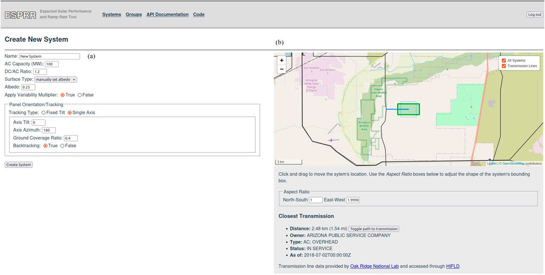
Figure 1. A screenshot from the ESPRR website on the Create New System page; (A) shows where users define new system parameters and (B) show the placement of the system (green) on the map and the aspect ratio of the new system. Transmission lines are overlaid on the map in black, the path from the new system to the transmission line in blue, and other additional transmission line information is shown below the map.

2.3 Computational process

2.3.1 Calculating expected power time series and ramp rates

PV system parameters are input to the NREL PVWatts module/inverter model chain within the python package pvlib (version 0.9.0, Holmgren et al., 2018). The model chain outputs a 5-min frequency time series of expected power generation using the system parameters and weather data. For weather data, ESPRR inputs gridded air temperature, wind speed, and clear-sky and all-sky solar irradiance datasets from the NREL National Solar Radiation Database (NSRDB) for 2018–2022 (Sengupta et al., 2018). The NSRDB irradiance dataset is a satellite-derived gridded estimate of observed irradiance with a 2 km grid spacing. (Yang 2021) evaluated NSRDB irradiance data at several SURFRAD sites for 2018 and 2019 and concluded that the 5-minute irradiance data are suitable for solar applications that require long-term data, such as PV system design, simulation, and performance evaluation. The NSRDB dataset is considered one of the best publicly available gridded representations of surface irradiance.

From the expected power generation time series, ESPRR calculates RRs as the difference in power generation across 5, 10, 15, 30, and 60-min periods. Statistics such as the stress-case RR up/down are represented by the 95th/5th percentile drawn from the distribution of RRs. For worst-case RRs up/down, the 99.99th/0.01st percentile is used. Typical sunrise/sunset ramps are also calculated using the same method but using clear-sky irradiance data and the 95th/5th percentile. Given a user selection, ramp statistics can be displayed as absolute ramps (MW) or RRs (MW/min). An interactive graphic of the expected power generation time series is shown (Figure 2, panel b), and the time series and ramp statistics are available for download in CSV format or optimized binary (Apache Arrow). These options make ESPRR easy to use and fit for various user applications.

Figure 2

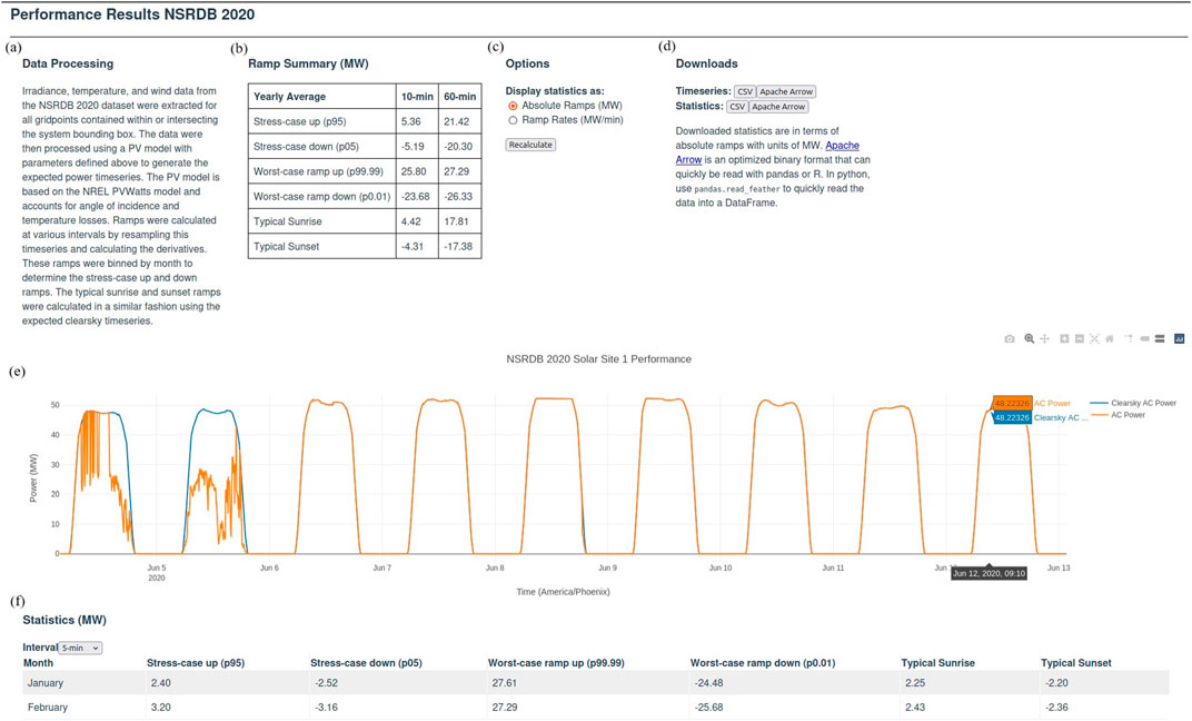
Figure 2. A screenshot from the ESPRR website on the Results page; (A) shows information about the data processing, (B) a table showing a summary of yearly average ramp statistics, (C) shows user selection of units of ramp statistics (MW) or (MW/min), (D) shows the download buttons for expected power generation time series from ESPRR and ramp statistics, (E) shows an interactive graphic of the expected power generation time series, and (F) shows a breakdown of the ramp statistics by month.

2.3.2 Grouping systems into a fleet

An important part of ESPRR’s value for planning decisions is the ability to group systems into a fleet, see Figure 3. With two or more systems made, users can create a group (fleet) for which an expected power generation time series and RR statistics will be calculated. The aggregation of proposed systems allows fleet-wide performance to be assessed. Users can then modify each system in terms of the location, size, and orientation to minimize RRs in total fleet output.

Figure 3

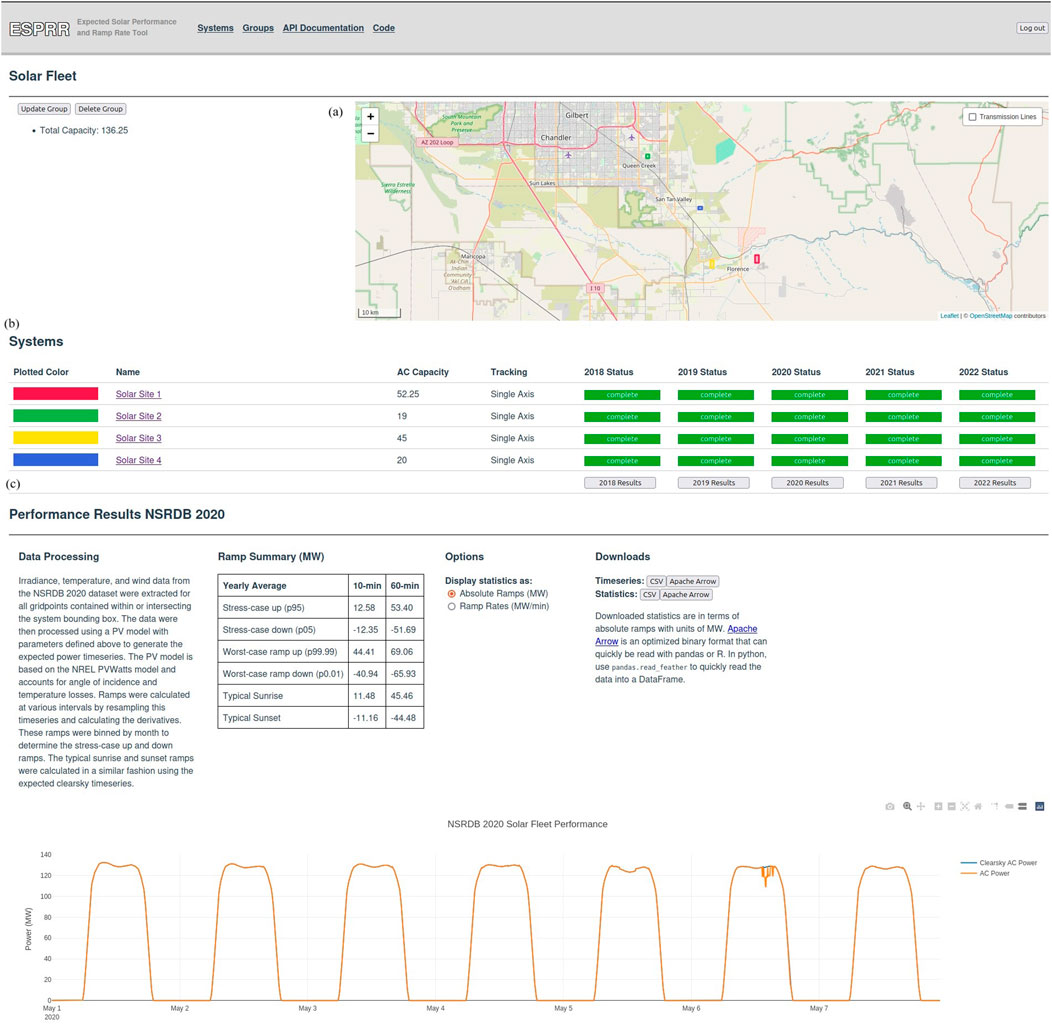
Figure 3. Screenshot from the ESPRR website on the Groups page; (A) shows the map with the systems in the fleet color-coded, (B) shows the systems that the fleet is comprised of and their associated parameters (AC capacity and tracker type) as well as the status of the calculations for each year and system. (C) Shows the performance results, similar to Figure 2, but for the aggregated group of systems.

Alternatively, a distributed group of systems can be auto-generated given a user-specified distance between systems and a placement strategy for the fleet, either a grid or line. The distributed group of systems can later be modified like an individual system. This system generation method is potentially useful for planning PV systems that will be co-located but operated independently and connected to the grid with separate points of interconnection.

2.3.3 Variability multiplier in cumulus cloud conditions

Initial tests showed that computed RRs could underestimate observed RRs during intermittent cloud conditions. To address this, we created an optional “Variability Multiplier” that modifies the ESPRR estimated power output and aims to better represent observed RRs during such conditions.

Figure 4A shows a time series of power generation from a PV system with varying cloud conditions each day in September 2019: a clear day (9/3), followed by 3 days with partial cloud coverage (9/4 through 9/6), an overcast day (9/7), and then a day with intermittent cloud conditions (9/8). On the days with intermittent clouds, e.g., September 8th, we see an underestimation of the intraday variability by comparing the observed power generation to the ESPRR estimate without the Variability Multiplier. During cloudy conditions, power generation is overestimated, which stems from an overestimation of surface irradiance in the input data. The clouds shown in the observed power generation are likely either misrepresented in terms of cloud optical thickness or are sub-grid-scale clouds that are missed in the irradiance data. The NSRDB irradiance data has a 2 km grid spacing, and cumulus clouds are often less than 2 km in size.

Figure 4

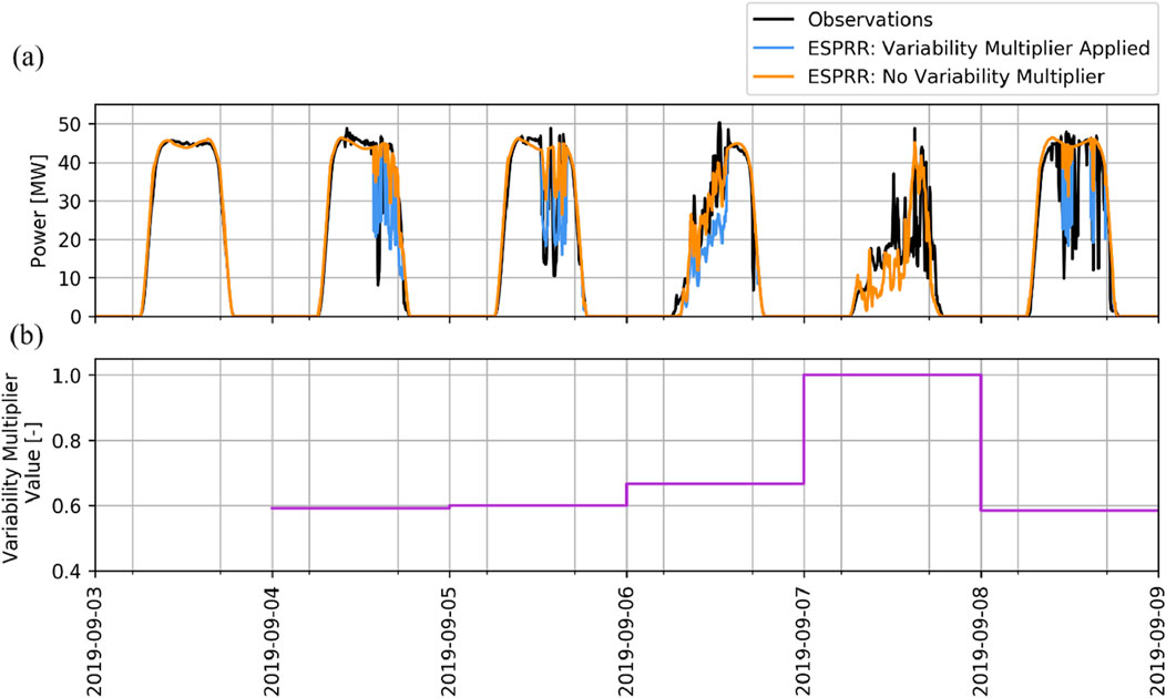
Figure 4. A time series showing (A) the expected power output calculated from ESPRR with (blue) and without (orange) the Variability Multiplier applied versus observations (black) and (B) the corresponding daily value of the Variability Multiplier (purple).

The Variability Multiplier (M) is defined as:

$M=1-0.5\left(\frac{s_d-s_{\mathit{min}}}{s_{\mathit{max}}-s_{\mathit{min}}}\right)(1)$

where $s_d$ is the standard deviation of power generation for the current day and $s_{\mathit{min}}/s_{\mathit{max}}$ are the yearly min/max daily standard deviation of power generation. The Variability Multiplier varies in magnitude since we want the greatest reductions in estimated power applied on the days with the greatest variability to better capture the magnitude of intra-day variability. Equation 1 shows M varies between 0.5 and 1 based on the daily standard deviation of power generation normalized over the year. Figure 4 panel (b) shows that the magnitude of the Variability Multiplier is greater on a day with less intraday variability (9/6) and lesser on days with greater variability (9/8).

As well as being variable in magnitude, the multiplier is conditional. The Variability Multiplier does not operate on clear-sky times (September 3rd) or overcast days with low irradiance (September 7th), where optically thick clouds cause daily generation to be less than half of clear-sky generation. While Figure 4 panel (a) shows that the application of the Variability Multiplier decreases the power estimate for non-clear times and suggests a better match to the observed variability of power production, a detailed evaluation of the distribution of RRs from ESPRR with and without the multiplier applied is presented in Section 4.1.

Another feature not represented by the irradiance data is over-irradiance, where additional irradiance is reflected downward toward the surface under a broken cloud field. Over-irradiance is a feature of observed irradiance time series’ that current datasets and radiation models cannot represent. Correcting the irradiance data for these errors is not possible without additional ground-based irradiance observations.

3 Evaluation methods

3.1 Description of sites used for evaluation

To evaluate ESPRR output, we use observed power generation data from 2018 through 2022 at four utility-scale SRP solar sites. Table 1 shows the site parameters used to create the PV systems.

Table 1

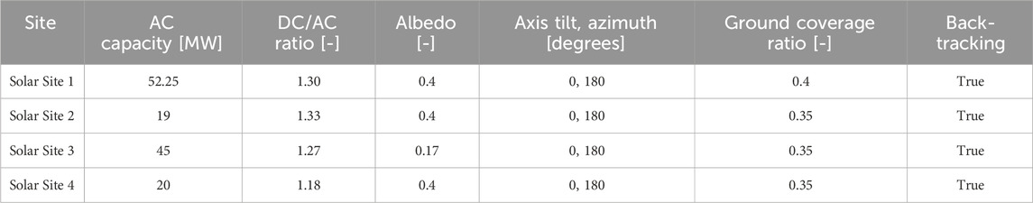
Table 1. System parameters for the four SRP sites used to evaluate ESPRR performance.

3.2 Quality assurance of observation data

The observed power generation data are quality-assured by removing known outages from the time series. Then, the observations pass through a zenith filter <90° to remove any erroneous non-zero values after sunset. A final filter removes any observations greater than the system’s capacity to mask out over-irradiance events from the statistical evaluation.

3.3 Error metrics

We use normalized root mean square error (NRMSE, %) and normalized mean bias error (NMBE, %) to quantify errors from observations:

$\text{NRMSE}=\frac{100}{norm}•\sqrt{\frac{1}{\mathrm{N}}{\displaystyle \sum _{\mathrm{i}=1}^{\mathrm{N}}}{\left({\mathrm{x}}_{\mathrm{i},\mathrm{e}}-{\mathrm{x}}_{\mathrm{i},\mathrm{o}}\right)}^2}(2)$

$\text{NMBE}=\frac{100}{norm}•\frac{1}{\mathrm{N}}{\displaystyle \sum _{\mathrm{i}=1}^{\mathrm{N}}}\left({\mathrm{x}}_{\mathrm{i},\mathrm{e}}-{\mathrm{x}}_{\mathrm{i},\mathrm{o}}\right)(3)$

where $x_{i,e}$, $x_{i,o}$ are the $i^{th}$ entry of the ESPRR estimate ($e$) and observation ($\mathrm{o}$), N is the length of the time series, and norm is the nameplate AC capacity of a PV system. We use SS_RMSE to evaluate RMSE skill from a reference method;

${SS}_{RMSE}=1-\frac{{RMSE}_{test}}{{RMSE}_{ref}}(4)$

for example, to compare the RMSE from ESPRR with (test) and without (ref) the Variability Multiplier applied.

3.4 Confidence interval calculations

We use the following method to calculate confidence intervals for the RR statistics, representing the sampling error and the system tolerance. We use a bootstrap randomization sampling strategy to quantify the sampling error, leaving out 10% of the distribution of RRs for each random sample. We repeat the percentile calculation for 500 iterations to create a distribution of percentiles. 95% confidence intervals are drawn from these distributions to estimate the sampling error.

To incorporate a representation of the system tolerance into the confidence interval, we add a factor of 10% of maximum plant generation per hour to the confidence intervals. The aim is to include a typical yet significant forecast error that a new system could experience and how that would modify the RR percentiles. As an example, for Solar Site 1 (52.25 MWp), the system tolerance added to the confidence interval is $\left(52.25•0.1\right)/60=0.09$ MW/min.

3.5 Clear-sky filtering for expected performance evaluation

For system planning purposes, we are most interested in metrics for all-sky conditions as they represent all operational conditions, compared to clear-sky metrics that assess the accuracy of irradiance data and PV system parameters. However, for completeness, we present both clear and all-sky metrics.

Reliable irradiance observations at the evaluation sites are not available. Therefore, we determine clear-sky times by comparing the expected power generation to the clear-sky generation time series, which is the NSRDB clear-sky irradiance data passed through the same module and inverter model chain. If the generation estimate using the all-sky data exceeds 99% of the generation using clear-sky data, then that time is determined to be clear-sky conditions.

Without observed irradiance data, we can only apply this method to the expected generation time series rather than the expected generation and observed time series, meaning a clear-sky ESPRR estimated value could be evaluated against a non-clear observed value. Such instances are possible when clouds are missed in the NSRDB irradiance data, and their inclusion will increase the magnitude of the clear-sky error; see Supplementary Figure S1 for an example. Using this clear-sky method presents a useful evaluation of ESPRR’s expected power generation that includes the NSRDB input data’s ability to estimate clear-sky conditions.

3.6 Weather and irradiance in the context of climatology

PV power generation depends primarily on surface irradiance and temperature, with aerosol load and water vapor concentration also directly affecting surface irradiance. Here, we briefly summarize the 5 years of temperature and irradiance information used within the context of climatology to understand the impact on the inter-annual variability of power production. We want to show that the 5-year period analyzed represents conditions operators could face in the future. We will focus the discussion on the Phoenix metropolitan area since the solar sites used for evaluation are all within that region.

Regarding annual precipitation, 2018 was a wetter-than-average year. 2019 and 2020 were drier than average, with 2020 being abnormally dry and the lowest total for the 5 years. 2021 and 2022 were wetter than the previous 2 years but had less precipitation than the typical annual totals (NOAA 2023). Since module efficiency decreases at greater temperatures, heat waves can adversely impact solar power generation. All 5 years are near or above average in terms of annual average temperatures for Phoenix. 2018, 2021, and 2022 were all similarly warmer than average, and 2019 was about average. 2020 was abnormally warm and had the greatest average temperature for the 5 years.

The percentage of clear-sky conditions is shown in Table 2. 2020 has the greatest percentage of clear-sky conditions, matching the low annual average precipitation and high temperatures. The other years have insignificant differences in the percentage of clear-sky conditions. See Supplementary Table S1 for monthly averaged clear-sky percentages, where the monthly pattern of clear-sky follows an expected trend with clear-sky percentages below 75% during the North American Monsoon (Jul-Aug) and winter precipitation months (Nov-Mar) and above 75% in typically clear-sky months (Apr-Jun, and Sept-Oct). The number of 5 min periods analyzed yearly is slightly different due to outages; however, the differences in the total sample sizes across the 5 years are insignificant. In summary, we report that the period 2018–2022 represents weather conditions a proposed PV system could experience in the next 15–20 years.

Table 2

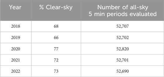
Table 2. The yearly percentage of the 5-min periods determined to be clear-sky conditions is shown. Also shown are the sample size values (N) per year from which RR and error statistics are computed. The sample sizes for greater ramp periods decrease accordingly: 10 min N/2, 15 min N/3, 30 min N/6, and 60 min N/12.

4 Results

4.1 Fleet RRs

4.1.1 RR statistics comparison

First, we evaluate the RR statistics representing stress- and worst-case scenario events (p95/p05 and p99.99/p0.01, respectively) output from ESPRR. Figure 5 shows RR statistics drawn from the entire 5-year period for the aggregated four evaluation sites, with and without the Variability Multiplier applied, compared to the observed statistics. The stress- and worst-case RRs are all less than 10% of the maximum fleet capacity per minute.

Figure 5

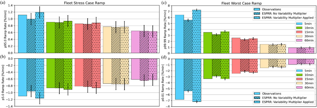
Figure 5. Ramp rate statistics p95 (A), p5 (B), p99.99 (C), and p0.01 (D) calculated using ESPRR with (spotted) and without (hatched) the variability multiplier applied are shown. The same statistics are calculated using the observations (solid) for comparison.

For the stress-case statistics, the observed percentiles fall with the confidence intervals of the ESPRR percentiles across all periods. Generally, there are minor differences in the stress-case statistics when the Variability Multiplier is applied compared to when it is not. For the worst-case statistics, however, the ESPRR percentiles with the Variability Multiplier applied correspond better to the observed percentiles than when the multiplier is not applied. This result is most evident for short-period RRs, e.g., 5–15 min. For periods 30–60 min, the ESPRR calculated RR percentiles match the observations, but there are only minor differences between having the multiplier applied or not.

Table 3 shows the RMSEs for the stress- and worst-case RR events with all periods considered. The error when using ESPRR with the Variability Multiplier applied is compared to the error without the multiplier applied using SS_RMSE (Equation 4). The SS_RMSE relative performance skill score shows a 32% improvement in error when the Variability Multiplier is applied for the stress-case events and a 48% error improvement for the worst-case RR events.

Table 3

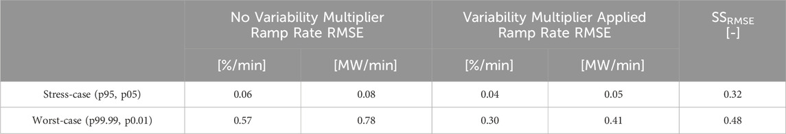
Table 3. RMSEs of stress- and worst-case RR statistics across all periods. SS_RMSE measures the RMSE performance of ESPRR (Variability Multiplier Applied) relative to the reference ESPRR (No Variability Multiplier).

4.1.2 Extreme value RR distribution comparison

Figure 5 and Table 3 evaluate ESPRR’s ability to estimate four key percentiles of the observed distribution of RRs. While the indication is that ESPRR represents the observed RRs well, we need to compare the distribution of ramp rates next. In particular, we must examine the extreme values of the distribution as this is where the Variability Multiplier is expected to have the greatest impact.

Figure 6 shows the extreme value distributions of RRs for the fleet. Values less (greater) than the distribution’s 10th (90th) percentile are shown in the histograms with gamma-fit functions drawn for both the ESPRR and the observed distribution. Across all periods, applying the Variability Multiplier acts to make the gamma function broader and flatter, meaning a distribution with a greater frequency of extreme values. For periods 10, 15, and 60 min, applying the Variability Multiplier moves the ESPRR extreme value distribution closer to the observed distribution. However, there is a trade-off; for 5- and 30-min RR periods, applying the Variability Multiplier takes the extreme value distribution to a more extreme than observed profile.

Figure 6

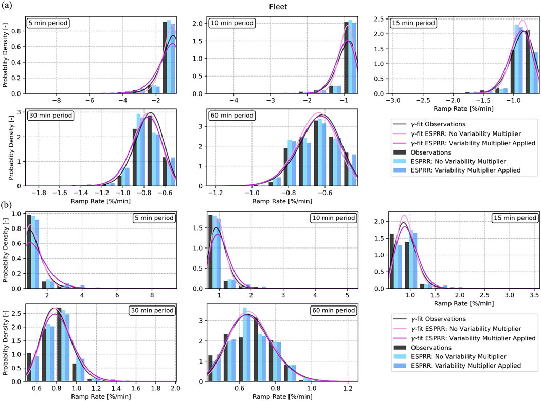
Figure 6. Extreme value probability distributions for less than the 10th percentile (A) and above the 90th percentile (B). Histograms calculated using ESPRR with (blue) and without (light blue) the variability multiplier applied are compared to observations (black). Gamma-fit functions are shown (purple, lighter purple, and grey, respectively). Each panel shows a different period for the ramp rate; 5, 10, 15, 30 and 60 min.

Overall, across the various RR periods, the net effect of applying the Variability Multiplier is an extreme value distribution closer to or fractionally exceeding observations. Ideally, we would want new PV systems and fleets to be resilient to all RRs they could face, even those not in the observed record, meaning a fractional overestimation is preferential to any underestimation. Therefore, we recommend using ESPRR with the Variability Multiplier applied for the best RR estimation.

4.2 Single-site RR evaluation

4.2.1 Yearly RR statistics

Here, we evaluate the RR statistics for a single PV system by year to highlight inter-annual variations. Figure 7 shows the worst-case RR statistics for Solar Site 1. Across the 5 years, we see consistency in observed RR percentiles for periods of 10 min and greater. However, for 5-min periods, there is a slight increase in the percentiles for 2021 and 2022. Figure 7 shows that applying the Variability Multiplier increases the ESPRR calculated percentiles, which generally better match the observed percentiles than without the multiplier. Like Figure 5, the impact of the Variability Multiplier is most evident for 5- to 15-min periods and less so for 30- to 60-min periods, where both ESPRR percentiles match the observations within confidence intervals.

Figure 7

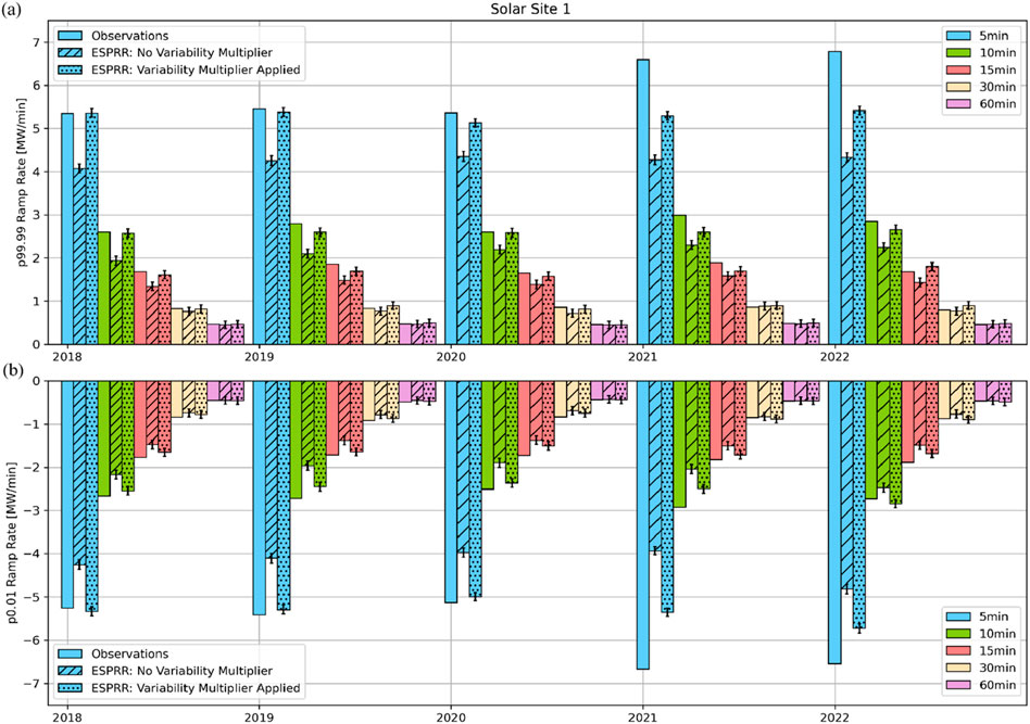
Figure 7. Ramp rate statistics p99.99 (A) and p0.01 (B) calculated for each year using ESPRR with (spotted) and without (hatched) the Variability Multiplier applied is compared to observations (solid). The period for the ramp rates is shown by the colors referenced in the legend.

4.2.2 Monthly RR statistics

Figure 8 shows the same worst-case RR statistics as Figure 7 but split by month. The worst-case scenario RR percentiles are greatest for February, March, August, and September. During February and March, the Southwest is transitioning out of the winter precipitation season, and for the 5 years studied, clear-sky percentages were 64% and 62%, respectively. With the seasonal transition bringing a greater variability of weather conditions, the intermittency of cloud conditions is expected to be greater compared to the most and least clear months (e.g., May and December). August and September are the latter part of the monsoon season, again meaning a greater variability of cloud conditions is expected.

Figure 8

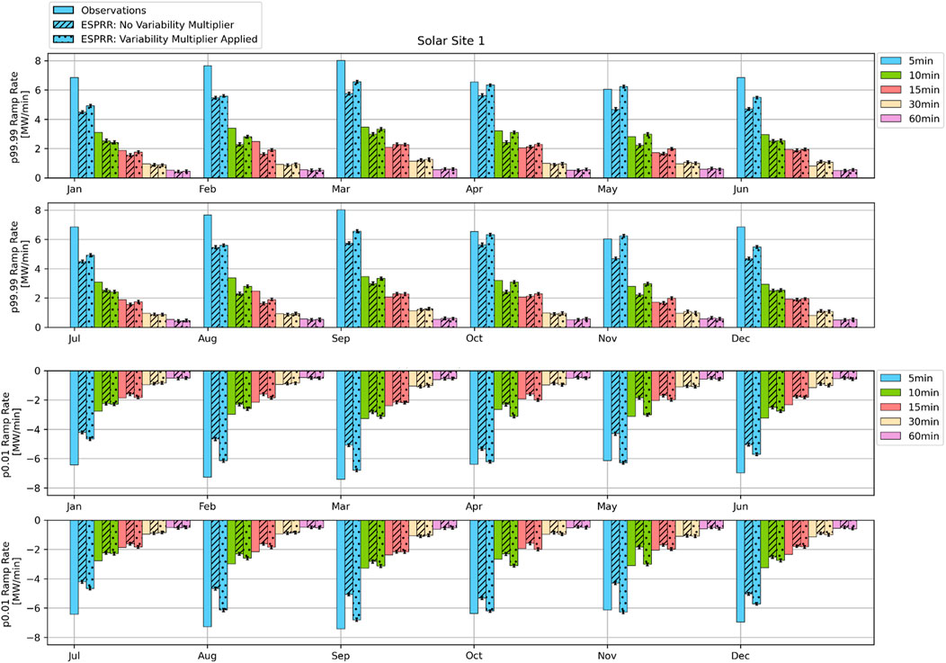
Figure 8. Ramp rate statistics p99.99 (A) and p0.01 (B) calculated for each month using all years of data. ESPRR with (spotted) and without (hatched) the Variability Multiplier applied is compared to observations (solid). The period for the ramp rates is shown by the colors referenced in the legend.

Comparing the percentiles from ESPRR with and without the multiplier applied in Figure 8 supports a similar interpretation to Figures 5, 7. ESPRR with the Variability Multiplier applied matches observations closer than without the multiplier for shorter periods (5, 10, 15 min). There is good correspondence with the observed percentiles for the longer period RRs (30, 60 min), though there are insignificant differences between the two EPSRR calculated percentiles.

4.2.3 Exceedances of worst-case RRs in observations

The number of observed RRs that exceed the ESPRR calculated monthly worst-case percentiles are shown in Supplementary Figures S2, S3 to understand the likelihood of these RR events occurring yearly. For 30-to-60-min period ramps, on average, there is less than or equal to one event that exceeds the worst-case scenario RR percentile per year. For 5-to-15-min period ramps, in some months, there can be more than one exceedance per year on average. The monthly exceedances do not follow a distinct pattern; however, winter and monsoon precipitation months generally have greater exceedances.

4.3 Fleet RRs compared to a theoretical geographically diverse fleet

To evaluate the importance of geographic diversity in minimizing fleet RRs, we create a theoretical fleet named the Geographically Diverse Fleet (GDF), which is of equal capacity to the fleet used for evaluation (136.25 MWp). Each system in the GDF is situated on the four opposing sides of Phoenix rather than the southeast side where the fleet used for evaluation is located (see Supplementary Figure S5 for map). As expected, we see lesser RRs for the GDF than the evaluation fleet, with significant differences for 5-to-15-min periods and differences within the confidence intervals for 30- to 60-min periods (see Figure 9).

Figure 9

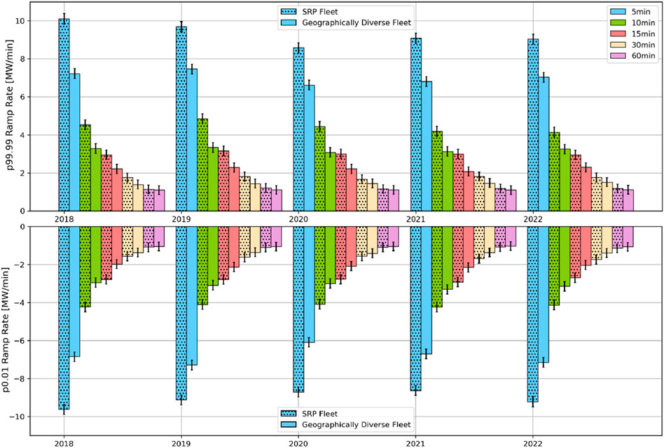
Figure 9. Ramp rate statistics p99.99 (A) and p0.01 (B) calculated for each year for the SRP fleet (spotted) versus a theoretical geographically diverse fleet (solid) using all years of data. The periods of the ramp rates are shown by the colors referenced in the legend.

4.4 Single site expected performance evaluation

Lastly, we evaluate the expected AC power time series from ESPRR at Solar Site 1. Figure 10 shows yearly error statistics, (a) NMBE and (b) NRMSE (Equations 2, 3), for clear and all-sky conditions. Figure 11 shows the same error metrics split by month. During clear-sky conditions for all years and months, the NMBE is less than 6%, and the NRMSE is 10% or less. In all-sky conditions, comparing the errors for ESPRR with and without the Variability Multiplier shows that the NMBE is reduced closer to zero when applying the multiplier. However, the RMSE increases by 1%–5% with the Variability Multiplier applied.

Figure 10

Figure 10. Normalized mean bias errors (A) and normalized root mean square errors (B) for each year of data for all-sky (blue) and clear-sky (green) conditions. Metrics for ESPRR with (solid) and without (hatched) the Variability Multiplier applied are shown and since the Variability Multiplier only operates on non-clear conditions there is only one clear-sky value.

Figure 11

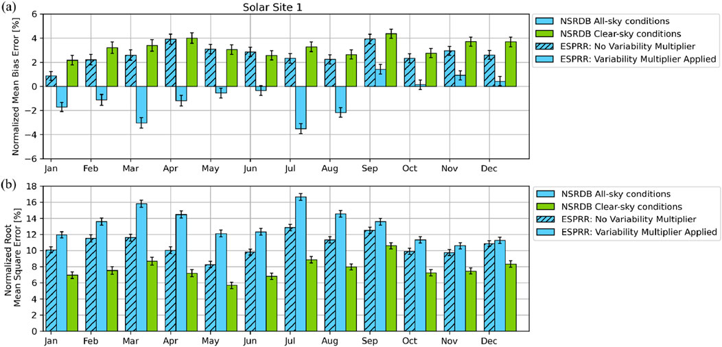
Figure 11. Normalized mean bias errors (A) and normalized root mean square errors (B) are shown for each month using all years of data for all-sky (blue) and clear-sky (green) conditions. Metrics for ESPRR with (solid) and without (hatched) the Variability Multiplier applied are shown and since the Variability Multiplier only operates on non-clear conditions there is only one clear-sky value.

5 Summary and conclusions

In this study, we describe the development of the ESPRR tool and evaluate its output expected power generation time series and ramp rate statistics. ESPRR computes an expected power generation time series using user-defined system parameters and NSRDB data input to a PV system model. Users can assess 5 years of AC power output and the characteristics of ramp rates from the proposed systems, including stress-case and worst-case RR events. The location and parameters of the proposed systems can be modified in real time to minimize RRs with no additional inputs required. Such functionality is useful when planning and designing PV systems, as it can help address growing concerns about the potential negative effects on grid reliability from the increasing penetration of utility-scale PV systems.

For the evaluation, we use generation measurements from a 136.25 MWp fleet of PV systems in Arizona from 2018 through 2022. We find that the ESPRR calculated stress-case RRs have an error of 0.05 MW/min; the error for worst-case RR events is 0.42 MW/min. We report that the frequency of exceeding the worst-case RR is less than one event per year for 30-to-60-minute RRs and less than five for 5-to-15-min RRs. We developed a time-varying multiplier to modify the power output from EPSRR on days with the greatest variability of power generation resulting from intermittent cloud conditions. The multiplier addresses features of the observed power time series that cannot be represented by the input irradiance data, like sub-grid-scale clouds or misrepresented cloud characteristics, such as optical thickness. The multiplier increases the extreme values of the distribution of RRs, particularly for 5-to-15-min ramp periods, which better matches the observed distribution. Applying the Variability Multiplier reduces the fleet-wide RR statistics error by 32% for stress-case events and 48% for worst-case RR events using all RR periods.

We evaluate the expected power generation for a single PV system and find ESPRR’s calculated AC power output in clear-sky conditions has an NRMSE of less than 10% of system capacity and an NMBE of less than 6%. In non-clear-sky conditions with the multiplier applied, the NRMSE is 10%–15% of system capacity, and the NMBE reduces to about zero. Applying the multiplier improves the statistical representation of RRs at the expense of marginally increasing the error of the AC power estimate from observations in non-clear conditions.

The Variability Multiplier is made optional so users can decide whether the better representation of RRs is the preferred selection at the expense of a 1%–5% increase in error in the expected AC power output in non-clear conditions. The expected performance error statistics presented are likely greater than we would expect in an operational forecast setting, as real-time generation information could be used to inform a persistence or bias correction model that would nudge forecasts toward recent observations and reduce error metrics. Still, such errors from the ESPRR expected power generation time series with the multiplier applied are sufficient for prospective PV system planning, as they are within the range of errors we would expect from weather forecasts used to create solar power forecasts.

Finally, we compare RR statistics from the fleet used for evaluation to statistics from a proposed fleet of equal capacity but with greater geographic diversity. From the fleet with greater geographic diversity, we find up to a 20% reduction in worst-case RR statistics for all periods, with significant differences for the 5-to-15-min RRs. This emphasizes the importance of geographic diversity when siting new PV systems, and showcases the possible magnitude of RR migitation from a sufficiently distributed fleet.

Data availability statement

The raw data supporting the conclusions of this article will be made available by the authors, without undue reservation.

Author contributions

PB: Formal Analysis, Investigation, Methodology, Project administration, Validation, Visualization, Writing–original draft, Writing–review and editing. LB: Conceptualization, Data curation, Investigation, Software, Visualization, Writing–review and editing. AL: Conceptualization, Data curation, Funding acquisition, Software, Writing–review and editing. JR: Conceptualization, Funding acquisition, Methodology, Project administration, Writing–review and editing.

Funding

The author(s) declare that financial support was received for the research, authorship, and/or publication of this article. The Salt River Project Agricultural Improvement and Power District provided the funding for this work, which supported the participation of all authors.

Acknowledgments

The authors thank William F. Holmgren for participating in early discussions and help formulating the project proposal.

Conflict of interest

Author AL was employed by Descartes Labs, Inc.

The remaining authors declare that the research was conducted in the absence of any commercial or financial relationships that could be construed as a potential conflict of interest.

Publisher’s note

All claims expressed in this article are solely those of the authors and do not necessarily represent those of their affiliated organizations, or those of the publisher, the editors and the reviewers. Any product that may be evaluated in this article, or claim that may be made by its manufacturer, is not guaranteed or endorsed by the publisher.

Supplementary material

The Supplementary Material for this article can be found online at: https://www.frontiersin.org/articles/10.3389/fenrg.2024.1434019/full#supplementary-material

References

Bolinger, M., Warner, C., and Robson, D. (2021). Utility-scale solar: empirical trends in deployment, Technology, cost, performance, PPA pricing, and value in the United States. CA, United States: Lawrence Berkeley National Laboratory, LBL Publications.

Google Scholar

Gheorghiu, C., Scripcariu, M., Tanasiev, G. N., Gheorghe, S., and Duong, M. Q. (2024). A novel methodology for developing an advanced energy-management system. Energies (Basel) 17, 1605. doi:10.3390/en17071605

CrossRef Full Text | Google Scholar

Holmgren, W. F., Hansen, C. W. W., and Mikofski, M. A. A. (2018). Pvlib Python: a Python package for modeling solar energy systems. J. Open Source Softw. 3, 884. doi:10.21105/joss.00884

CrossRef Full Text | Google Scholar

Hossain, M. K., and Ali, M. H. (2014). “Statistical analysis of ramp rates of solar Photovoltaic system connected to grid,” in 2014 IEEE energy conversion congress and exposition, ECCE 2014, 2524–2531. doi:10.1109/ECCE.2014.6953737

CrossRef Full Text | Google Scholar

Jamaly, M., Bosch, J. L., and Kleissl, J. (2013). Aggregate ramp rates of distributed photovoltaic systems in San Diego county. IEEE Trans. Sustain. Energy 4, 519–526. doi:10.1109/TSTE.2012.2201966

CrossRef Full Text | Google Scholar

Lappalainen, K., Wang, G. C., and Kleissl, J. (2020). Estimation of the largest expected photovoltaic power ramp rates. Appl. Energy 278, 115636. doi:10.1016/j.apenergy.2020.115636

CrossRef Full Text | Google Scholar

Martins, J., Spataru, S., Sera, D., Stroe, D. I., and Lashab, A. (2019). Comparative study of ramp-rate control algorithms for PV with energy storage systems. Energies 12, 1342. doi:10.3390/en12071342

CrossRef Full Text | Google Scholar

Mills, A. D., and Wiser, R. H. (2011). Implications of geographic diversity for short-term variability and predictability of solar power. IEEE Power and Energy Society General Meeting, 1–9. doi:10.1109/PES.2011.6039888

CrossRef Full Text | Google Scholar

NOAA (2023). Climate at a glance: city time series. Natl. Centers Environ. Inf. Available at: https://www.ncei.noaa.gov/access/monitoring/climate-at-a-glance/city/time-series.

Google Scholar

Sengupta, M., Xie, Y., Lopez, A., Habte, A., Maclaurin, G., and Shelby, J. (2018). The national solar radiation data base (NSRDB). Renew. Sustain. Energy Rev. 89, 51–60. doi:10.1016/j.rser.2018.03.003

CrossRef Full Text | Google Scholar

U.S. Department of Homeland Security, and Oakridge National Lab (2023). Transmission lines. Homel. Infrastruct. Foundation-Level Data. Available at: https://hifld-geoplatform.opendata.arcgis.com/.

Google Scholar

Wang, G. C., Luis Bosch, J., Kurtz, B., La Parra, I. D., Wu, E., and Kleissl, J. (2019). “Worst expected ramp rates from cloud speed measurements,” in Conference Record of the IEEE Photovoltaic Specialists Conference, 2281–2286. doi:10.1109/PVSC40753.2019.8981213

CrossRef Full Text | Google Scholar

Yang, D. (2021). Validation of the 5-min irradiance from the national solar radiation Database (NSRDB). J. Renew. Sustain. Energy 13. doi:10.1063/5.0030992

CrossRef Full Text | Google Scholar