Short-term wind power prediction and uncertainty analysis based on VDM-TCN and EM-GMM

Due to the fluctuating and intermittent nature of wind energy, its prediction is uncertain. Hence, this paper suggests a method for predicting wind power in the short term and analyzing uncertainty using the VDM-TCN approach. This method first uses Variational Mode Decomposition (VDM) to process the data, and then utilizes the temporal characteristics of Temporal Convolutional Neural Network (TCN) to learn and predict the dataset after VDM processing. Through comparative experiments, we found that VDM-TCN performs the best in short-term wind power prediction. In wind power prediction for 4-h and 24-h horizons, the RMSE errors were 1.499% and 4.4518% respectively, demonstrating the superiority of VDM-TCN. Meanwhile, the Gaussian Mixture Model (GMM) can effectively quantify the uncertainty of wind power generation at different time scales.

1 Introduction

Wind power, being the world’s most significant new energy development focus, has seen global annual new wind power installations exceeding 50 GW since 2015. In 2019 alone, the newly installed capacity increased by 19% compared to 2018, reaching 60.4 GW (GWEC, 2022). Due to its inherent characteristics, accurate prediction of wind power is essential for grid-connected operations to ensure the smooth functioning of the power grid (Zhou et al., 2023). Hence, wind power prediction holds utmost importance.

In current wind power prediction research, the prediction time scale for wind power varies due to the impact of scheduling strategies (Zhou et al., 2023). In the long-term and medium-term prediction, wind power resources are generally predicted throughout the year to target wind power siting (Desalegn et al., 2023). At the same time, the installed capacity of wind farms is configured according to the range of prediction results. In addition, the results of short-term and ultrashort-term predictions over a 3-day period are usually used for bidding for feed-in services for wind power to guarantee power quality (Hong et al., 2019), and the results of wind power predictions are used for day-ahead or intraday scheduling of the grid (Jia et al., 2024).

In the realm of wind power prediction research, the prediction technology for wind power under various scenarios is commonly categorized into physical prediction and statistical prediction (Gu et al., 2021). Physical prediction studies typically involve the joint simulation of atmospheric conditions (Zheng et al., 2022), and wind turbine behavior to forecast wind power generation over a specific time frame (Yang Y. et al., 2023). Statistical prediction techniques (Wang et al., 2024), which are typically applied to vast amounts of wind power data, utilize neural networks, multiple regression methods, and deep learning algorithms to model and predict wind power for future time periods (Meng et al., 2024).

As the depth of learning in intelligent algorithms continues to increase, the field of wind power prediction extensively employs these algorithms to develop novel prediction systems (Zhang et al., 2023). Within machine learning prediction models, temporal characteristics are commonly leveraged to assimilate historical wind power generation data (Sun and Zhao, 2020). Some researchers utilize historical and future forecast data from numerical weather predictions (NWP) to establish correlations between past inputs and outputs (Hong et al., 2019; Medina and Ajenjo, 2020). Wei et al. addressed the issue of low accuracy in ultra-short-term wind power prediction by proposing the use of LSTM for learning and prediction. They compared it with the traditional ARIMA model and found a significant improvement in prediction accuracy (Wei et al., 2023). Zhang et al. (2024) proposed a CNN-BiLSTM algorithm theory for multi-layer wind farm prediction, demonstrating a higher level of accuracy compared to traditional methods. While machine learning techniques have been widely applied in wind power prediction research, most studies have focused on their use for predictive purposes.

However, the accuracy of wind power prediction is influenced by various factors, and most individual algorithms are unable to address these challenges (Lin et al., 2024). Therefore, in recent years, hybrid algorithms have been commonly utilized in wind power prediction research (Zhu et al., 2023). For example, Yuan et al. introduced a hybrid model that combines the Least Squares Support Vector Machine (LSSVM) and the Gravitational Search Algorithm (GSA) for wind power generation prediction. They used the GSA algorithm to optimize the parameters of the LSSVM model in order to improve the prediction quality (Yuan et al., 2015). Zhou et al. (2019) proposed a K-Means-LSTM network model for wind power prediction and a bandwidth-optimised non-parametric kernel density estimation (KDE) model for probabilistic interval prediction of wind power. The K-Means clustering method is used to form different clusters of wind power impact factors to generate a new LSTM sub-prediction model. As well as non-parametric kernel density estimation generates intervals with narrower prediction intervals, higher interval coverage and higher prediction accuracy. Another study (Yuan et al., 2015) proposed a wind power prediction model based on the hybrid GWO-Copula approach to address the issue of wind power prediction distribution. It was observed that incorporating Copula with GWO (Grey Wolf optimization algorithm) significantly enhanced prediction accuracy without additional complexity. Additionally, Tu et al. developed an ARIMA-GARCH-T model to tackle the intricate timing challenges in wind power prediction, rectifying timing learning flaws and enhancing prediction accuracy (Tu et al., 2021). While the aforementioned research has made significant progress in optimizing wind power model parameters and improving model learning, there remains a limited focus on feature information processing.

In order to further enhance its ability of time series information extraction as well as anti-interference generalization, a combination of machine learning and load decomposition algorithms is often used (Zhang et al., 2018). To address the issue of poor model learning effectiveness, Deng D and colleagues developed a prediction method based on EEMD-GRU-MLR utilizing data characteristics. The Ensemble Empirical Mode Decomposition (EEMD) algorithm was employed for data decomposition, followed by evaluation of the prediction performance (Deng et al., 2020). EEMD serves as an enhanced version of Empirical Mode Decomposition (EMD). This technique necessitates the addition of white noise to the original signal to address spectral overlap, decay fluctuations, and trend information present in EMD. It filters out minor non-noise component fluctuations in the initial data, leading to irreversible loss of information. Consequently, the algorithm exhibits inherent limitations (Papazoglou et al., 2023).

Comparatively speaking, the signaling principle of the VMD algorithm is not complex, and the computational load is significantly smaller compared to EMD and EEMD. Moreover, its theoretical foundation is more robust. Unlike its predecessors, VMD does not rigidly define the meaning of each component but allows for independent selection of the number of components, enabling decomposition based on specific requirements (Kousar et al., 2022). However, new challenges have emerged with this algorithm. As each dimension of the data needs to be decomposed, predicted, and reconstructed separately, the computational time required remains substantial. To address issues related to limited algorithm accuracy, high computational complexity, lengthy model training times, low model generalization, and insufficient information extraction, this paper proposes a prediction method based on VDM-TCN for achieving high-precision wind power predictions.

Analyzing the uncertainty of wind power prediction is crucial. In uncertainty analysis methods, it can be divided into parametric methods and non-parametric methods. Parametric methods are based on point prediction models and assume the form of error distribution. However, this method may have limitations when dealing with diverse error distribution characteristics. In contrast, non-parametric methods use non-parametric estimation methods, do not need to assume the form of the target distribution, and can more accurately express the prediction error distribution, improving the analysis accuracy. For the uncertainty of wind power prediction, commonly used confidence interval methods are used for qualitative and quantitative analysis. The calculation of confidence intervals for uncertainty in wind power prediction can use parametric methods, non-parametric methods, and the decomposition and superposition of uncertainty factors. These methods help to better understand and address the uncertainty of prediction errors.

To ensure power grid stability, accurate assessment of future uncertainties in wind power bidding is crucial. While existing studies have delved into wind power prediction and uncertainty analysis, further exploration is needed to characterize multi-scale wind power prediction and uncertainty analysis. This study introduces a new wind power prediction framework based on VDM-TCN-EM-GMM to comprehensively investigate the relationship between the law and uncertainty of wind power prediction. By utilizing the VDM algorithm for data feature decomposition, the TCN algorithm for data prediction learning, and applying EM-GMM for qualitative and quantitative analysis, this study redefines the performance of wind power prediction uncertainty across multiple time scales, elucidating uncertainty patterns in wind power prediction at different time scales. The research aims to thoroughly examine uncertainties in wind power prediction, aiming to establish a robust prediction framework and provide valuable insights in this field. The process is shown in Figure 1.

(1) The key contributions of this study include the development of the comprehensive VDM-TCN-EM-GMM model, addressing challenges in quantitative wind power prediction and standardizing the process of wind power prediction uncertainty analysis. Compared to existing prediction algorithms and uncertainty analysis models, this framework can evaluate multi-time scale wind power prediction models comprehensively, enhancing the stability and accuracy of prediction results.

(2) Additionally, an in-depth investigation into prediction patterns and uncertainty characteristics across different time scales in various wind farms has been conducted, offering valuable data support and theoretical guidance for accurate wind power prediction in the future, bringing important insights for the development and application of the wind power industry.

Figure 1

Figure 1. The VDM-TCN-EM-GMM technical process.

Section 2 of this paper will introduce the principles and structures of the TCN model, the EM-based mixture Gaussian distribution model, and the confidence interval calculation model. Section 3 will present example analyses of the predictions for a wind farm using different models and time periods, along with uncertainty analysis and a comparison of the uncertainties in the confidence intervals. Finally, this study will be summarized in Section 4.

2 VDM-TCN model principle

The VDM-TCN model combines the advantages of variational mode decomposition (VDM) principles and time convolutional neural network (TCN) in a hybrid network. The VDM component decomposes the input wind power feature dataset into different modes, allowing the model to capture various fluctuation patterns present in the data. These modes are then fed into the TCN component, which utilizes temporal convolutional layers to learn the temporal dependencies and relationships of the wind power data features. The integration of VDM for mode decomposition and TCN for temporal modeling enhances the learning effectiveness of TCN, thereby improving prediction accuracy.

2.1 Principles of the TCN model

Temporal Convolutional Networks (TCNs) represent a neural network architecture specifically crafted for handling sequential data. TCNs employ one-dimensional convolutional layers to capture temporal relationships present in the input data. Through the utilization of dilated convolutions, TCNs can significantly enlarge the receptive field without a notable rise in the parameter count. This capability enables TCNs to effectively model extensive dependencies within the input sequence. Furthermore, TCNs integrate residual connections to aid in the training of deeper networks and address the issue of vanishing gradients (Yang S. et al., 2023).

In this model, the wind power feature dataset $X=\left\{x_1,x_2,x_3.....x_t\right\}$ always corresponds to the wind power generation dataset $O=\left\{o_1,o_2,o_3.....o_t\right\}$. At the same time, an intermediate hidden layer $H=\left\{h_1,h_2,h_3.....h_t\right\}$ is introduced. All outputs satisfy the causal condition restriction, i.e., the current output $y_t$ is only related to $\left\{x_1,x_2,x_3.....x_t\right\}$, and is not related to the “future” input $\left\{x_{t+1},x_{t+2},x_{t+3}.....x_{t+T}\right\}$. This is also in line with most of the time-series models in real life. This is consistent with most real-life applications, where future states are predicted with only historical data.

The relationship in the output can be represented as Eq. 1:

$o_1,o_2,o_3.....o_T=f\left(x_1,x_2,x_3.....x_T\right)(1)$

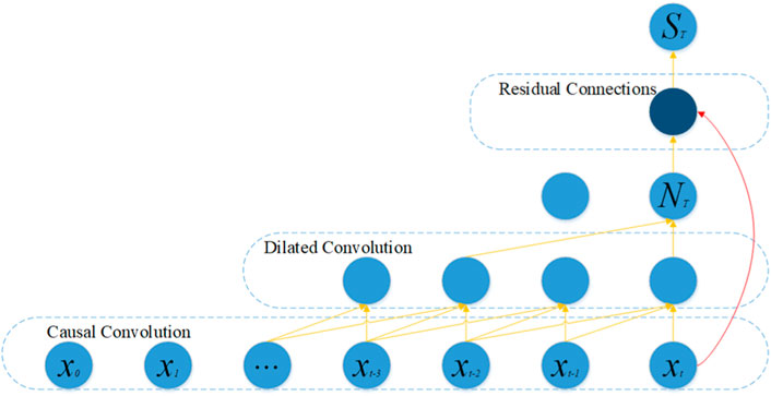
What sets TCN apart from CNN models is that it incorporates both causal convolutions and dilated convolutions. Based on the actual data types and distributions, the network architecture of TCN for wind power prediction models in this study is depicted in Figure 2. The dimension of wind power input for $\left\{x_1,x_2,x_3.....x_t\right\}$ is 10, and output for $O=\left\{o_1,o_2,o_3.....o_t\right\}$ is 1.

Figure 2

Figure 2. Structure of temporal convolutional network.

2.1.1 Causal convolutional layer

In a time convolutional neural network, a causal convolutional layer ensures that each output element depends only on past input elements, In current wind power prediction model, this primarily refers to the correspondence between the wind speed, wind direction, temperature, and other data input at time t and the wind power generation at time t. This means that the layer does not have any connections to future input elements, preventing information leakage from the future. This property is crucial for tasks where the model should not have access to future information, such as in time series prediction or sequence modeling. The hollow causal convolution used in this paper combines the temporal constraints of causal convolution with the characteristics of dilated convolution in terms of skip sampling, ensuring that the output at the current time step depends only on the preceding states and is independent of the subsequent states (Guo et al., 2023). The formula for hollow causal convolution calculation is as follows Eq. 2.

$f\left(x\right)=\left(o*f\right)x={\displaystyle \sum _{t=0}^{k-1}}f\left(i\right)X_{o-di}(2)$

Where $X$ is the input, $f$ is the filter, $d$ and $k$ are the dilation factor and convolution kernel size respectively. In the wind power prediction model based on the TCN algorithm in this study, the dataset’s dilation factor is set to 8, and the convolution kernel is set to 20.

This paper incorporates dilated convolutional layers into the constructed TCN model. The expansion convolutional layer plays a crucial role in capturing complex patterns and relationships within the temporal data by increasing the richness of the learned representations. This process enables the network to extract more intricate features and enhance its ability to learn and generalize from the input data.

2.1.2 Residual convolutional layer

Due to the large-scale data feature quantities and datasets required for wind power prediction training, using deeper networks can lead to the problem of gradient explosion. However, residual convolution can also improve the learning effectiveness of deep convolution. The residual convolutional layer in TCN (Temporal Convolutional Network) plays a crucial role in capturing long-range dependencies in sequential data. By incorporating residual connections, the network is able to learn the residual information between the input and output of each layer, allowing for easier optimization and training of deep networks. This enables the network to learn more effectively from the input data and improve the overall performance of the model. Furthermore, the residual convolutional layer in TCN allows for the efficient extraction of temporal features from sequential data by applying convolutional operations with shared weights across different time steps. This helps the network to capture complex patterns and dependencies in the data, leading to better generalization and prediction capabilities.

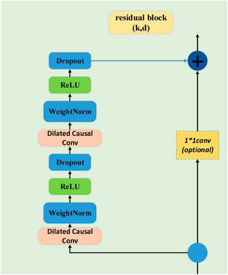
To address the channel width issue of wind power prediction data in matrices, the width of residual tensors is adjusted using 1*1 convolutions. As shown in Figure 3, in order to achieve complete coverage of the receptive field, residual blocks need to be incorporated into the TCN model. The width of the receptive field increases twofold with the addition of each residual block. Also, in order to avoid the saturation problem with multi-layer residuals, we increase the sparsity of the network by adding a corrected linear unit (ReLU) function to each layer of residuals. The calculation formula are as follows Eqs 3, 4:

$r=1+{\displaystyle \sum _{i=0}^{n-1}}2\times \left(k-1\right)\times b^i(3)$

$ReLU\left(x\right)=\mathit{max}\left(0,1\right)(4)$

Figure 3

Figure 3. Diagram of residual block.

In this context, $r$ represents the receptive field, $k$ denotes the kernel size, and $b$ stands for the dilation base.

Finally, F(X) is added to X to obtain the output value y as in Eq. 5.

$O=Activation\left(x+f\left(x\right)\right)(5)$

where $f\left(x\right)$ denotes the output of the convolutional layer and $Activation\left(.\right)$ denotes the activation function.

In terms of loss function design, this study uses the mean squared error (MSE) function to measure according to the actual characteristics of the training data as well as the specific network structure, and optimises the overall model by minimising the above error. The details are shown in Eq. 6.

$MSE=\frac{1}{N}{\displaystyle \sum _{i=1}^N}{\left(y_i-y_i^{\prime }\right)}^2(6)$

In this study, we found through experimental comparisons that RMSPropOptimizer can better ensure the stability of the error gradient of temporal convolutional neural networks during the training process, and it can modify the traditional gradient accumulation into an exponentially weighted moving average, so that it can adaptively regulate the change of the learning rate. Therefore, this study uses RMSPropOptimizer as an optimiser for TCN networks to better optimise the network model parameters. The formulas are given in Eqs 7, 8.

$Sdw=\beta Sdw-\left(1-\beta \right)d{w}^2(7)$

$W=W-\alpha \frac{dw}{\sqrt{Sdw}}(8)$

where $\beta$ is the smoothing constant, $dw$ refers to the square of the gradient and $W$ is the learnable parameter.

2.2 Variational modal decomposition

VDM (Variational Mode Decomposition) is a data-driven technique used for signal processing and analysis. It decomposes a signal into a set of modes that represent different oscillatory components of the signal. The process of VDM involves finding a set of modes that best capture the variations in the signal. This is achieved by formulating an optimization problem where the modes are obtained by minimizing a cost function that measures the differences between the original signal and its reconstructed version using the modes. The key idea behind VDM is to decompose the signal into a finite number of modes that are orthogonal to each other and capture different frequency components of the signal. This allows for a more efficient representation of the signal and can help in identifying and analyzing the underlying dynamics of the signal (Zhao et al., 2023).

Therefore, VDM needs to first use the Hilbert transform to calculate the analytic signal of each modal function $u_k\left(t\right)$, then mix the analytic signals of each mode with the central frequency $e^{-jwkt}$, and finally demodulate the signals using Gaussian smoothing and the gradient square criterion to obtain the bandwidth of each decomposition mode. The formula are as follows Eqs 9, 10:

$\min \left\{{\displaystyle \sum _{k=1}^K}‖{\beta }_t\left[\left(\beta \left(t\right)+\frac{g}{\pi t}\right){\lambda }_k\left(t\right)\right]e^{-gkwt}{\Vert }_2^2\right\}(9)$

$s.t.{\displaystyle \sum _{k=1}^K}{u}_k=f(10)$

Furthermore, the optimization is enhanced by effectively solving through the utilization of penalty function $\alpha$ and Lagrange multiplier $\beta$.

$L\left(\left\{u_k\right\},\left\{w_k\right\},\lambda \right)=\alpha {\displaystyle \sum _{k=1}^K}‖{\beta }_t\left[\left(\beta \left(t\right)+\frac{g}{\pi t}\right){\lambda }_k\left(t\right)\right]e^{-gkwt}\left|{\Vert }_2^2+‖f\left(t\right)-\left[{\lambda }_k\left(t\right)\right]\right|{\Vert }_2^2+\left[\gamma \left(t\right),f\left(t\right)-{\displaystyle \sum _{k=1}^K}{\lambda }_k\left(t\right)\right](11)$

The alternating direction multiplier method is used in VMD to solve the variational problem of Eq. 11 by alternately updating ${u_k}^{n+1}$, ${{\omega }_k}^{n+1}$, and ${{\lambda }_k}^{n+1}$ to solve the improved Lagrangian expression “saddle point”, i.e., the optimal solution of the constrained variational model in Eq. 9. where the modal components of the solution are new $u_k$ and centre frequency ${\omega }_k$, respectively:

${{\widehat{u}}_k}^{n+1}=\frac{\widehat{f}\left(\omega \right)-{\displaystyle \sum _{i\ne k}}{\widehat{u}}_i\left(\omega \right)+\frac{{\widehat{u}}_i\left(\omega \right)}{2}}{1+2\alpha \left(\omega -{\omega }_k\right)}(12)$

${\omega }_k^{n+1}=\frac{{{\int }_0^{\infty }\omega \left|\widehat{u_k}\left(\omega \right)\right|}^{2}d\omega }{{{\int }_0^{\infty }\left|\widehat{u_k}\left(\omega \right)\right|}^{2}d\omega }(13)$

2.3 EM-GMM model

As wind power prediction is affected by dataset errors as well as characterisation factors, a strong uncertainty is reflected in the prediction results, which is also known as error fluctuation. In order to ensure the competitive bidding of electricity and the stable operation of wind power, the uncertainty of wind power needs to be described to qualitatively and quantitatively analyse the prediction error of wind power to control the fluctuation range of the uncertainty error. Therefore establishing an error distribution for wind power prediction as well as establishing confidence intervals for wind power prediction is the best way to quantify the uncertainty of wind power prediction errors. The distribution models based on the combination of genetic algorithms and GMM are able to optimise these Gaussian mixture parameters using the selection, crossover and mutation operations of genetic algorithms to help the GMM fit the data distribution better. The advantage of this approach lies in its ability to fully leverage the global search capability of genetic algorithms while utilizing the flexible modeling capability of GMM, resulting in a more accurate description of the data distribution. Additionally, this combined approach can overcome the drawback of GMM being prone to local optima, thereby improving the robustness and generalization ability of the model.

2.3.1 Gaussian mixture models

GMM is a probabilistic model that represents a combination of multiple Gaussian distributions. Its structure is a method of approximating the probability distribution of a variable by linear mixing using a certain number of Gaussian functions.

Since each Gaussian component in the GMM mixture model is characterized by its mean and covariance matrix, these matrices determine the shape, position, and orientation of the distribution. At the same time, the data is generated by a mixture of Gaussian distributions under multiple weights and selections. Therefore, it is necessary to perform iterative training based on the EM algorithm, which estimates the parameters of the Gaussian components by maximizing the likelihood of the observed data, thus obtaining the optimal Gaussian parameter values. GMM is commonly used for clustering and density estimation tasks, aiming to divide the data into different groups based on the underlying distribution of the data. By using a combination of simple Gaussian components to capture the complex structure of the data, it is represented as follows Eqs 14, 15:

$P\left(X_t\right)={\displaystyle \sum _{i=1}^K}{\omega }_i\mu \left(P_t,{\gamma }_i,{\sum }_i\right)(14)$

$\mu \left(P_t,{\gamma }_i,{\sum }_i\right)=\frac{1}{{\left(2\pi \right)}^{\frac{n}{2}}{\left|{\sum }_i\right|}^{\frac{1}{2}}}\exp \left(-\frac{1}{2}{\left(P_t-{\gamma }_i\right)}^T{\sum }_i^{-1}\left(P_t-{\gamma }_i\right)\right)(15)$

where $n$ is the dimensionality of the pixel point in the high dimensional space, ${\omega }_i$ is the weight ${\displaystyle \sum _{i=1}^K}{\omega }_{i,t}=1$, ${\mu }_i$ and $m$ are the mean and covariance matrices.

The parameter estimation of GMM is generally optimised by using the algorithm of EM for nonlinear probability functions during the training process, which greatly improves the implement ability of the algorithm under the premise of guaranteeing the accuracy. The specific principle is as follows.

Assuming $x_j=\left({\omega }_j,{\mu }_j,{\sum }_j\right)$, $j=1,2,\cdots ,K$, there are a total of $K$ Gaussian models for the GMM, and all the parameters of the GMM are estimated through the sample set $X$: $\mathrm{\Theta }={\left(x_1,x_2,\cdots ,x_K\right)}^T$, then the sample $P$ is the $\log$ function with $e$ as the base in Eq. 12, i.e., it can be written as ln, but the vast majority of representations of the log-likelihood function are still expressed in Eq. 16:

$C\left(P\left|\mathrm{\Theta }\right.\right)=\log {\displaystyle \prod _{m=1}^T}{H}_K\left(P_i\right)={\displaystyle \sum _{m=1}^T}\log {\displaystyle \sum _{j=1}^R}{\omega }_j{\mu }_j\left(P_i;{\gamma }_j,{\sum }_j\right)(16)$

where T is the total number of samples, the parameters of the mixed model appropriate to the current sample set will maximise the log-likelihood function of Eq. 13, i.e., the estimation of the statistical parameters of the mixed model satisfies Eq. 17.

${\mathrm{\Theta }}_0=\arg \underset{\theta }{\max }C\left(\mathrm{\Theta }\right)(17)$

The EM algorithm is initially a statistical method that is an iterative algorithm. Assuming an initial estimate of the GMM parameters as ${\mathrm{\Theta }}^{\left(0\right)}$, and assuming that the mixed model parameters for the $q$ step iteration are ${\mathrm{\Theta }}^{\left(q\right)}$, the $q+1$ step iteration process is:

(1) Calculate the expectation (E-Step)

Calculate the posterior probability that each data belongs to the $j-th$ class of distribution according to the parameters ${\mathrm{\Theta }}^{\left(q\right)}$ of the current mixture model (Eq. 18):

${\varpi }_{ij}^{\left(q+1\right)}=\frac{{\omega }_j^{\left(q\right)}{\mu }_j\left(P_j;{\mathrm{\Theta }}^{\left(q\right)}\right)}{{\displaystyle \sum _m^K}{\omega }_r^{\left(q\right)}{\mu }_j\left(P_j;{\mathrm{\Theta }}^{\left(q\right)}\right)};1\le m\le T,1\le j\le R(18)$

(2) Maximising expectation (M-Step)

After obtaining the posterior probability that each data belongs to each subclass, Eq. 14 is solved using gradient descent to obtain an estimate of Θ at step $q+1$.

Update the weights (Eq. 19):

${\omega }_j^{\left(a+1\right)}={\displaystyle \sum _{i=1}^N}{\varpi }_{ij}^{\left(q+1\right)}(19)$

Update mean values (Eq. 20):

${\mu }_j^{\left(q+1\right)}=\frac{{\displaystyle \sum _{i=1}^N}{\varpi }_{ij}^{\left(q+1\right)}{X}_i}{{\displaystyle \sum _{i=1}^N}{\varpi }_{ij}^{\left(q+1\right)}}(20)$

Update covariance matrix (Eq. 21):

${\sum }_j^{\left(q+1\right)}=\frac{{\displaystyle \sum _{i=1}^N}{\varpi }_{ij}^{\left(q+1\right)}\left(X_i-{\mu }_j^{\left(q+1\right)}\right){\left(X_i-{\mu }_j^{\left(q+1\right)}\right)}^T}{{\displaystyle \sum _{i=1}^N}{\varpi }_{ij}^{\left(q+1\right)}}(21)$

Repeat steps (19), (20), (21) until $‖{\mathrm{\Theta }}^{\left(q+1\right)}-{\mathrm{\Theta }}^{\left(q\right)}‖$ sufficient hours to stop.

2.3.2 Confidence intervals based on GMM

Based on the use of GMM, this study incorporates confidence interval calculation to quantitatively describe the uncertainty of predictions.

The wind power prediction error is the difference between the predicted value of wind power $P_{\text{fore}}$ and the actual value of wind power $P_{\text{ture}}$ at a certain point in time, as shown in Eq. 22.

$e=P_{\text{fore}}-P_{\text{true}}(22)$

The formula is as follows:

$P\left({\alpha }_{\text{low}}<\alpha <{\alpha }_{\text{up}}\right)=1-\theta (23)$

In Eq. 23, $\left[{\alpha }_{\text{low}},{\alpha }_{\text{up}}\right]$ is the refers to the upper and lower limits of the confidence interval. $1-\theta$ is the reliability of the true value in the interval.

For uncertainty analysis modeling, it is challenging for overall error modeling or single-point error modeling to consistently demonstrate high reliability and adaptability at all times. Therefore, this study employs standard predictive analysis methods and Gaussian Mixture Model (GMM) for comprehensive analysis to enhance the clarity of predictions in uncertain scenarios.

The overall calculation steps are: Step1 Firstly, use the GMM method to establish the corresponding wind power error probability density map and calculate the wind power error probability density curve.

Step2 Under the given confidence level, find a shortest interval, so that the probability of the deterministic prediction error value falling into the interval is equal to the confidence level.

Step3 Use the (${\alpha }_{up}$ and ${\alpha }_{low}$) to derive the upper and lower limits of the wind power.

2.4 Data preprocessing techniques and predictive evaluation indicators

There are many factors affecting the prediction results in wind power prediction, among which the accuracy of the data and the size of the data volume often determine the prediction results, so it is necessary to carry out relevant preprocessing of historical data.

2.4.1 Wind power data screening

In the actual wind power generation process, due to turbine maintenance or shutdown, the power generated will be negative or zero value, as well as non-normal circumstances NWP value sudden change, such as the wind speed is greater than 40 m/s. These data in the learning and prediction process will inevitably affect the learning effect, taking into account these factors, this paper in the data preprocessing of the data to be deleted.

2.4.2 Data standardisation

In order to improve the model’s fitting results and reduce errors, the article conducted standardization processing with the following formula (Eq. 24):

$x_{norm}=\frac{x-\mathit{min}}{\mathit{max}-\mathit{min}}(24)$

Where $x_{norm}$ is the standard value of wind power; $\mathit{max}$ indicates the maximum value of wind power data; $\mathit{min}$ indicates the minimum value.

2.4.3 Evaluation index of deterministic prediction error

The root mean square error (RMSE) and mean absolute error (MAE) are used to evaluate the wind power forecast model. The formula are as follows Eqs 25–28.

$\text{RMSE}=\sqrt{\frac{1}{N}{\displaystyle \sum _{t=1}^N}{\left(P_{\text{true}}-P_{\text{fore}}\right)}^2}(25)$

$P_{\text{RMSE}}=\frac{\sqrt{\frac{1}{N}{\displaystyle \sum _{t=1}^N}{\left(P_{\text{ture}}-P_{\text{fore}}\right)}^2}}{P_{\text{cap}}}(26)$

$\text{MAE}=\frac{1}{N}{\displaystyle \sum _{t=1}^N}\left|P_{\text{true}}-P_{\text{fore}}\right|(27)$

$P_{\text{MAE}}=\frac{\frac{1}{N}{\displaystyle \sum _{t=1}^N}\left|P_{\text{true}}-P_{\text{fore}}\right|}{P_{\text{cap}}}(28)$

$P_{\text{cap}}$ is the total installed capacity of the wind farm. $P_{\text{RMSE}}$ and $P_{\text{MAE}}$ is the ratio of the RMSE and MAE to the installed capacity.

2.4.4 Error evaluation indexes of uncertainty analysis methods

The coverage rate is used to evaluate the quality of the confidence intervals, as shown in Eq. 29.

${\rho }_p=\frac{1}{m}\times {\displaystyle \sum _{i=1}^m}{\rho }_i(29)$

where ${\rho }_i$ is the coverage factor.

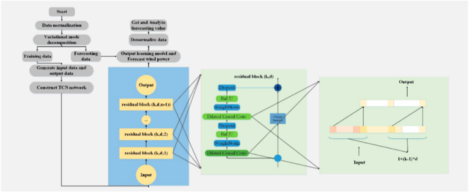
The technical route for short-term prediction and uncertainty analysis of wind power based on TCN-EM-GMM proposed in this paper is shown in Figure 4.

Figure 4

Figure 4. Wind power prediction process for VDM-TCN-EM-GMM.

3 Case study

3.1 Data sources

The wind power data originates from a wind farm located in northern China, at 114°E longitude and 41°N latitude. The wind farm has an average elevation of 1,600 m and is equipped with 90 wind turbines, each with a power capacity of 1.5 MW. The entire dataset of a wind farm with a total installed capacity of 180 MW was chosen for prediction. The rotor diameter of the wind turbines is 70.5 m, and the tower height is 67 m. The wind power prediction data used in this study includes actual output power data from the wind farm’s Supervisory Control and Data Acquisition (SCADA) system, as well as Numerical Weather Prediction (NWP) data for the wind farm. The time resolution of the actual output power data is 15 min. The NWP data is sourced from the National Meteorological Center, with a spatial resolution of 1 km. Therefore, there are multiple spatial grid points with NWP data within the wind farm, and the average of these grid points’ NWP data is used in this study. NWP data attributes include wind speed, wind direction, air pressure, temperature, and humidity, with a time resolution of 15 min. The experimental results are also in accordance with IEC standards.

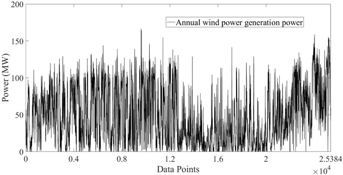
As shown in Figure 5, we selected data from the entire year of 2010 and the first half of 2011 as the study data, with a time granularity of 15 min. To evaluate the effectiveness of the algorithm, we examined data from two specific intervals (February 10–13, 2011, and August 1–3, 2011) to understand their patterns across different time scales and seasons. The input data dimension is 10, which includes 6*n decomposed data groups from VDM-decomposed wind speed, and 1*n feature data groups for wind direction, air pressure, temperature, and humidity. The output dimension is 1*n wind power generation data, where n equals the number of data points at 15-min intervals required for training and prediction.

Figure 5

Figure 5. Annual wind farm power data.

3.2 Wind power prediction and its uncertainty analysis

3.2.1 Wind power prediction analysis

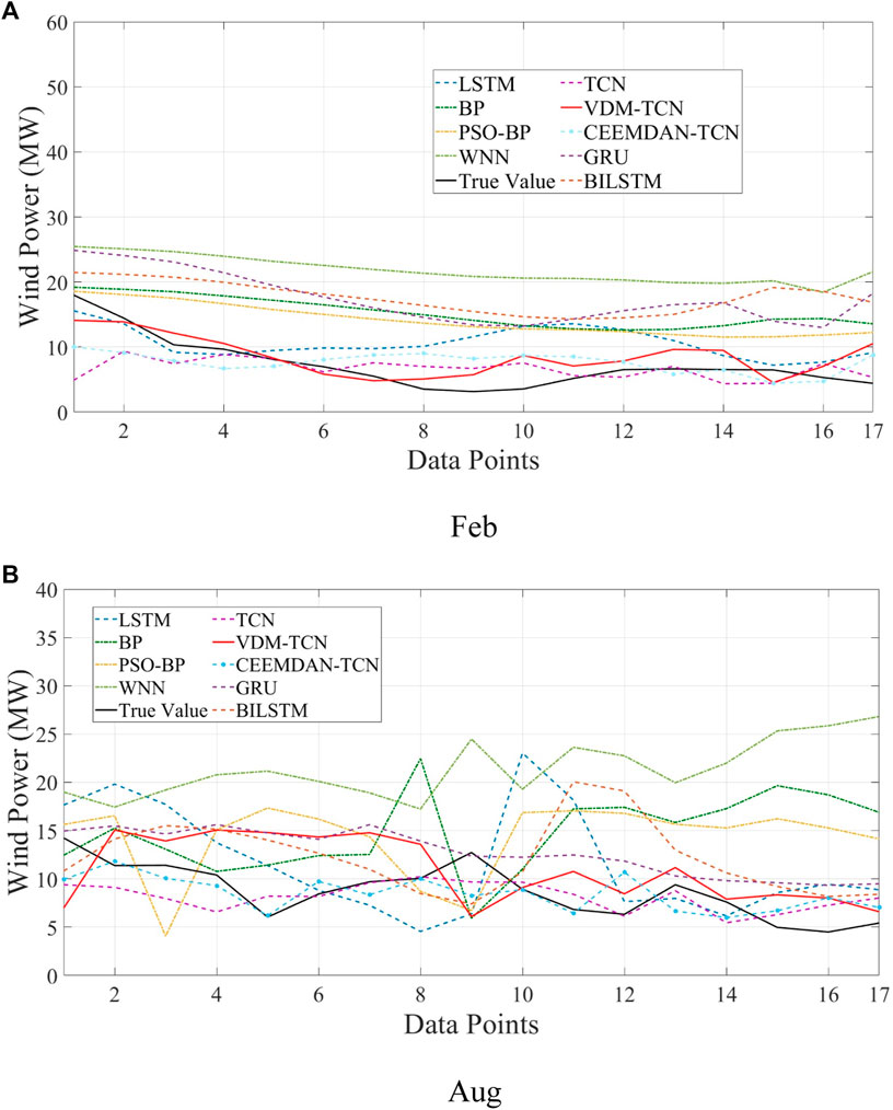
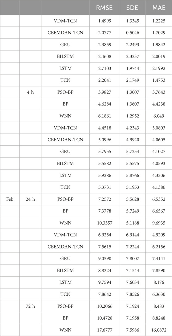
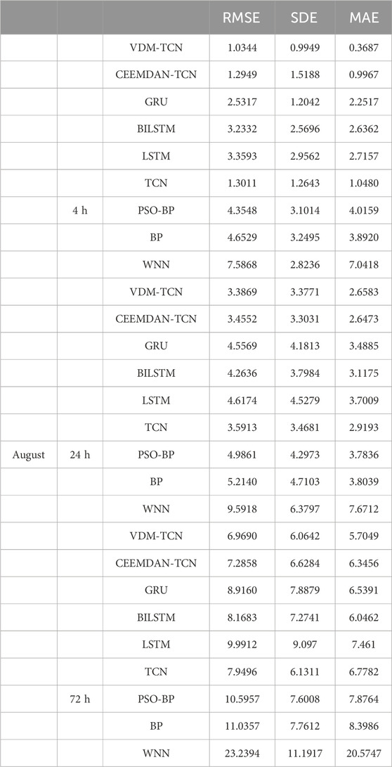
The results of wind power generation prediction for 4-h intervals on February 4th and August 3rd in winter are presented in Figures 6A, B. The red solid line represents the VDM-TCN model. It can be observed that the VDM-TCN model aligns most closely with the actual values represented by the black solid line, followed by the CEEMDAN-TCN model. Furthermore, based on the values of 4-h RMSE and MAE displayed in Table 1, it is evident that learning conducted after VDM decomposition leads to a reduction in RMSE of over 0.8% compared to learning without decomposition. Additionally, the TCN model outperforms the LSTM, BP, PSO-BP, and WNN models in the 4-h prediction. The WNN model exhibits the poorest predictive performance, yet still remains within 7%. This can be attributed to the utilization of wavelet functions in the activation function of the WNN, which results in suboptimal handling of the features of wind power data.

Figure 6

Figure 6. 4-h wind power prediction results.

Table 1

Table 1. Comparison of RMSE and MAE values for different prediction models in February.

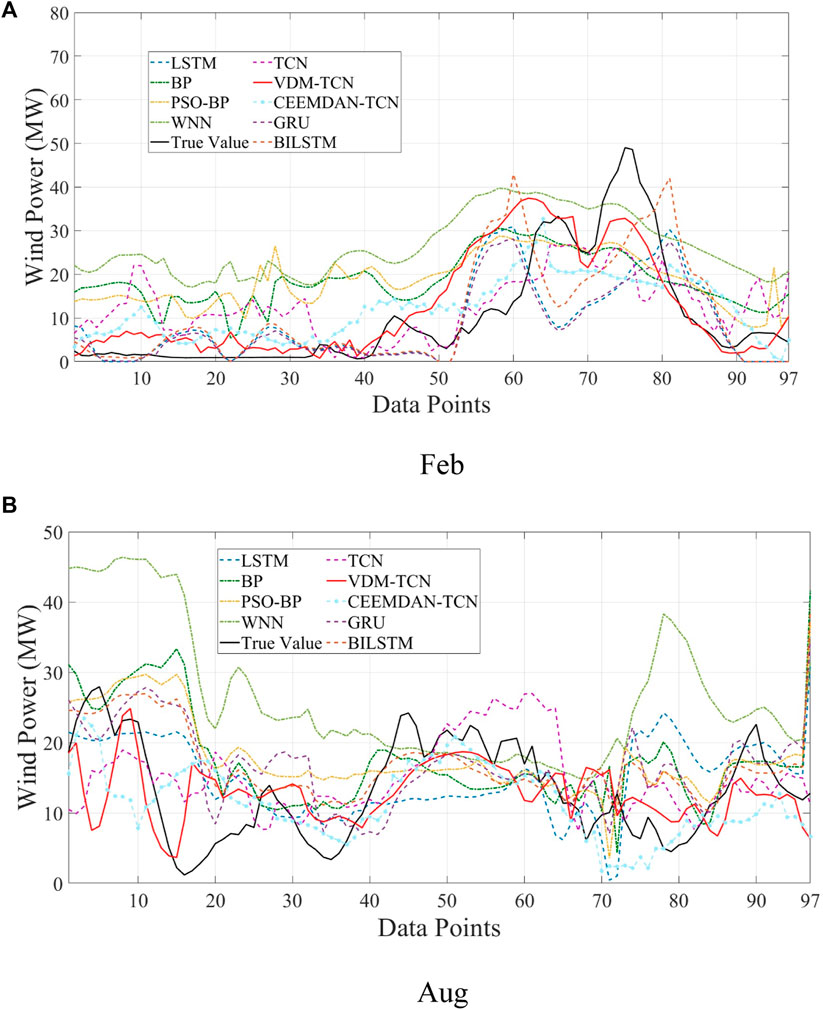
(Figures 7A, B) illustrates the 24-h wind power prediction outcomes for the 4th of February and 3rd of August during the winter season. The results indicate that VDM-TCN exhibits the highest prediction accuracy throughout the 24-h wind power prediction process. We observed a significant improvement in the prediction accuracy of the TCN algorithm after decomposing the wind power characteristic dataset, with an increase in RMSE of 0.3% compared to the undecomposed dataset. Additionally, the decomposition of the VDM algorithm exhibited higher adaptability than the CEEMDAN algorithm, showing superior predictive performance in February and August. From Figure 7A, it can be observed that, apart from VDM-TCN, the models exhibit significant discrepancies between the predicted results and the ground truth within the first 50 data points. This disparity can be attributed to the utilization of VDM for data decomposition, wherein certain anomalous frequency band data are extracted post decomposition. Consequently, the TCN model, by incorporating the anomalous characteristics of this data during the fitting process, achieves a more stable prediction outcome.

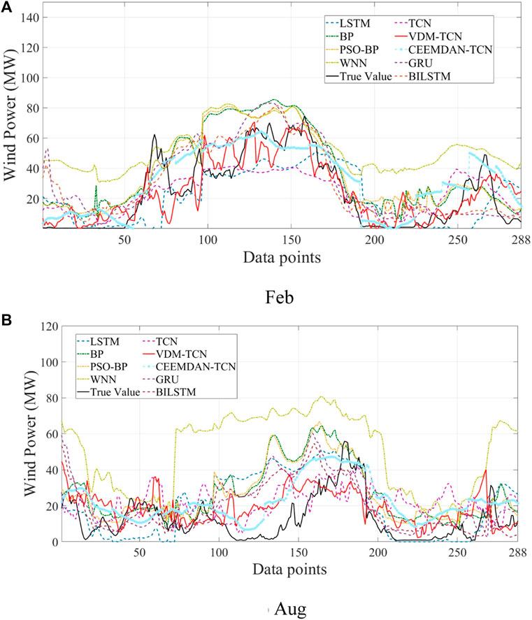
The forecast results for 72 h in Figure 8A, B show that in the 3-day forecast, VDM-TCN still maintains a significant advantage with better stability and more stable predicted values. TCN also demonstrates high predictive performance. However, data decomposed by VDM shows better learning and prediction compared to not using it. As shown in Figure 8B, although the learning and prediction effect of VDM on TCN is greatly sacrificed, some outliers still occur in small frequency bands. Through research, it was found that this is due to certain errors in the NWP values, and most importantly, the shutdown of some wind turbines in the wind farm due to wake effects and equipment damage reduces the matching degree between data and wind speed. This will also be a focus for future improvements.

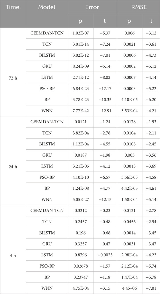
Based on the comprehensive analysis of Figures 6–8 and Tables 1, 2, it is evident that VDM-TCN demonstrates superior predictive performance across various time scales. Additionally, the TCN model exhibits high stability during predictions, thus validating the effectiveness of the VDM-TCN model in wind power prediction. These findings provide data support for subsequent uncertainty analysis, with all RMSE prediction results falling within 8%.

Figure 7

Figure 7. 24-hours wind power prediction results.

Figure 8

Figure 8. 72-h wind power prediction results.

Table 2

Table 2. Comparison of RMSE and MAE values for different prediction models in August.

The author employed a t-test to assess the significance of differences in prediction errors and RMSE results for May data from the same sample. A p-value ≤0.05 led to the rejection of the null hypothesis, indicating a significant difference in the predictive outcomes of the two models. Conversely, a p-value ≥0.05 resulted in the acceptance of the null hypothesis, suggesting no significant difference between the models’ predictions. As presented in Table 3, there were statistically significant differences between the VDM-TCN model and other models in terms of 72-h and 24-h forecasts for both prediction error and RMSE, with negative t-values, indicating that the mean prediction error and RMSE of the VDM-TCN model were lower than those of the other models, thus confirming its superior predictive performance.

Table 3

Table 3. MW level t-test distribution.

In order to better verify the accuracy and applicability of the model, we conducted ablation experiments for the VDN-TCN model with different residual convolution and number of VDM decompositions. Through Table 4, it can be clearly seen that the stability and accuracy of the prediction results are increasing with the addition of VDM and the introduction of residual convolution.

Table 4

Table 4. Comparison of RMSE results for VDN-TCN models with different residual convolution and number of VDM decompositions.

3.2.2 Wind power forecast and quantitative distribution analysis

Although the prediction errors of wind power generation can be qualitatively analyzed, it is still challenging to quantify them. In order to characterize the distribution of prediction errors in wind power generation quantitatively, this study utilizes GMM estimation to establish confidence intervals.

To calculate the confidence intervals for wind power generation prediction, the computation of probability density distribution is first required. In this study, a mixture of Gaussian model (GMM) and non-parametric kernel density estimation method are employed to obtain the probability density distribution of wind power prediction errors. Figures 9, 10 illustrate the probability distributions of wind power generation forecast errors for 72 h and 24 h. It can be observed that the non-parametric kernel density estimation method is more accurate than GMM in capturing trends across a wide range of distributions, but falls short in capturing certain abrupt changes at small scales compared to GMM. This discrepancy arises from the non-parametric kernel density estimation method’s use of smoothing kernel functions to fit observed data points for modeling the true probability distribution curve, which is susceptible to bandwidth and data influences.

Figure 9

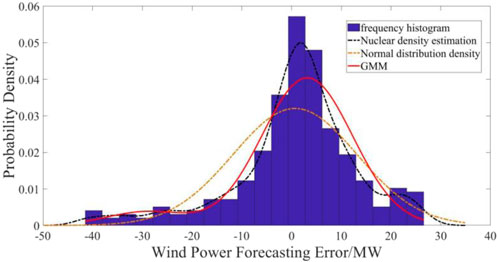
Figure 9. The 72-h probability density distribution of wind power prediction error under different distribution models.

Figure 10

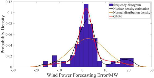
Figure 10. The 24-h probability density distribution of wind power prediction error under different distribution models.

In order to better demonstrate the superiority of the GMM algorithm, we chose non-parametric kernel density estimation (NPKDE) and Gaussian modelling (GM) to contrast with the GMM algorithm and compare the uncertainty ranges of the predictions of different algorithms.

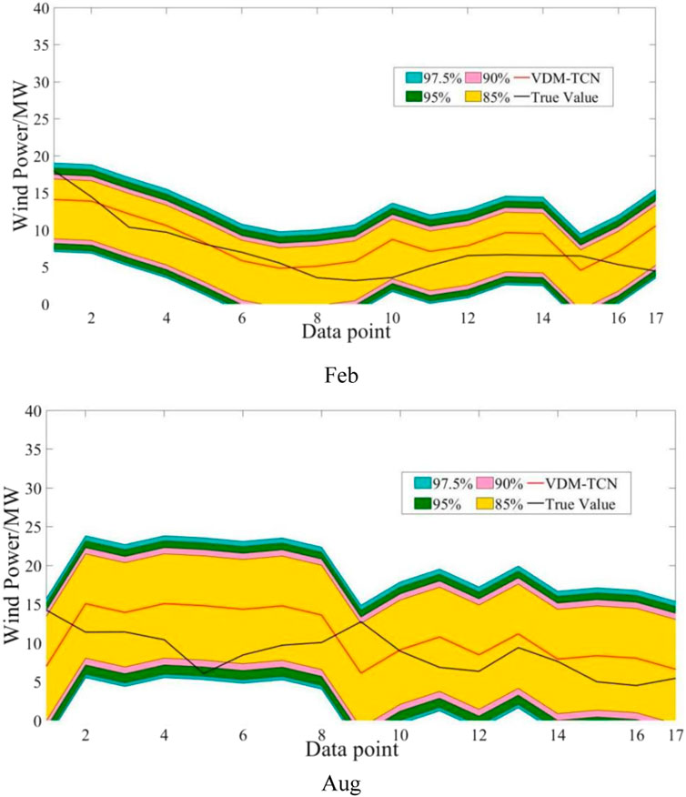
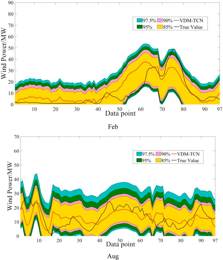
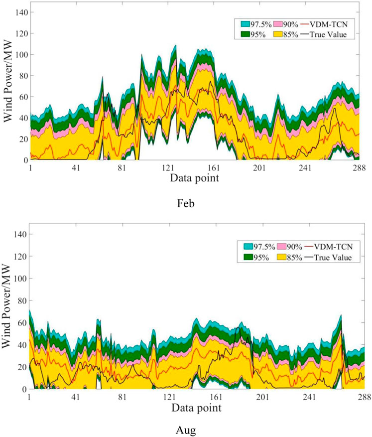
From the data, it can be observed that for Figures 11–13, the probability of the prediction values for the entire wind energy decreases with confidence intervals greater than the current confidence level. However, some forecasted values are not included in the confidence intervals due to actual output power changes caused by NWP errors, changes in operating states or gusts, and other factors. Furthermore, as the confidence level increases, the width of the confidence interval also increases, with a higher probability of encompassing the forecasted values, which aligns with the principles of confidence interval calculations.

Figure 11

Figure 11. Distribution of confidence intervals for the 4-h prediction of the VDM-TCN model.

Figure 12

Figure 12. Distribution of confidence intervals for the 24-h prediction of the VDM-TCN model.

Figure 13

Figure 13. Distribution of confidence intervals for the 72-h prediction of the VDM-TCN model.

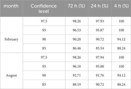
As shown in Table 5, we observe that the prediction intervals of the VDM-TCN model have high coverage rates at different confidence levels. Additionally, the VDM-TCN demonstrates high stability across various time ranges. Its coverage area meets the basic requirements of including the true values. This also proves that the GMM algorithm can accurately quantify the requirements of wind power prediction uncertainty.

Table 5

Table 5. Coverage rate of confidence interval for wind power based on VDM-TCN model.

4 Conclusion

This study innovatively proposes a method for short-term wind power prediction and uncertainty analysis using the VDM-TCN-GMM approach, which facilitates multi-scale short-term predictions of wind power via the VDM-TCN model. By applying variational mode decomposition technology to decompose the NWP, this method enhances feature diversity and improves data assimilation. Furthermore, the TCN model is utilized to identify and extract relationships among sequential features, thereby facilitating learning within a time-series framework. The Gaussian mixture model is also used to qualitatively analysis the uncertainty of wind power prediction and establish confidence intervals for quantitative analysis, and the following conclusions are drawn:

(1) The proposed VDM-TCN model not only has a temporal recursive nature, but also has an obvious advantage in feature extraction learning, which makes the VDM-TCN model have an obvious advantage in predicting wind power with time series characteristics.

(2) The prediction errors of the VDM-TCN model are all within 8%, with an improvement in RMSE prediction performance of over 1%.

(3) GMM is able to quantitatively calculate the distribution range and quantitative analysis of the prediction uncertainty in wind power generation. The coverage of the confidence interval is larger than the confidence level in 4 h, 24 h, and 72 h wind power prediction.

Although we have carried out multi-scale prediction and uncertainty analysis of wind power using VDM-TCN and EM-GMM algorithms, there is still a large amount of work that needs to be carried out for further research, and some of the much-needed work is as follows: 1) Wind power prediction needs to be further explored in terms of the impact of multi-source feature datasets on wind power prediction. 2) More algorithms need to be introduced into the field of wind power prediction to demonstrate the prediction performance of different models in different environments. 3) In terms of wind power uncertainty analysis, wind power uncertainty models will be further developed in the future to provide more accurate qualitative and quantitative analyses of wind power prediction.

Data availability statement

The original contributions presented in the study are included in the article/Supplementary Material, further inquiries can be directed to the corresponding author.

Author contributions

BP: Conceptualization, Data curation, Formal Analysis, Methodology, Validation, Writing–original draft, Writing–review and editing. JZ: Data curation, Investigation, Project administration, Supervision, Writing–review and editing. YL: Project administration, Resources, Supervision, Writing–original draft. XG: Conceptualization, Data curation, Funding acquisition, Resources, Writing–review and editing. JH: Data curation, Investigation, Writing–review and editing. RL: Visualization, Writing–review and editing.

Funding

The author(s) declare that financial support was received for the research, authorship, and/or publication of this article. Science and Technology Project of China Southern Power Grid Co., Ltd (No. 030000KC23040062 (GDKJXM20230367)).

Acknowledgments

We thank China Southern Power Grid Corporation Limited for providing financial and data support.

Conflict of interest

Authors BP, JZ, YL, XG, JH, and RL were employed by Guangdong Power Grid Co., Ltd.

The authors declare that this study received funding from the Science and Technology Project of China Southern Power Grid Co., Ltd. The funder had the following involvement in the study: manuscript preparation, data collection and analysis, and publication decisions.

Publisher’s note

All claims expressed in this article are solely those of the authors and do not necessarily represent those of their affiliated organizations, or those of the publisher, the editors and the reviewers. Any product that may be evaluated in this article, or claim that may be made by its manufacturer, is not guaranteed or endorsed by the publisher.

Supplementary material

The Supplementary Material for this article can be found online at: https://www.frontiersin.org/articles/10.3389/fenrg.2024.1404165/full#supplementary-material

References

Deng, D., Li, J., Zhang, Z., Teng, Y., and Huang, Q. (2020). Short-term electric load forecasting based on EEMD-GRU-MLR. PST 44, 593–602. doi:10.13335/j.1000-3673.pst.2019.0113

CrossRef Full Text | Google Scholar

Desalegn, B., Gebeyehu, D., Tamrat, B., and Tadiwose, T. (2023). Wind energy-harvesting technologies and recent research progresses in wind farm control models. Front. Energy Res. 11. doi:10.3389/fenrg.2023.1124203

CrossRef Full Text | Google Scholar

Gu, B., Zhang, T., Meng, H., and Zhang, J. (2021). Short-term forecasting and uncertainty analysis of wind power based on long short-term memory, cloud model and non-parametric kernel density estimation. Renew. Energy. 164, 687–708. doi:10.1016/j.renene.2020.09.087

CrossRef Full Text | Google Scholar

Guo, G., Yuan, W., Liu, J., Lv, Y., and Liu, W. (2023). Traffic forecasting via dilated temporal convolution with peak-sensitive loss. IEEE Intell. Transp. Syst. Mag. 15, 48–57. doi:10.1109/mits.2021.3119869

CrossRef Full Text | Google Scholar

GWEC (2022). Global wind report 2022. Brussels, Belgium: GWEC Europe Office.

Google Scholar

Hong, D. Y., Ji, T. Y., Li, M. S., and Wu, Q. H. (2019). Ultra-short-term forecast of wind speed and wind power based on morphological high frequency filter and double similarity search algorithm. Int. J. Electr. Power Energy Syst. 104, 868–879. doi:10.1016/j.ijepes.2018.07.061

CrossRef Full Text | Google Scholar

Jia, J., Zhang, G., Zhou, X., Shi, Z., Zhu, M., and Lv, X. (2024). Research on joint dispatch of wind, solar, hydro, and thermal power based on pumped storage power stations. Front. Energy Res. 12. doi:10.3389/fenrg.2024.1373588

CrossRef Full Text | Google Scholar

Kousar, S., Zafar, N. A., Ali, T., Alkhammash, E. H., and Hadjouni, M. (2022). Formal modeling of IoT-based distribution management system for smart grids. Sustainability 14, 4499. doi:10.3390/su14084499

CrossRef Full Text | Google Scholar

Lin, Q., Cai, H., Liu, H., Li, X., and Xiao, H. (2024). A novel ultra-short-term wind power prediction model jointly driven by multiple algorithm optimization and adaptive selection. Energy 288, 129724. doi:10.1016/j.energy.2023.129724

CrossRef Full Text | Google Scholar

Medina, S. V., and Ajenjo, U. P. (2020). Performance improvement of artificial neural network model in short-term forecasting of wind farm power output. J. Mod. Power Syst. Clean. Energy. 8, 484–490. doi:10.35833/mpce.2018.000792

CrossRef Full Text | Google Scholar

Meng, A., Zhang, H., Dai, Z., Xian, Z., Xiao, L., Rong, J., et al. (2024). An adaptive distribution-matched recurrent network for wind power prediction using time-series distribution period division. Energy 299, 131383. doi:10.1016/j.energy.2024.131383

CrossRef Full Text | Google Scholar

Papazoglou, E. L. L., Karmiris-Obratanski, P., Karkalos, N. E. E., Thangaraj, M., and Markopoulos, A. P. P. (2023). Theoretical and experimental analysis of plasma radius expansion model in EDM: a comprehensive study. Int. J. Adv. Manuf. Technol. 126, 2429–2444. doi:10.1007/s00170-023-11292-6

CrossRef Full Text | Google Scholar

Sun, Z., and Zhao, M. (2020). Short-term wind power forecasting based on VMD decomposition, ConvLSTM networks and error analysis. Ieee Access 8, 134422–134434. doi:10.1109/access.2020.3011060

CrossRef Full Text | Google Scholar

Tu, Q., Miao, S., Yao, F., Li, Y., Yin, H., Han, J., et al. (2021). Forecasting scenario generation for multiple wind farms considering time-series characteristics and spatial-temporal correlation. J. Mod. Power Syst. Clean. Energy. 9, 837–848. doi:10.35833/mpce.2020.000935

CrossRef Full Text | Google Scholar

Wang, Y., Zhao, K., Hao, Y., and Yao, Y. (2024). Short-term wind power prediction using a novel model based on butterfly optimization algorithm-variational mode decomposition-long short-term memory. Appl. Energy. 366, 123313. doi:10.1016/j.apenergy.2024.123313

CrossRef Full Text | Google Scholar

Wei, J., Wu, X., Yang, T., and Jiao, R. (2023). Ultra-short-term forecasting of wind power based on multi-task learning and LSTM. Int. J. Electr. Power Energy Syst. 149, 109073. doi:10.1016/j.ijepes.2023.109073

CrossRef Full Text | Google Scholar

Yang, S., Moreira, J., and Li, Z. (2023a). Bioinspired encoder-decoder recurrent neural network with attention for hydroprocessing unit modeling. Ind. Eng. Chem. Res. 62, 18526–18540. doi:10.1021/acs.iecr.3c01953

CrossRef Full Text | Google Scholar

Yang, Y., Liu, J., Yang, Y., Xiao, J., and Alkhateeb, A. F. (2023b). An efficient hybrid method to predict wind speed based on linear regression and VMD. Fractals 31. doi:10.1142/s0218348x23401357

CrossRef Full Text | Google Scholar

Yuan, X., Chen, C., Yuan, Y., Huang, Y., and Tan, Q. (2015). Short-term wind power prediction based on LSSVM-GSA model. Energy Convers. manage. 101, 393–401. doi:10.1016/j.enconman.2015.05.065

CrossRef Full Text | Google Scholar

Zhang, J., Wei, Y.-M., Li, D., Tan, Z., and Zhou, J. (2018). Short term electricity load forecasting using a hybrid model. Energy 158, 774–781. doi:10.1016/j.energy.2018.06.012

CrossRef Full Text | Google Scholar

Zhang, T., Huang, Y., Liao, H., Gong, X., and Peng, B. (2024). Short-term power forecasting and uncertainty analysis of wind farm at multiple time scales. Ieee Access 12, 25129–25145. doi:10.1109/access.2024.3365493

CrossRef Full Text | Google Scholar

Zhang, T., Huang, Y., Liao, H., and Liang, Y. (2023). A hybrid electric vehicle load classification and forecasting approach based on GBDT algorithm and temporal convolutional network. Appl. Energy. 351, 121768. doi:10.1016/j.apenergy.2023.121768

CrossRef Full Text | Google Scholar

Zhao, H., Zhang, H., Su, G., and Shi, X. (2023). Defect diagnosis method of cable shielding layer based on frequency domain reflection coefficient spectrum. IEEE Trans. Electromagn. Compat. 65, 114–125. doi:10.1109/temc.2022.3213351

CrossRef Full Text | Google Scholar

Zheng, C., Yi, C., Shen, C., Yu, D., Wang, X., Wang, Y., et al. (2022). A positive climatic trend in the global offshore wind power. Front. Energy Res. 10. doi:10.3389/fenrg.2022.867642

CrossRef Full Text | Google Scholar

Zhou, B., Ma, X., Luo, Y., and Yang, D. (2019). Wind power prediction based on LSTM networks and nonparametric kernel density estimation. Ieee Access 7, 165279–165292. doi:10.1109/access.2019.2952555

CrossRef Full Text | Google Scholar

Zhou, K., Han, H., Li, J., Wang, Y., Tang, W., Han, F., et al. (2023). Interval model of a wind turbine power curve. Front. Energy Res. 11. doi:10.3389/fenrg.2023.1305612

CrossRef Full Text | Google Scholar

Zhu, J., He, Y., and Gao, Z. (2023). Wind power interval and point prediction model using neural network based multi-objective optimization. Energy 283, 129079. doi:10.1016/j.energy.2023.129079

CrossRef Full Text | Google Scholar