Adaptive SPP–CNN–LSTM–ATT wind farm cluster short-term power prediction model based on transitional weather classification

With the expansion of the scale of wind power integration, the safe operation of the grid is challenged. At present, the research mainly focuses on the prediction of a single wind farm, lacking coordinated control of the cluster, and there is a large prediction error in transitional weather. In view of the above problems, this study proposes an adaptive wind farm cluster prediction model based on transitional weather classification, aiming to improve the prediction accuracy of the cluster under transitional weather conditions. First, the reference wind farm is selected, and then the improved snake algorithm is used to optimize the extreme gradient boosting tree (CBAMSO-XGB) to divide the transitional weather, and the sensitive meteorological factors under typical transitional weather conditions are optimized. A convolutional neural network (CNN) with a multi-layer spatial pyramid pooling (SPP) structure is utilized to extract variable dimensional features. Finally, the attention (ATT) mechanism is used to redistribute the weight of the long and short term memory (LSTM) network output to obtain the predicted value, and the cluster wind power prediction value is obtained by upscaling it. The results show that the classification accuracy of the CBAMSO-XGB algorithm in the transitional weather of the two test periods is 99.5833% and 95.4167%, respectively, which is higher than the snake optimization (SO) before the improvement and the other two algorithms; compared to the CNN–LSTM model, the mean absolute error (MAE) of the adaptive prediction model is decreased by approximately 42.49%–72.91% under various transitional weather conditions. The relative root mean square error (RMSE) of the cluster is lower than that of each reference wind farm and the prediction method without upscaling. The results show that the method proposed in this paper effectively improves the prediction accuracy of wind farm clusters during transitional weather.

1 Introduction

Under the background of the transformation of a global energy structure to low carbon and the continuous optimization of an energy consumption structure, China has formulated a dual-carbon plan of carbon peak and carbon neutralization, and the demand for renewable energy continues to grow. Wind energy has become one of the most widely developed and applied renewable energy sources due to its outstanding advantages such as abundant resources, environmental protection, high automation of operation and management, and continuous reduction of electricity costs. However, wind power has strong intermittence and volatility. When wind power is connected to the grid on a large scale, it will have a serious impact on the stable operation of the power grid and power quality. Transitional weather is the weather that has undergone major changes, such as typhoons and cold waves. During this period, the sudden change in wind speed and temperature will even lead to the damage of the unit equipment and the occurrence of large-scale off-grid blackouts. Therefore, accurate wind power prediction helps assist the steady-state operation of the power system, rationally allocate energy storage, and reduce operating costs.

The current wind power prediction methods are mainly divided into three categories. The first category is the physical model based on numerical weather prediction (NWP) which includes features such as wind direction, pressure, temperature, and roughness to simulate the wind power. This method requires a large amount of historical meteorological data, the calculation is very complex, and the accuracy of the model is greatly affected by the accuracy of weather forecast. The second category is statistical and probabilistic models, such as moving average model, autoregressive integrated moving average (ARIMA) model, and Bayesian model. They focus on the time-varying relationship of time series and establish a mapping relationship between predicted power and historical data based on historical output data; however, the strong nonlinearity of wind power is difficult to solve using the statistical method, especially when there are obvious errors in dealing with wind sequences with large oscillations. Therefore, the third category, machine learning model and hybrid model, has become the focus of the current research. The machine learning method considers the nonlinear relationship between the output and multiple input features and has high prediction accuracy and generalization ability. The machine learning methods include LSTM, back propagation neural network (BPNN), and extreme learning machine (ELM). Xiong et al. (2022) proposed a secondary optimization RMSprop–SFLA–BP model, which uses the RMSprop algorithm with a stronger purpose to perform a secondary gradient descent on the objective function to obtain better initial values of BPNN hyperparameters. Liu et al. (2021) proposed a new combined loss function to update BPNN to build the wind power prediction model. Gong et al. (2022) first decomposed the wind power data via EMD to eliminate the non-stationary sequence and then used the MA-BP model for prediction. However, BPNN is a gradient descent method, which is sensitive to the initial parameter values and often converges to the local optimal solution. Even if the meta-heuristic algorithm is used to optimize BPNN, it often obtains high-quality inferior solutions, and it has low training efficiency for high-dimensional data and insufficient generalization performance.

Compared to BPNN, support vector machine (SVM) tends to perform better in short-term wind power prediction duet to its advantages of fitting high-dimensional nonlinear data. Wang et al. (2020) divided the historical data into multiple clusters according to different features of different periods to establish their own prediction models and achieved good performance and computational efficiency in different scenarios. Zhang et al. (2017) used the least square support vector machine model with error correction to improve prediction accuracy. To overcome the problem of selecting SVM kernel function, Yue et al. (2020) used the whale optimization algorithm (WOA) to optimize the parameters, and Huang et al. (2022) used the grid search method to optimize the kernel function and penalty factor of SVM, which improved the prediction accuracy of the model. However, the efficiency of SVM in dealing with large sample data is relatively low, and the conventional SVM only supports binary classification. When solving multi-classification problems, model combinations are needed to solve them, and the complexity of the model is not conducive to engineering implementation.

As a special recurrent neural network (RNN) with the input gate, output gate, and forget gate, LSTM can memorize long-term temporal features and enhance the processing ability of long sequences. Shahram et al. (2022) used the hyperparameter optimization framework Optuna to optimize the hyperparameters of LSTM. Wang et al. (2023) also proposed an improved sparrow search algorithm (SSA) to optimize the parameters. Mohamad et al. (2023) proposed a new coati optimization algorithm to optimize the parameters of the CNN–LSTM hybrid model, and the prediction accuracy and persistence of these models have been improved. Fu et al. (2018) proved the superiority of LSTM compared with SVM and other methods. Liu and Zhang (2022) introduced a sparse pooling (SP) structure into the CNN–LSTM model to process data with different resolutions. Liu et al. (2023) proposed an LSTM network structure combining multiple graph convolution network (GCN) to deal with high-dimensional input and achieved good prediction performance.

The meteorological data show a certain degree of inertia in space, and it changes gradually between the adjacent locations, that is, the state information of a wind farm will affect the state information of other wind farms nearby. However, the current research on wind power prediction is mainly focused on the prediction of a single wind turbine or wind farm, and the various models established only utilize the data of time dimension, which has some limitations. Extending the power prediction of a single wind turbine or wind farm to the wind farm cluster and introducing the information of spatial dimension can further improve the upper limit of prediction accuracy.

In addition, it is mostly aimed at the overall power prediction for a period of time at present. On the one hand, the prediction of the whole wind farm cluster can coordinate the resource allocation of wind farms in the region according to the prediction results. On the other hand, there is a potential spatial correlation between adjacent wind farms. This spatial correlation is shown on the time scale, which represents the influence of wind information of the current reference wind farm on the surrounding wind farm at the next moment. Fully considering this correlation can further improve the prediction accuracy in the transitional weather period, facilitate the timely exchange of information among wind farms in the region, coordinate the adjustment of unit power generation plans, reduce abandoned wind power, and improve economic benefits (Ye and Zhao, 2014; Peng et al., 2016; Xue et al., 2017). Yang et al. (2021) divided the cluster into time series clusters based on the difference in NWP in time series and finally predicted the power of the entire wind farm cluster. Zhang et al. (2021) predicted the standard wind farm and then upscaled it to characterize the power of the entire wind farm cluster. According to the performance index of each wind farm in the cluster, Ye et al. (2018) designed a rolling optimization of the physical–statistical combined prediction model; however, the prediction accuracy of the transitional weather was still insufficient. Yu et al. (2022) modeled the probability density of transitional weather prediction errors, which improved the forecast performance to a certain extent.

1.1 Contribution and novelty of the study

In view of the lack of detailed analysis of the impact factors of transitional weather in the current prediction scheme mentioned above, the problem of ignoring time continuity caused by selecting different characteristics for different transitional weather and establishing their own prediction models, and the problem of focusing on the power prediction of a single wind farm without analyzing the whole wind farm cluster, this paper proposes an adaptive prediction model of the wind farm cluster based on transitional weather classification to improve the power prediction accuracy of transitional weather. First, the reference wind farm in the cluster is selected, and the snake algorithm based on chaotic initial population and dynamic adjustment of mutation step size theory is used to optimize the parameters of XGB to construct the transitional weather classification model. According to the classification results, different input features under different weather conditions are selected, and then a convolutional neural network (CNN) with three-layer spatial pyramid pooling (SPP) is constructed to fully extract the input features of different dimensions. The obtained fixed dimension results are input into the long- and short-term memory (LSTM) network, and the output of the long- and short-term memory network is re-weighted by the attention (ATT) module before the final fully connected layer so as to realize the wind power prediction under transitional weather. The prediction results of each reference wind farm are upscaled to obtain the final cluster prediction results.

The main contributions of this study are as follows:

(1) Accurate transitional weather classification results are helpful in selecting the optimal input features and improving the prediction effect of the model. The improved snake optimization algorithm proposed in this paper can effectively improve the classification accuracy of the XGB model for various transitional weather conditions.

(2) The sensitive meteorological factors in various transitional weather periods are analyzed and selected in detail, which are used as the input of the model to avoid the negative influence of low correlation factors.

(3) Different transitional weather has different sensitive features. In order to make the model fully extract the features of various dimensions and avoid the destruction of time continuity caused by modeling transitional weather separately, the three-layer SPP structure is designed at the CNN layer. This enables the model to fully extract sequence features while maintaining the continuity of time.

(4) The transitional weather is a short-term process in the whole time series. The important features of the short-term process are easily ignored. In this paper, the ATT mechanism is added to the LSTM layer to avoid the problem of ignoring the key features in the short-term transitional weather.

2 Basic work

Due to the inertia of meteorological factors, they gradually change in the vicinity of adjacent locations. For a wind farm cluster, the meteorological and power data between adjacent wind farms are likely to have high correlation, and the data provided for the cluster prediction are also very similar. If all wind farms in the cluster are predicted and fitted separately, it will provide too much redundant information to the model, and the high dimensionality of the data will cause overfitting, leading to a decrease in the generalization ability and prediction accuracy of the model. Therefore, it is necessary to select a reference wind farm in the wind farm cluster that contains the most valuable information as the basis for the upscaling prediction of the wind farm cluster.

2.1 Reference wind farm selection

Pearson’s correlation coefficient formula is shown in Eq. 1:

${\rho }_{x,y}=\frac{{\displaystyle \sum _{t=1}^N}\left(p_{x,t}-{\overline{p}}_{x,t}\right)\left(p_{y,t}-{\overline{p}}_{y,t}\right)}{\sqrt{{\displaystyle \sum _{t=1}^N}{\left(p_{x,t}-{\overline{p}}_{x,t}\right)}^2}\sqrt{{\displaystyle \sum _{t=1}^N}{\left(p_{y,t}-{\overline{p}}_{y,t}\right)}^2}}.(1)$

Table 1 illustrates the corresponding relationship between the range of Pearson’s correlation coefficient and the correlation strength of variables.

TABLE 1

TABLE 1. Correlation coefficient and correlation strength relationship table.

In Eq. 1,$p_{x,t}$ and $p_{y,t}$ are the power measurement values of wind farm x and cluster y at time point t, respectively, or the power measurement values of any two wind farms at time point t, and N is the length of the time series.

The scale of the wind power cluster is generally large, and there are many wind farms inside. Therefore, the wind farms with a high correlation coefficient are clustered and divided into multiple sub-clusters. Then, the correlation between individual output and overall output is analyzed in each sub-cluster, and the best reference wind farm is selected for each sub-cluster (Wang et al., 2017). The final selected multiple reference wind farms contribute the most to the features of the cluster with little redundant data.

2.2 Upscaling model

For cluster power prediction, one method is to analyze the historical power data of the cluster point. It is similar to the prediction of a single wind farm, and the cluster prediction value is obtained by mining the time series change rule. This method considers a single factor and has relatively large limitations. The other method is used to map the power of the cluster through upscaling, which first analyzes the data information in the cluster to obtain the best reference wind farm that can represent the features of the cluster and then maps the power prediction value of the cluster through the power of the wind farm in a certain proportional relationship.

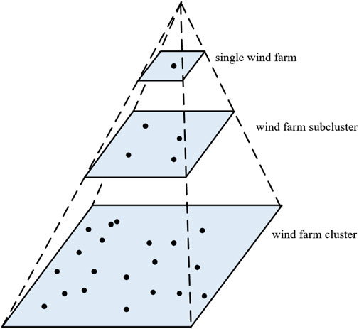
However, for large-scale wind farm clusters, it is difficult to find a special reference wind farm, called the standard wind farm, that can map the cluster power well. Therefore, the direct mapping method from the single reference wind farm to the cluster is greatly affected by the prediction accuracy of the reference wind farm, and there must be great volatility. However, by dividing sub-clusters, multiple mapping can better represent cluster power. Specifically, this is an indirect mapping method. First, the entire wind farm cluster is divided into multiple sub-clusters. The power of the corresponding sub-cluster is obtained by mapping the power of the reference wind farm in the sub-cluster, and then the power of the entire wind farm cluster is obtained by mapping the power of these sub-clusters. The upscaling model is shown in Figure 1. The predicted value $P_{G,i}$ of the cluster power at time i calculated using the upscaling model can be obtained by Eqs 2, 3:

$P_{G,i}={\displaystyle \sum _{n=1}^E}{a}_n{P}_{n,i},(2)$

$a_n=\frac{C_e}{C_n}.(3)$

FIGURE 1

FIGURE 1. Upscaling model.

Here, E is the number of sub-clusters of wind farm clustering. Each wind farm sub-cluster has a reference wind farm. The weight coefficient of the reference wind farm n is $a_n$, the installed capacity is $C_n$, the installed capacity of the corresponding sub-cluster is $C_e$, and the power prediction value of the reference wind farm n at time i is $P_{n,i}$.

2.3 Transitional weather

In addition to the necessary shutdown of wind turbines in order to ensure safety in extreme weather, the transitional weather that has a great impact on the operation of wind turbines is mainly divided into high wind speed fluctuation weather, low-temperature icing weather, high-temperature weather, and heavy precipitation weather (Zeng and Chen, 2019). Wind speed begins to increase from a certain minimum threshold and reaches the maximum threshold after a series of fluctuations. Again, it drops to reach the minimum threshold. This time period is called a high wind speed fluctuation process. In the high wind speed fluctuation weather, wind speed is the most significant feature. In the low-temperature icing weather, the wind turbine blade is partially iced, which will lead to uneven mass distribution and increased load. It is difficult to achieve rated power when the wind speed is not high. At this time, in addition to wind speed, the features of temperature and relative humidity should be considered to improve prediction accuracy. Wind power generation has the features of low wind speed at high temperature. During the high-temperature period, air density is often low and wind power is small. In addition, the high temperature will overload the internal line of the wind turbine, further limiting the power of the operation. The impact of heavy precipitation on wind power is more complicated. On the one hand, heavy precipitation weather will increase air density and change atmospheric circulation, thus affecting wind speed. On the other hand, the angle of rain hitting the wind turbine blade and the uneven quality caused by water on the blade surface will also affect power generation.

In this paper, four types of transitional weather, namely, low-temperature icing weather, high-temperature weather, heavy precipitation weather, and high wind speed fluctuation weather, are selected. Their labels are 1, 2, 3, and 5, respectively, and the labels of the other types of weather are 4. Among them, the high wind speed fluctuation weather, according to the wind speed sequence and the actual conditions of each wind farm, has the normalized wind speed of 0.3 selected as the minimum threshold and 0.6 selected as the peak threshold. In this interval, the period of time that meets the conditions of high wind speed fluctuation can be determined as a high wind speed fluctuation process.

3 The establishment of the SPP–CNN–LSTM–ATT network based on transitional weather classification

3.1 Weather classification model based on the improved SO-XGB algorithm

3.1.1 XGB

As an improved version of GBDT, XGB uses an incremental approach. The new tree generated by each iteration will fit the residual of the previous tree, fix the error of the previous tree classification, and use gradient lifting to continuously reduce the loss of the previously generated decision tree with parallel processing capabilities. The final classification prediction results are obtained by summing multiple decision trees. The calculation formulas are shown in Eqs 4, 5:

${\widehat{y}}_i={\displaystyle \sum _{a=1}^A}{f}_a\left(x_i\right),(4)$

$x_i=\left[x_{i,1},x_{i,2},L,x_{i,m}\right].(5)$

Here, ${\widehat{y}}_i$ is the classification category corresponding to the feature set $x_i$ of sample i, and $x_i$ has m features. $f_k\left(x_i\right)$ represents the weight of sample i classified to the leaf node in the tree a, and the number of trees is A. The calculation formula of the objective function $L_{obj}$ of the decision tree is shown in Eq. 6:

$L_{obj}={\displaystyle \sum _{i=1}^n}l\left({\widehat{y}}_i,y_i\right)+{\displaystyle \sum _{k=1}^K}\mathrm{\Omega }\left(f_k\right).(6)$

Here, ${\displaystyle {\sum }_{i=1}^n}l\left({\widehat{y}}_i,y_i\right)$ is the loss function, which is used to measure the difference between the predicted category ${\widehat{y}}_i$ and the actual category $y_i$, and the objective function is approached using the second-order Taylor expansion (Li and Liu, 2019), which not only increases accuracy but also facilitates the custom loss function (Su et al., 2023). The advantage of the XGB tree is that the regularization term ${\displaystyle {\sum }_{k=1}^K}\mathrm{\Omega }\left(f_k\right)$ is introduced to punish the complex model and prevent overfitting (Zhao et al., 2019). The calculation formula is shown in Eq. 7:

$\mathrm{\Omega }\left(f_k\right)=\gamma T+\frac{\lambda }{2}{\displaystyle \sum _{j=1}^T}{\omega }_j^2.(7)$

Here, $\gamma$ and $\lambda$ are regularization coefficients, which are used to control the number of leaf nodes T and the weight ${\omega }_j$ of the leaf node j.

3.1.2 A snake optimization algorithm combining Bernoulli chaotic map and bidirectional adaptive Cauchy mutation (CBAMSO)

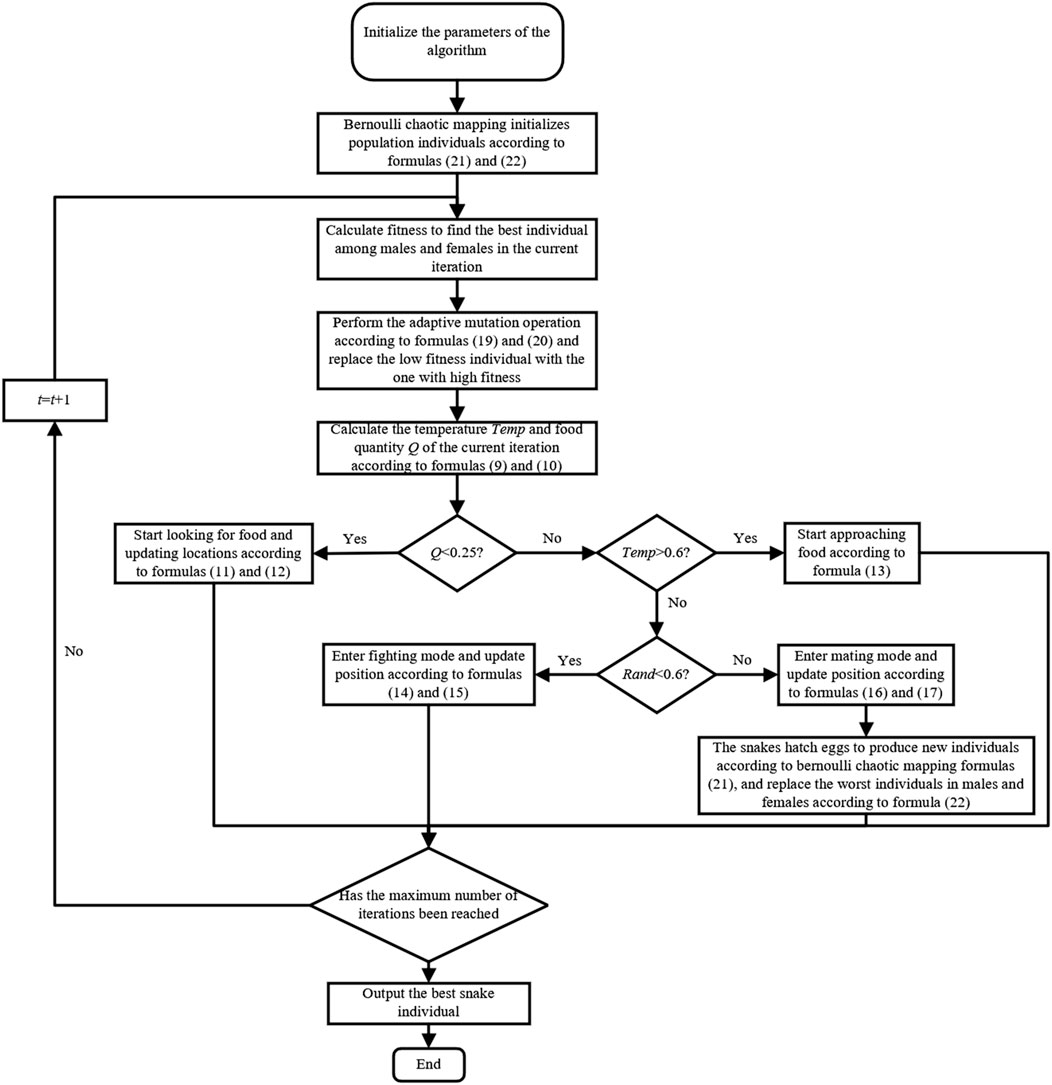
The snake optimization algorithm is inspired by the snake‘s foraging and breeding behavior (Hashim and Hussien, 2022). Affected by temperature Temp and food quantity Q at the same time, the snake group can be divided into three behavioral patterns: food search mode, fighting mode, and mating mode.

First, an initial population $x_i$ is generated. The total number of individuals in the population is n, in which males and females are equally divided. The initialization formula is shown in Eq. 8:

$x_i=x_{\mathit{min}}+r\times \left(x_{\mathit{max}}-x_{\mathit{min}}\right).(8)$

The temperature formula is shown in Eq. 9:

$Temp\left(t\right)=\mathit{exp}\left(\frac{-t}{T}\right).(9)$

The food quantity formula is shown in Eq. 10:

$Q\left(t\right)=c_1\times \mathit{exp}\left(\frac{t-T}{T}\right).(10)$

When Q < 0.25, the snake group chooses a random location to search for food and updates the location. The location update formulas for males and females are shown in Eqs 11, 12, respectively:

$x_i^{m/f}\left(t+1\right)=x_r^{m/f}\left(t\right)\pm c_2\times A_{m/f}\times \left(\left(x_{\mathit{max}}-x_{\mathit{min}}\right)\times r+x_{\mathit{min}}\right),(11)$

$A_{m/f}=\mathit{exp}\left(\frac{-f_r^{m/f}}{f_i^{m/f}}\right).(12)$

When Q > 0.25 and Temp > 0.6, the snake group begins to approach food, and the population position update formula is shown in Eq. 13:

$x_i^{m/f}\left(t+\right)=x_{food}\left(t\right)\pm c_3\times Temp\left(t\right)\times r\times \left(x_{food}\left(t\right)-x_i^{m/f}\left(t\right)\right).(13)$

When Q > 0.25 and Temp < 0.6, a random value is generated. If it is less than the threshold of 0.6, the snake group will enter the fighting mode. The male and female position update formulas are shown in Eqs 14, 15, respectively:

$x_i^{m/f}\left(t+1\right)=x_i^{m/f}\left(t\right)+c_3\times F_{m/f}\times r\times \left(Q\left(t\right)\times x_{best}^{f/m}\left(t\right)-x_i^{m/f}\left(t\right)\right),(14)$

$F_{m/f}=\mathit{exp}\left(\frac{-f_{best}^{f/m}}{f_i^{m/f}}\right).(15)$

Otherwise, the snake group enters the mating mode, and the male and female position update formulas are shown in Eqs 16, 17, respectively:

$x_i^{m/f}\left(t+1\right)=x_i^{m/f}\left(t\right)+c_3\times M_{m/f}\times r\times \left(Q\left(t\right)\times x_i^{f/m}\left(t\right)-x_i^{m/f}\left(t\right)\right),(16)$

$M_{m/f}=\mathit{exp}\left(\frac{-f_i^{f/m}}{f_i^{m/f}}\right).(17)$

After mating, snakes can choose whether to hatch eggs. If they choose to hatch, the worst male and female individuals will be replaced. The replacement formula is shown in Eq. 18:

$x_{worst}^{m/f}=x_{\mathit{min}}+r\times \left(x_{\mathit{max}}-x_{\mathit{min}}\right).(18)$

The snake optimization algorithm uses multiple fixed parameters $c_1$, $c_2$, and $c_3$, which is easy to cause local convergence. The mutation operation can jump out of the local optimum to a certain extent, but the size of the mutation step has a great influence on the optimal solution. If the step size is too small, the generated mutation individual shows little difference from the original individual and cannot jump out of the convergence region. If the step size is too large, it may destroy the structure of the original individual, generate an invalid sample, reduce computational efficiency, and affect model performance. Therefore, this paper proposes a bidirectional adaptive Cauchy mutation strategy to add perturbations to the optimal solution and worst solution of each iteration at the same time. By comparing the fitness of the mutation individual and the original individual in the current iteration, the step size of the individual variation in the next iteration is dynamically adjusted so as to improve the problem that the algorithm is easy to fall into the local optimal solution and improve the effect of population evolution and convergence speed. The bidirectional adaptive Cauchy mutation operation update formula is shown in Eq. 19:

${\widehat{x}}_{best/worst}^{m/f}\left(t+1\right)=x_{best/worst}^{m/f}\left(t\right)+x_{best/worst}^{m/f}\left(t\right)\times {\phi }_{best/worst}\left(t\right)\times Cauthy\left(\mathrm{0,1}\right).(19)$

The calculation formula of the adjustment factor ${\phi }_{best/worst}$ is shown in Eq. 20:

${\phi }_{best/worst}\left(t\right)=\left|{\widehat{f}}_{best/worst}^{m/f}\left(t\right)-f_{best/worst}^{m/f}\left(t\right)\right|.(20)$

Here, $Cauthy\left(\mathrm{0,1}\right)$ represents the function of generating standard Cauchy random variables. Comparing the fitness of the position before and after the mutation, if the fitness is higher after the mutation, the position before the mutation is replaced; otherwise, the original position is retained.

When the population is generated and the snake hatches eggs to reset the worst solution, a pseudo-random number with non-uniform distribution is used. The chaotic sequence has orbital instability and is highly dependent on the initial value. Even if the two similar initial values are iterated, a completely different sequence of random numbers will be obtained. Therefore, this paper uses the Bernoulli chaotic map instead of pseudo-random number initialization to expand the search area, increase the diversity of the population, and improve global search performance. The formula of Bernoulli chaotic map is shown in Eq. 21:

${\text{z}}_{\text{k}+1}=\left\{\begin{array}{l}\frac{{\text{z}}_{\text{k}}}{1-\lambda },{\text{z}}_{\text{k}}\in \left[\mathrm{0,1}-\lambda \right],\\ \frac{{\text{z}}_{\text{k}}-1+\lambda }{\lambda },{\text{z}}_{\text{k}}\in \left.\left(1-\lambda ,1\right.\right].\end{array}\right.(21)$

Here, $z_{k+1}$ represents the chaotic sequence generated by k iterations, and the value of $\lambda$ is 0.6.

The formula of Bernoulli chaotic map initialization is shown in Eq. 22:

${\widehat{x}}_i^{m/f}=x_{\mathit{min}}+z_{k+1}\times \left(x_{\mathit{max}}-x_{\mathit{min}}\right).(22)$

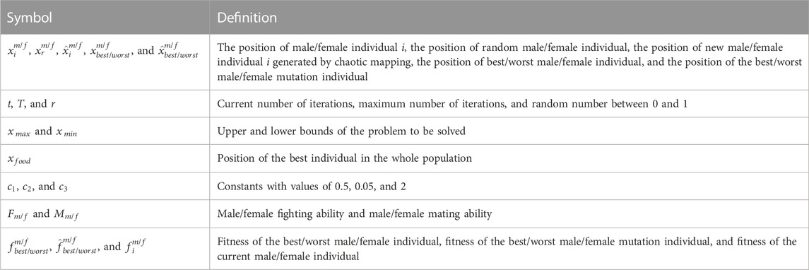
The specific flowchart of the CBAMSO algorithm is shown in Figure 2. The improved snake optimization algorithm is used to optimize the learning rate, tree depth, and optimal number of XGB trees with the error rate of sample classification as the objective function. The parameters mentioned in the above algorithm and their definitions are shown in Table 2.

FIGURE 2

FIGURE 2. Flowchart of the CBAMSO algorithm.

TABLE 2

TABLE 2. Parameter definition of the snake optimization algorithm.

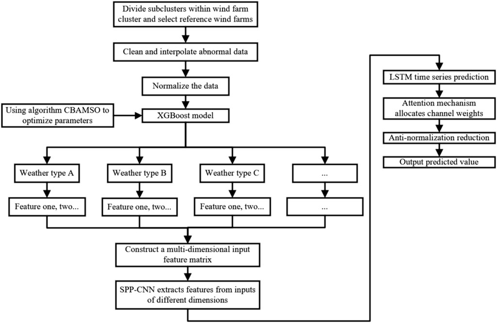
Based on the above XGB model and the improved snake optimization algorithm, the steps of the transitional weather classification task are as follows, which is also shown in the first half of the flowchart of the complete method used in this paper shown in Figure 6.

(1) Mark the weather types of the sample data manually, and select a certain number of weather types to train the model.

(2) Initialize the XGB tree, and obtain the optimal hyperparameters through the improved snake optimization algorithm.

(3) Use the NWP data and the corresponding marked weather type as the input and output, respectively, to train the XGB model.

(4) Input the test set to verify the accuracy of the model classification.

(5) Introduce NWP data from the validation set into the trained model to classify weather types.

3.2 Prediction model based on SPP–CNN–LSTM–ATT

3.2.1 SPP–CNN

CNN is a type of deep feedforward neural network with local connection and weight sharing. It has strong feature extraction ability and is widely used in computer vision, natural language processing, and other fields.

After optimizing the features, the input feature dimension of the time series samples is constantly changing. Traditional truncation or filling to make the input feature dimension consistent will inevitably cause high-dimensional input samples to lose a large amount of effective data, and low-dimensional input samples fill up a large amount of invalid information, resulting in low feature extraction effects. If LSTM prediction models are established for input samples with different features, the time continuity of meteorological data is ignored and the requirements of the LSTM model are not met. Therefore, this paper introduces a special spatial pyramid pooling structure to realize the feature extraction of variable length input by CNN without adding or deleting sample data while ensuring the time continuity of data.

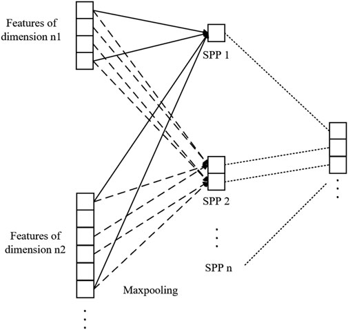
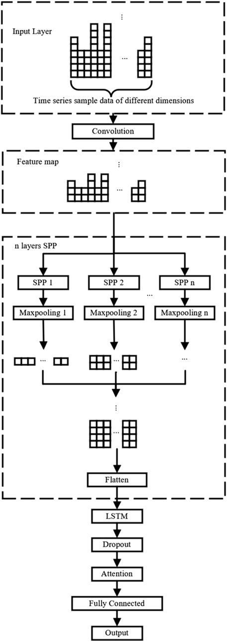
Spatial pyramid pooling processes the input feature dimension by fixing the pooling output dimension. According to the fixed pooling output dimension n, the input features are divided into n parts, and the maximum pooling is performed in each region. The granularity of a single spatial pyramid pooling layer is too coarse to fully extract the features of different dimension inputs, which will lead to insufficient model training and low performance. In this paper, a multilayer spatial pyramid pooling structure is used to splice the pooling results of each layer and transfer them to the flattening layer to fully extract the features of inputs of different dimensions. The multi-layer spatial pyramid pooling process of features of different dimensions is shown in Figure 3.

FIGURE 3

FIGURE 3. Multi-layer spatial pyramid pooling process of features of different dimensions.

3.2.2 LSTM

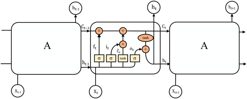
LSTM is a special recurrent neural network that is often used to deal with time axis problems. It can solve long-term dependence and gradient disappearance or explosion problems in general recurrent neural networks (Kim and Byun, 2022). Each unit of LSTM comprises four function layers, and the information transmission is controlled by the forget gate, memory gate, and output gate structures. The structure of LSTM is shown in Figure 4.

FIGURE 4

FIGURE 4. Structure of LSTM.

Each A represents an LSTM unit. When the data pass through LSTM, it will first pass through the forget gate, which will read the output $h_{t-1}$ of the previous moment and the input $x_t$ of the current moment. Through the sigmoid neural layer and point-by-point multiplication operation, each number in the unit state $c_{t-1}$ is given a number between 0 and 1, which represents the weight of whether to let the information pass. Then, the memory gate passes through two steps: the tanh function layer first extracts the effective information in the current vector and then uses the sigmoid function to control how much these memories should be put into the unit state to complete the screening of effective information. Finally, the output gate will first use the sigmoid function to extract the effective information in the vector integrated by the current input value and the previous output value. The tanh function will compress and map the unit state to the interval (−1,1) and then multiply the sigmoid function and tanh function to obtain the output of LSTM at time t.

The calculation formulas mentioned above are shown in Eqs 23–28:

$f_t=sigmod\left(W_f\cdot \left[h_{t-1},x_t\right]+b_f\right),(23)$

$i_t=sigmod\left(W_i\cdot \left[h_{t-1},x_t\right]+b_i\right),(24)$

${\stackrel{\sim }{c}}_t=\mathit{tanh}\left(W_c\cdot \left[h_{t-1},x_t\right]+b_c\right),(25)$

$o_t=sigmod\left(W_o\cdot \left[h_{t-1},x_t\right]+b_o\right),(26)$

$h_t=o_t\cdot \mathit{tanh}\left(c_t\right),(27)$

$c_t=f_t\cdot c_{t-1}+i_t\cdot {\stackrel{\sim }{c}}_t.(28)$

Here, $W_f$, $W_i$, $W_c$, and $W_o$ represent the weight matrices for the forget gate, memory gate, intermediate output, and output gate, respectively. Meanwhile, $b_f$, $b_i$, $b_c$, and $b_o$ represent the constant parameter matrices for the forget gate, memory gate, intermediate output, and output gate, respectively.

3.2.3 Attention mechanism

Attention mechanism is a deep learning method that simulates human visual attention, and its essence is a resource redistribution strategy. When LSTM processes the input sequence, each hidden layer is given the same weight. Transitional weather is a short-term change process in the whole time series. Therefore, the key features in this short-term process are easily discarded as invalid information, which leads to the insufficient learning effect of the model on transitional weather. The attention mechanism calculates the attention weight by comparing the correlation between the previous hidden layer vector and the output, improves the extraction of effective information, realizes the dynamic extraction of key parts in the time series, and ensures that the model fully learns the key features of the transitional weather period.

First, the LSTM hidden layer output $H_t$ is used as the input of the attention layer to train the weight coefficient $S_t$ through the fully connected layer. The calculation formula is shown in Eq. 29:

$S_t=\mathit{tanh}\left(\omega H_t+b_t\right).(29)$

The weighted sum of the weight coefficient and the hidden layer output is used to obtain the output result $o_t$. The calculation formula is shown in Eq. 30:

$o_t={\displaystyle \sum _{t=1}^N}{S}_t{H}_t.(30)$

3.2.4 Adaptive prediction model

During the transitional weather period, meteorological factors, such as temperature, air pressure, and wind speed, change greatly, which have a great impact on the prediction results. At this time, the influence of sensitive meteorological factors on power will be magnified, and the influence of other factors on power will be reduced. If all the features are fully considered, meteorological factors with lower correlation will have a negative impact on power prediction results. Therefore, after optimizing the features based on the CBAMSO-XGB weather classification model, it is coupled with SPP–CNN–LSTM–ATT, and different features are selected according to different weather scenarios to construct an adaptive prediction model, which can improve the prediction accuracy under transitional weather conditions. The structure of the proposed SPP–CNN–LSTM–ATT combined model network is shown in Figure 5, and the complete flowchart of the CBAMSO-XGB–SPP–CNN–LSTM–ATT adaptive prediction model is shown in Figure 6.

FIGURE 5

FIGURE 5. Structure of the SPP–CNN–LSTM–ATT combined model network.

FIGURE 6

FIGURE 6. Flowchart of the CBAMSO-XGB–SPP–CNN–LSTM–ATT adaptive prediction model.

4 Case analysis and discussion

4.1 Dividing into sub-clusters and selecting their respective reference wind farms

The example selects a wind farm cluster in northern China, which comprises seven wind farms. The installed capacity of each wind farm is shown in Table 3. The data source comprises a total of 35,136 sets of NWP and power data from seven wind farms in 2020. The time resolution is 15 min, and the features are wind speed and directions at 10 m, 30 m, 50 m, and 70 m, temperature, relative humidity, air pressure, and power.

TABLE 3

TABLE 3. Installed capacity of each wind farm in the cluster.

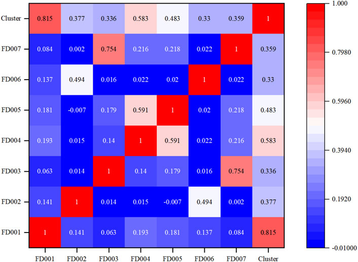
The power correlation coefficient between the cluster and each farm is shown in Figure 7. The cluster is divided into four clusters according to the correlation coefficient thermal map. Wind farm FD001 has a very low correlation with other wind farms, so it is regarded as a cluster alone; wind farms FD002 and FD006 are classified as a cluster; wind farms FD003 and FD007 are classified as a cluster; and wind farms FD004 and FD005 are classified as a cluster. The reference wind farms in each sub-cluster is selected according to the correlation between wind farms and clusters, and the final reference wind farms are FD001, FD002, FD004, and FD007.

FIGURE 7

FIGURE 7. Power correlation coefficient heat map between the cluster and each farm.

4.2 Transitional weather classification and optimal feature selection

In the four types of transitional weather mentioned in Section 2.3, the high wind speed fluctuation weather, according to the wind speed sequence and the actual conditions of each wind farm, has the normalized wind speed of 0.3 selected as the minimum threshold and 0.6 selected as the peak threshold. In this interval, the period of time that meets the conditions of high wind speed fluctuation can be determined as a high wind speed fluctuation process, without using the CBAMSO-XGB model for classification.

Weather conditions except low-temperature icing weather, high-temperature weather, and heavy precipitation weather are uniformly marked as other types of weather. The above four weather types manually marked in the sample are sequentially marked as weather types 1–4 and assigned to the training and test sets in a 7:3 ratio. The number of populations and the maximum number of iterations are 50. The CBAMSO-XGB model is trained with the classification error rate as the objective function. After the classification is completed, high wind speed fluctuation weather is extracted in other types of weather to avoid the interference of high wind speed fluctuation weather on the other three types of weather classification.

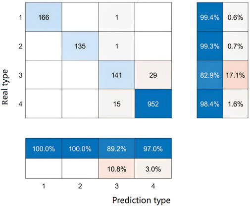
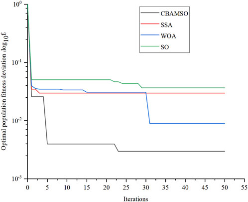
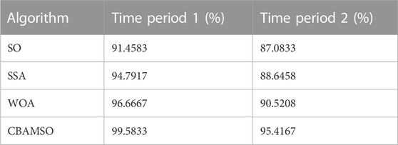
Taking the FD007 reference wind farm as an example, Figures 8A, B show the classification results of the CBAMSO-XGB model for the weather of Periods 1 and 2, respectively, and the overall classification accuracy is relatively high. Time period 1 contains 480 sampling points, time period 2 contains 960 sampling points, and the sampling frequency is 15 min. The overall confusion matrix of the two periods is shown in Figure 9. It can be seen that the model has higher classification accuracy for weather types 1, 2, and 4, and the classification accuracy of weather type 3 is relatively lower. Compared to SO before improvement, SSA, and WOA under the same parameter configuration, the convergence curves of the algorithms are shown in Figure 10. The classification accuracy is shown in Table 4.

FIGURE 8

FIGURE 8. Classification results of the CBAMSO-XGB model for the weather of Periods 1 (A) and 2 (B).

FIGURE 9

FIGURE 9. Overall confusion matrix of the two periods.

FIGURE 10

FIGURE 10. Convergence curves of CBAMSO, SO, SSA, and WOA.

TABLE 4

TABLE 4. Comparison of classification accuracy of different algorithms.

Combined with the analysis of Figure 10 and Table 4, it can be seen that the optimal individual fitness value of the CBAMSO algorithm proposed in this paper is less than 0.003, which is better than the other three algorithms, and the number of iterations is also lower than the other three algorithms. The classification accuracy of CBAMSO in the transitional weather of the two test periods is 99.5833% and 95.4167%, respectively, which is higher than SO, SSA, and WOA. Hence, it is proved that the Bernoulli chaotic map and the bidirectional adaptive Cauchy mutation strategy proposed in this paper effectively improved the convergence speed and classification accuracy of SO.

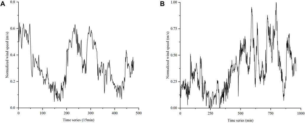
The normalized high wind speed fluctuation curves of Periods 1 and 2 are shown in Figures 11A, B, respectively. Weather type 4 with no precipitation, no icing, and no high temperature is selected to extract the high wind speed fluctuation period. Weather with high wind speed fluctuations can be determined if the high wind speed fluctuation interval includes the lowest threshold of 0.3 and the highest threshold of 0.6. The weather classification results of Periods 1 and 2 after extraction are shown in Figures 12A, B, respectively, where weather type 5 is the high wind speed fluctuation weather.

FIGURE 11

FIGURE 11. Normalized high wind speed fluctuation curves of Periods 1 (A) and 2 (B).

FIGURE 12

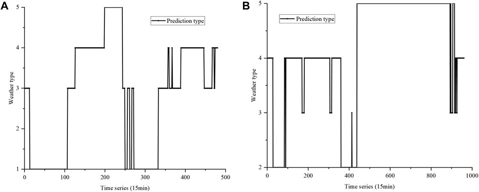
FIGURE 12. Weather classification results of Periods 1 (A) and 2 (B) after extracting the high wind speed fluctuation weather.

4.3 Model prediction and result analysis

The features for transitional weather scenarios are optimized. The correlation coefficient heat maps of the features of high wind speed fluctuation weather, low-temperature icing weather, high-temperature weather, and heavy precipitation weather are shown in Figures 13A–D, respectively.

FIGURE 13

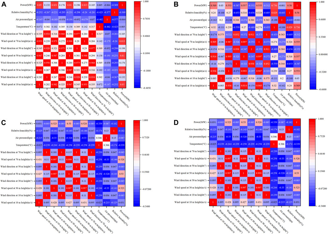
FIGURE 13. Correlation coefficient heat maps of the features of high wind speed fluctuation weather (A), low-temperature icing weather (B), high-temperature weather (C), and heavy precipitation weather (D).

Under the high wind speed fluctuation weather condition, the correlation between wind speed and power is far greater than other features, and the optimized features are wind speed at each height. Under the low-temperature icing weather condition, the correlation between wind speed and power is weakened, and the correlation between temperature and power and that between relative humidity and power are enhanced. Optimized features are wind speed at each selected height, temperature, and relative humidity. Under the high-temperature weather condition, the wind speed is at a lower level, so the optimized features are wind speed at heights 30 m, 50 m, and 70 m and temperature. Under the heavy precipitation weather condition, according to the correlation coefficient heat map, the optimized features are wind speed at each selected height, air pressure, and relative humidity.

A three-layer spatial pyramid pool is constructed according to the optimized features, and the feature dimension of CNN output to LSTM to 9 is fixed. The three-layer spatial pyramid pooling layer divides the feature maps obtained by convolution of the input of any dimension into two, three, and four parts and performs maximum pooling on each part, respectively, and the results obtained by the three-layer spatial pyramid pooling are spliced to obtain the fixed-dimensional features that are finally input into LSTM.

The large sample data are assigned to training and testing samples in an 8:2 split to allow for an adequate inclusion of a wide range of transitory weather. The prediction results of the CNN–LSTM model without feature optimization, the SPP–CNN–LSTM model after feature optimization, and the SPP–CNN–LSTM–ATT model proposed in this paper are compared in Periods 1, 2, and 3, as shown in Figures 14A–C, respectively. Among them, time period 1 includes 192 sampling points within 48 h of reference wind farm FD007, in which sampling points 19–37 and 118–128 are high-temperature weather and 38–117 and 129–167 are high wind speed fluctuation weather; time period 2 is heavy precipitation weather; and time period 3 includes 96 sampling points within 24 h of reference wind farm FD004, in which sampling points 1–60 are low-temperature icing weather.

FIGURE 14

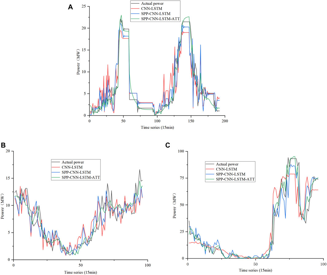
FIGURE 14. Prediction results of the CNN–LSTM model without feature optimization (A), the SPP–CNN–LSTM model after feature optimization (B), and the SPP–CNN–LSTM–ATT model proposed in this paper (C) in three periods.

The mean absolute error (MAE) and root mean square error (RMSE) are used as evaluation indicators. The prediction results of the three models under various transitional weather conditions are shown in Table 5. Analyzing the prediction results and errors of each model, it can be seen that the MAE of the SPP–CNN–LSTM–ATT model proposed in this paper is between 0.9365 and 1.7661, and the RMSE is between 2.0776 and 7.0962, which is much smaller than the corresponding error of the CNN–LSTM and SPP–CNN–LSTM models, and the prediction accuracy is significantly improved. Hence, it is proved that the SPP structure and attention mechanism designed in this paper fully learn the important features of spatial and continuous time dimensions and have good prediction performance for transitional weather.

TABLE 5

TABLE 5. Comparison of the prediction results of three models in the transitional weather period.

The prediction error results of the SPP–CNN–LSTM–ATT model for each reference wind farm, i.e., cluster without upscaling and cluster with upscaling, are shown in Table 6, where the cluster power without upscaling is obtained by the direct summation of the power predictions of seven wind farms within it and the cluster power with upscaling is calculated based on the predictions of the reference wind farms, as shown in Eqs 2, 3. The comparison between the predicted power of the cluster without and with upscaling and the actual power of cluster is shown in Figure 15. Due to the existence of moments of very low wind power in individual wind farms, the errors at these points have a negative impact on the overall accuracy assessment, so the evaluation indexes are MAE and relative root mean square error (RRMSE). The cluster power value obtained by upscaling the power predictions of the reference wind farm contains less redundant information and can be seen to have a lower error than the cluster power value obtained by direct accumulation. The combined analysis of MAE and its corresponding installed capacity, as well as the analysis of RRMSE, due to the smoothing effect of the cluster, and the cancellation effect of the volatility of each wind farm contribute to the higher prediction accuracy of the cluster than the individual wind farms.

TABLE 6

TABLE 6. Comparison of the prediction results of reference wind farms and cluster.

FIGURE 15

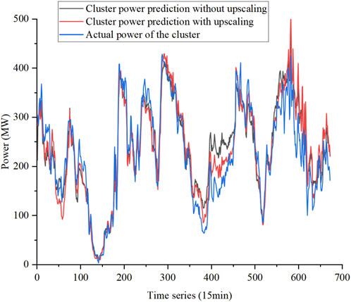
FIGURE 15. Comparison of the predicted power of the cluster without and with upscaling and the actual power of the cluster.

5 Conclusion

The specific contributions of the CBAMSO-XGB–SPP–CNN–LSTM–ATT model proposed in this study are as follows:

(1) The CBAMSO algorithm proposed in this paper achieves a fast and accurate classification of transitional weather, and the classification accuracy of CBAMSO in the transitional weather of the two periods is 99.5833% and 95.4167%, respectively, which is higher than SO, SSA, and WOA. Compared with CNN–LSTM and SPP–CNN–LSTM models, the MAE and RMSE of the proposed model in each transitional weather period are approximately reduced by 42.49%–72.91% and 65.34%–91.22%, respectively. The above strategies have been shown to solve the problem of lack of detailed analysis of influencing factors in wind power prediction of transitional weather and the problem of ignoring time continuity by modeling separately, which effectively improves the prediction accuracy.

(2) There is error complementarity between wind farms in the cluster. The reference wind farm for upscaling accurately and effectively maps cluster power, and the cluster wind power prediction error is lower than the prediction error of each reference wind farm. The above strategies have been shown to solve the problem of focusing on the power prediction of a single wind farm and the lack of analysis of the whole wind farm cluster, and the power accuracy of the cluster is higher.

However, there are still some limitations to this study. The accuracy of wind power prediction depends on data quality. Meteorological data on transitional weather are abnormal compared with those on normal weather. It is easy to be eliminated by the quartile method as the wrong data, and the recovery and correction of the eliminated data are also limited. Using more accurate NWP acquisition data and abnormal data cleaning correction method can effectively improve the prediction accuracy. Due to the limitation of data, this paper divides transitional weather into four categories, which are relatively limited. The next work will further study the influence mechanism of transitional weather on the operation of wind turbines and whether it is applicable to other regions so as to make a more detailed division of weather types. In addition to the necessary meteorological and historical power data, the next research will consider the introduction of wind turbine internal features, virtual power plants, and other features to further improve the prediction accuracy.

Data availability statement

The raw data supporting the conclusion of this article will be made available by the authors, without undue reservation.

Author contributions

GD: conceptualization, data curation, methodology, resources, and writing–review and editing. GY: conceptualization, data curation, methodology, resources, and writing–review and editing. ZW: formal analysis, validation, writing–review and editing. BK: formal analysis, validation, and writing–review and editing. ZX: visualization and writing–review and editing. XZ: visualization and writing–review and editing. HX: writing–original draft and writing–review and editing. WH: writing–original draft and writing–review and editing.

Funding

This work was supported by the Jiangxi Provincial Department of Education Science and Technology Project (GJJ211943).

Acknowledgments

The authors acknowledge these supports gratefully.

Conflict of interest

The authors declare that the research was conducted in the absence of any commercial or financial relationships that could be construed as a potential conflict of interest.

Publisher’s note

All claims expressed in this article are solely those of the authors and do not necessarily represent those of their affiliated organizations, or those of the publisher, the editors, and the reviewers. Any product that may be evaluated in this article, or claim that may be made by its manufacturer, is not guaranteed or endorsed by the publisher.

Supplementary material

The Supplementary Material for this article can be found online at: https://www.frontiersin.org/articles/10.3389/fenrg.2023.1253712/full#supplementary-material

References

Fu, Y. W., Hu, W., Tang, M. L., Yu, R., and Liu, B. S. (2018). Multi-step ahead wind power forecasting based on recurrent neural networks in 2018 IEEE PES Asia-Pacific Power and Energy Engineering Conference (APPEEC) (IEEE), 217–222. doi:10.1109/APPEEC.2018.8566471

CrossRef Full Text

Gong, Z. W. Y., Ma, X. L., Xiao, N., Cao, Z. G., Zhou, S., Wang, Y. L., et al. (2022). Short-term power prediction of a wind farm based on empirical mode decomposition and mayfly algorithm–back propagation neural network. Front. Energy Res. 10. doi:10.3389/FENRG.2022.928063

CrossRef Full Text | Google Scholar

Hashim, F. A., and Hussien, A. G. (2022). Snake Optimizer: a novel meta-heuristic optimization algorithm. Knowledge-Based Syst. 242, 108320. doi:10.1016/J.KNOSYS.2022.108320

CrossRef Full Text | Google Scholar

Huang, F., Jia, R. Y., Bai, S. X., and You, H. (2022). New design of short-term wind power forecasting algorithm based on VMD-grid-SVM. Front. Power Energy Syst. 1 (1), 1–9. doi:10.23977/FPES.2022.010101

CrossRef Full Text | Google Scholar

Kim, Y. J., and Byun, Y. C. (2022). Ultra-short-term continuous time series prediction of blockchain-based cryptocurrency using LSTM in the big data era. Appl. Sci. 12 (21), 11080. doi:10.3390/APP122111080

CrossRef Full Text | Google Scholar

Li, Z. S., and Liu, Z. G. (2019). Feature selection algorithm based on XGBoost. J. Commun. 40 (10), 101–108. doi:10.11959/j.issn.1000-436x.2019154

CrossRef Full Text | Google Scholar

Liu, F., Wang, Z., Liu, R. D., and Wang, K. (2021). Short-term forecasting method of wind power generation based on BP neural network with combined loss function. J. Zhejiang Univ. Sci. 55 (3), 594–600. doi:10.3785/j.issn.1008-973X.2021.03.021

CrossRef Full Text | Google Scholar

Liu, H., Yang, L. X., Zhang, B. Y., and Zhang, Z. J. (2023). A two-channel deep network based model for improving ultra-short-term prediction of wind power via utilizing multi-source data. Energy 283, 128510. doi:10.1016/j.energy.2023.128510

CrossRef Full Text | Google Scholar

Liu, H., and Zhang, Z. J. (2022). A bilateral branch learning paradigm for short term wind power prediction with data of multiple sampling resolutions. J. Clean. Prod. 380, 134977. doi:10.1016/j.jclepro.2022.134977

CrossRef Full Text | Google Scholar

Mohamad, A. H., Hamza, Z. M., Majad, M., and Chen, W. J. (2023). COA-CNN-LSTM: coati optimization algorithm-based hybrid deep learning model for PV/wind power forecasting in smart grid applications. Appl. Energy 349, 121638. doi:10.1016/j.apenergy.2023.121638

CrossRef Full Text | Google Scholar

Peng, X. S., Xiong, L., Wen, J. Y., Cheng, S. J., Deng, D. Y., Feng, S. L., et al. (2016). A summary of the state of the art for short-term and ultra-short-term wind power prediction of regions. Proc. CSEE 36 (23), 6315–6326+6596. doi:10.13334/j.0258-8013.pcsee.161167

CrossRef Full Text | Google Scholar

Shahram, H., Saeid, L., Hossein, Z., and Andrea, C. (2022). Offshore wind power forecasting—a new hyperparameter optimisation algorithm for deep learning models. Energies 15 (19), 1–21. doi:10.3390/EN15196919

CrossRef Full Text | Google Scholar

Su, W., Jiang, F., Shi, C. Y., Wu, D. Q., Liu, L., Li, S. H., et al. (2023). An XGBoost-based knowledge tracing model. Int. J. Comput. Intell. Syst. 16 (1), 13. doi:10.1007/S44196-023-00192-Y

CrossRef Full Text | Google Scholar

Wang, J. N., Zhu, H. Q., Zhang, Y. J., Cheng, F., and Zhou, C. (2023). A novel prediction model for wind power based on improved long short-term memory neural network. Energy 265, 1373–1388. doi:10.1016/J.ENERGY.2022.126283

CrossRef Full Text | Google Scholar

Wang, Y. J., Lu, Z. X., Qiao, Y., Wu, L. L., and Xu, H. X. (2017). Short-term regional wind power statistical upscaling forecasting based on feature clustering. Power Syst. Technol. 41 (5), 1383–1389. doi:10.13335/j.1000-3673.pst.2017.0326

CrossRef Full Text | Google Scholar

Wang, Y. R., Wang, D. C., and Tang, Y. (2020). Clustered hybrid wind power prediction model based on ARMA, PSO-SVM, and clustering methods. IEEE Access 8, 17071–17079. doi:10.1109/access.2020.2968390

CrossRef Full Text | Google Scholar

Xiong, Z. H., Chen, Y., Ban, G. H., Zhuo, Y. X., and Huang, K. (2022). A hybrid algorithm for short-term wind power prediction. Energies 15 (19), 7314–7411. doi:10.3390/EN15197314

CrossRef Full Text | Google Scholar

Xue, Y. S., Chen, N., Wang, S. M., Wen, F. S., Lin, Z. Z., and Wang, Z. (2017). Review on wind speed prediction based on spatial correlation. Automation Electr. Power Syst. 41 (10), 161–169. doi:10.7500/AEPS20170109002

CrossRef Full Text | Google Scholar

Yang, Z. M., Peng, X. S., Lang, J. X., Wang, H. Y., Wang, B., and Liu, C. (2021). Short-term wind power prediction based on dynamic cluster division and BLSTM deep learning method. High. Volt. Eng. 47 (4), 1195–1203. doi:10.13336/j.1003-6520.hve.20210079

CrossRef Full Text | Google Scholar

Ye, L., Zhang, C. H., Tang, Y., Sun, B. H., Zhong, W. Z., Lan, H. B., et al. (2018). Active power stratification predictive control approach for wind power cluster with multiple temporal and spatial scales coordination. Proc. CSEE 38 (13), 3767–3780+4018. doi:10.13334/j.0258-8013.pcsee.171685

CrossRef Full Text | Google Scholar

Ye, L., and Zhao, Y. N. (2014). A review on wind power prediction based on spatial correlation approach. Automation Electr. Power Syst. 38 (14), 126–135. doi:10.7500/AEPS20130911004

CrossRef Full Text | Google Scholar

Yu, G. Z., Lu, L., Tang, B., Wang, S. Y., and Dong, Q. (2022). Research on ultra-short-term subsection forecasting method of offshore wind power considering transitional weather. Proc. CSEE 42 (13), 4859–4871. doi:10.13334/j.0258-8013.pcsee.211771

CrossRef Full Text | Google Scholar

Yue, X. Y., Peng, X. G., and Lin, L. (2020). Short-term wind power forecasting based on whales optimization algorithm and support vector machine. Proc. CSU-EPSA 32 (2), 146–150. doi:10.19635/j.cnki.csu-epsa.000249

CrossRef Full Text | Google Scholar

Zeng, Q., and Chen, Z. H. (2019). A review of the effect of meteorological disasters on wind farms in recent years. Adv. Meteorological Sci. Technol. 9 (2), 49–55. doi:10.3969/j.issn.2095-1973.2019.02.010

CrossRef Full Text | Google Scholar

Zhang, J. A., Liu, D., Li, Z. J., Han, X., Liu, H., Dong, C., et al. (2021). Power prediction of a wind farm cluster based on spatiotemporal correlations. Appl. Energy 302, 117568. doi:10.1016/J.APENERGY.2021.117568

CrossRef Full Text | Google Scholar

Zhang, Y., Wang, P., Ni, T., Cheng, P., and Lei, S. (2017). Wind power prediction based on LS-SVM model with error correction. Adv. Electr. Comput. Eng. 17 (1), 3–8. doi:10.4316/AECE.2017.01001

CrossRef Full Text | Google Scholar

Zhao, H. S., Yan, X. H., Wang, G. L., and Yin, X. L. (2019). Fault diagnosis of wind turbine generator based on deep autoencoder network and XGBoost. Automation Electr. Power Syst. 43 (1), 81–86. doi:10.7500/AEPS20180708001

CrossRef Full Text | Google Scholar

Zhao, Y. N., Ye, L., and Zhu, Q. W. (2014). Characteristics and processing method of abnormal data clusters caused by wind curtailments in wind farms. Automation Electr. Power Syst. 38 (21), 39–46. doi:10.7500/AEPS20131213010

CrossRef Full Text | Google Scholar