 Sha Liu
 Cheng Chang1
 Hong Li
- 1Shale Gas Research Institute, PetroChina Southwest Oil and Gas Field Branch, Chengdu, Sichuan, China
- 2CCDC Sulige Project Management Department, Erdos, China
To effectively develop the shale gas in the southern Sichuan Basin, it is essential to accurately predict and evaluate the single-well production and estimated ultimate recovery (EUR). Empirical production decline analysis is most widely used in predicting EUR, since it is simple and can quickly predict the gas well production. However, this method has some disadvantages, such as many parameters of the model, difficulty in fitting and large deviation. This paper presents an efficient process of EUR prediction for gas wells based on production decline models. Application of nine empirical production decline models in more than 200 shale gas wells in the Changning block of the Sichuan Basin was systemically analyzed. According to the diagnosis of flow regime, it was determined that all models are applicable in the prediction of production and EUR in this area, with the fitting degree higher than 80% for gas wells producing for more than 12 months. Based on the fitting and prediction results, the parameter distribution charts of the nine production decline models with initial parameters constrained were plotted for shale gas wells, which greatly improved the prediction accuracy and efficiency. Coupled with the probability method, the EUR was evaluated and predicted effectively, and the average EUR of more than 200 shale gas wells in the Changning block is 1.21 × 10⁸ m3. The EUR of Well CNH1 predicted by the proposed process and charts is believed reliable. The study results provide meaningful guidance for the efficient prediction of gas well production and EUR in the Changning block.
1 Introduction
As a hot spot in unconventional gas exploration and development, shale gas has renovated the energy framework in the United States and around the world. In China, with the transformation of the economy from rapid development to high-quality development and the adjustment of energy structures, the demand for clean energy represented by natural gas is increasing. According to a global survey by the U.S. Energy Information Administration (EIA), the shale gas reserves in China are about 31.6 × 10¹² m3 (ElA’s, 2019), suggesting a major option for gas production in the country. With focus on the marine shale areas shallower than 3,500 m in the Sichuan Basin, China produced 240 × 108 m3 of shale gas in 2022 (Liu et al., 2023).
Through trials and tests in recent years, significant breakthroughs have been made in the exploration of marine shales in the Ordovician Wufeng formation–Silurian Longmaxi formation (“Wufeng–Longmaxi”) in the Sichuan Basin. Typically, in Changning, a major block of the Changning–Weiyuan National Shale Gas Demonstration Area, the technology for effective development of marine shale gas layers shallower than 3,500 m has been formed, which allows the EUR per well to increase gradually, providing a valuable basis for production allocation, working system optimization, and new well drilling (Ma and Xie, 2018; Xie, 2018). Nevertheless, as a kind of self-generating and self-storing artificial gas reservoir, shale gas reservoirs are developed by “long horizontal well + volume fracturing,” and the gas seepage mechanism is complex. These bring difficulties in the analysis of shale gas production decline and EUR prediction. Scholars have analyzed and predicted the production performance of shale gas wells by using various methods, such as the experimental results analysis (Xu et al.; Xu et al., 2023), analytical and numerical simulation (Samandarli et al., 2011; Stalgorova and Mattar, 2012), data-driven production decline curve analysis (Fetkovich, 1973; Blasingame et al., 1991), and machine learning and artificial intelligence algorithms (Wang et al., 2018; Zeng et al., 2018; Wang et al., 2021; LuoDingCheng et al., 2022; Wang et al., 2023). The analytical methods take into account complex seepage mechanisms and rock–fluid interactions such as adsorption, desorption, slippage, and diffusion effects (Yao et al., 2013; Du et al., 2021; Cui et al., 2023). However, the analytical and numerical simulation methods are computationally expensive, difficult, and time-consuming; also, a complete set of parameters required by analytical models are hard to obtain, and their prediction results are highly dependent on the accuracy of input parameters. In contrast, the data-driven production decline model is simple and efficient in predicting shale gas production and provides quick and reasonable prediction of production, so it is most widely used in EUR prediction. However, it involves a large number of parameters and the unclear value range of initial fitting parameters, possibly causing a large deviation between the prediction result and the actual production. Thus, the range of the model parameters should be clarified to ensure the prediction accuracy.
Taking shale gas wells in the Changning block as examples, and based on the field production data, the deviation in production fitting and prediction using empirical production decline models were analyzed, and the range of model parameters was defined. The probability method is considered reasonable in the EUR evaluation of shale gas wells. The study results provide a reference for reservoir engineers to adjust the production decline model, and also guide the high-quality, large-scale, and effective development of shale gas and production evaluation in the southern Sichuan Basin.
2 Geological setting
The Changning block in the low gentle structural belt, southern Sichuan Basin, includes the Changning anticline, without faults in the main part. Vertically, there are six sets of marine and continental shale strata, among which the favorable strata are the Lower Cambrian Qiongzhusi Fm and the Ordovician Wufeng Fm–Silurian Longmaxi Fm (“Wufeng–Longmaxi”). The major target interval from the Wufeng Fm to the first sub-member of the first member of the Longmaxi Fm (“L11”) is composed of black siliceous carbonaceous shale and organic-rich black carbonaceous shale of outer shelf subfacies. In Wufeng–Longmaxi, most of strata are buried at depths of less than 3,500 m, and the high-quality shale is distributed continuously and stably with a thickness of about 30–60 m. The source rocks are highly enriched. The reservoir rocks are characterized by high Total Organic Carbon, high gas content, high brittleness, and medium porosity. The pressure system is basically overpressure, suggesting a good gas storage condition. The physical properties and gas-bearing properties vary slightly within the same interval. Therefore, Wufeng–Longmaxi is the major series of development strata and also the principal source of commercial shale gas productivity (Yang et al., 2016; Ma and Xie, 2018).
The establishment of the Changning–Weiyuan National Shale Gas Demonstration Area in 2012 inaugurated a new journey in the efficient development of shale gas in the southern Sichuan Basin. By 2022, in the Changning block, over 510 wells had been put into production, revealing a single-well decline rate of about 50% in the first year of production. The Changning block has become a major shale gas province, with the daily production over 1,500 × 104 m3 and the annual production over 50 × 108 m3.
3 Production decline analysis method
3.1 Empirical production decline models
The characteristics of the production stage of shale gas wells are easy to observe; the production has an obvious decline phenomenon, mainly showing rapid initial decline and then, with the passage of time, generally 6-12 months, there is a slow decrease, and the overall has obvious “long tail” behavior.
Over the years, production decline models for shale gas wells have emerged one after another and been used widely. Arps (1945) proposed the approach for analyzing production decline with empirical formulas, and developed exponential decline, hyperbolic decline, and harmonic decline models according to the production data of actual gas wells, which enable the qualification of production decline of gas wells. Later, other scholars put forward more production decline curve analysis methods. Ilk et al. (2008) proposed a power-law exponential decline (PLE) method for shale gas wells in North America, and verified the method with numerical simulation data and actual data. Valko (2009) proposed the stretched exponential production decline (SEPD) method for shale gas wells, and applied it with the production data of Barnett shale gas wells in North America. Duong (2010) indicated that long term fracture linear flow exists in gas well production process, and proposed a production decline analysis model for wells in fractured shale gas reservoirs, or the DUONG model, which has also been satisfactorily used in Barnett gas wells. Clark (2011) adopted the logistic growth model (LGM) to predict shale gas production. Duong found that the log–log curve of the ratio of daily gas production to cumulative gas production versus time is a straight line when the flow in fractures is dominant (Duong, 2011), and he proposed a modified DUONG method applicable in EUR prediction in linear flow and boundary-dominated flow by adjusting the empirical analysis (Duong, 2014). Zhang et al. (2016) proposed an extended exponential decline curve analysis (EEDCA) method for shale gas reservoirs based on field data. Qi et al. (2016) established a hyperbolic-exponential hybrid decline (HEMD) model based on Ilk’s PLE model. Wang et al. (2017) proposed a new production decline model (the Wang model) based on the basic theories of the Arps, SEPD, and DUONG methods to predict the production and EUR of gas wells in fractured reservoirs. Gupta et al. (2018) revised the Arps exponential decline equation and proposed a variable exponential decline-modified (VDMA) model for analyzing the production decline in shale gas reservoirs. From 2020 to 2022, based on the above models, many scholars derived or re-established the production decline model of shale gas wells considering different factors. However, in practical application, the production data need to be complicated and have not been widely used on a large scale (BAO, 2022; Hao et al., 2022). These models have their respective application conditions and scope, and thus should be used properly depending on the actual production performance of shale gas wells. Most models ensure accurate prediction when the boundary flow state is reached in gas wells. Table 1 compares these models.

TABLE 1. Comparison of empirical production decline models.
3.2 Workflow of data analysis and processing
3.2.1 Preprocessing of production data
The empirical production decline model is mainly applied in the production decline stage. To apply the model effectively and accurately, it is necessary to preprocess the production data as follows:
1) Eliminate the data in the early non-decline stage to improve the fitting accuracy of the empirical model (the portion of gas production that was eliminated prior to analysis will be added to projected total cumulative gas production), so that the production and EUR of gas wells can be predicted more accurately;
2) Eliminate the data at the zero-production points in the period of shut-in which is possibly done for production arrangement, workover, or other purposes, so that the data continuity can be maintained to realize a higher fitting accuracy.
The specific data processing process is shown in Figure 1.
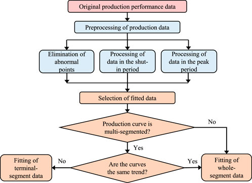
FIGURE 1. Workflow of data analysis and processing.
3.2.2 Selection of fitted data segment
Four production decline typical curves are shown in Figure 2 (the abscissa in the figure indicates the production time of shale gas wells, and the ordinate indicates the gas well production; ① represents the trend of the first curve and ② represents the trend of the second curve). When the shale gas well maintains continuous and stable production, the curve characteristics are mainly shown in Figure 2A. If the gas well is temporarily shut in due to uncontrollable factors such as on-site workover, the curve characteristics may be as shown in Figure 2B. If the choke size of the gas well is temporarily adjusted (reduced) due to production management requirements in the production process, the curve characteristics may be as shown in Figure 2C. If the production decline trend changes due to the influence of technological measures and inter-well interference during the production of gas wells, the curve characteristics may be as shown in Figure 2D. For the curves in Figures 2A–C, i.e., the overall production data fall on one trend line (as one-segment distribution), the effect of a temporary increase or decrease of production on the predicted EUR can be ignored, and the whole-segment data are selected for fitting with the empirical model. For the curve in Figure 2D, which is multi-segmented, the production data of the terminal segment are selected for fitting.
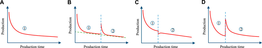
FIGURE 2. Production decline type curves (① represents the trend of the first curve and ② represents the trend of the second curve); (A–D) represent four possible production curve characteristics of shale gas Wells, respectively; the green dashed line represents the change trend of the production curve, and the blue dashed line represents the point of sudden change of the production curve.
3.3 Analysis of deviation in model fitting and prediction
Generally, the parameters of production decline models are obtained through equation linearization or numerical computation (e.g., non-linear least squares method) (Zhang et al., 2012). There are three or more unknown parameters in the models in Table 1, except in the Wang model. This makes equation linearization very difficult. The non-linear least square method has no special requirements on the model parameters. Thus, it is popular that non-linear regression is incorporated into the fitting of production data in multi-parameter models. In least squares fitting analysis, the determination coefficient or goodness of fit R2 is used to measure the difference between the actual data and the fitted value. The value of R2 is taken as the fitting accuracy and expressed as:
where
The analysis of fitting effect and deviation for gas wells with a production history of more than 12 months with the empirical production decline models in Table 1 provides a basis for the optimization of the empirical model and accurate prediction of the EUR. The fitting effects of more than 200 shale gas wells with a production history of more than 12 months in the Changning block were analyzed. As shown in Figure 3, the R2 of all nine models is above 0.8, and the fitting deviation is small and is within the acceptable range. This indicates that the empirical models have good adaptability to the production of shale gas wells and guarantee the accuracy of subsequent EUR prediction.
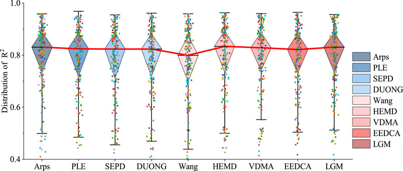
FIGURE 3. Distribution of fitting deviation.
The duration of production data is different for gas wells that are put into production at different times. To track and predict the production and EUR of gas wells at different production times for providing a reference to the improvement of the development effect, it is necessary to understand the fitting and prediction accuracy of the empirical model at different production times. The differences in fitting and prediction of production by the same model at different times were analyzed to determine the best fitted production time, improve the applicability of the empirical model, and enhance the accuracy in predicting EUR. We used a similar prior approach to split the actual gas production data into two parts of historical production data. The first part of historical production data was used to fit and obtain model parameters, which were used to predict gas production, and the second part of historical production data was used to compare with the predicted gas production, so as to verify the accuracy of the model prediction. If the predicted value is closer to the actual value, the prediction deviation is smaller, and the model is more accurate. The prediction deviation is characterized by the standard deviation, or root mean square error (RMSE). RMSE is always used as a standard for measuring the prediction results of machine learning models and the deviation between the predicted value and the actual value. RMSE is expressed as:
where
3.4 Analysis of uncertainty in EUR prediction using the probability method
All nine production decline models mentioned are applicable to shale gas wells. In practice, the predicted production is constrained to a reasonable range by controlling the value of the model parameters. Nevertheless, there are large differences in the prediction results from multiple models. Measurement of the uncertainty in the prediction results is of great significance to ensure the highest accuracy of predicted production of gas wells and provide a basis for the evaluation of gas production and decision-making in investment. According to the definition of reserves by the Society of Petroleum Engineers (SPE) and the United States Securities and Exchange Commission (SEC) in 1997, the probability method can be used as a tool for evaluating oil and gas resources (Jia et al., 2009) and it has been widely used around the world. The probability method is one of the conventional methods for the estimation of resource/reserves and evaluation of predicted EUR reliability. In this paper, the probability method was integrated with the cumulative distribution function (CDF) to describe the probability distribution of the prediction results from different production decline models and evaluate the uncertainty in prediction results (Figure 4).
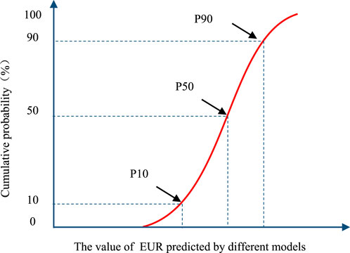
FIGURE 4. Distribution of cumulative probability. (The abscissa indicates the different EUR values of gas wells predicted by different production decline models, and the ordinate indicates the cumulative probability percentage of these EUR values.)
In the evaluation of the EUR of shale gas wells with the probability method here, the cumulative probability P10, P50, and P90 values in the evaluation criteria are used as the EUR evaluation level. The P90 value indicates the optimistic result, the P50 value indicates the best result, and the P10 value indicates the conservative result. The P50 value will serve as the final gas well EUR, further reducing the uncertainty of the gas well EUR forecast, helping shale gas companies to reasonably calculate the return on investment of shale gas, and supporting effective development technology decisions. At the same time, the values of P10-P90 are used as the EUR range of gas wells to understand the possible risks of shale gas production.
4 Discussion
4.1 Production fitting and prediction result
4.1.1 Diagnosis of flow regime in typical wells
To analyze the application effect of the Arps, PLE, SEPD, DUONG, EEDCA, Wang, HEMD, VDMA, and LGM models, the production data from more than 200 shale gas wells in the Changning block were analyzed, and the P10, P50, and P90 typical curves were obtained after calculation. P10 is a cumulative probability of 10% and means that the daily gas production in this typical curve has at least 10% reliability, and P50 and P90 have a similar meaning to P10 (Figure 5). To meet the conditions for the application of models, diagnosis of the flow regime was performed in the typical curve, and the linear flow regime with the slope of −1/2 and the boundary flow regime with the slope of −1 were determined (Figure 6). It was judged that the time for the gas wells to reach boundary-dominated flow regimes was not less than 12 months. More than 200 gas wells that have reached the boundary-dominated flow stage were selected from the more than 300 gas wells in the Changning block and analyzed with the nine empirical models illustrated above.
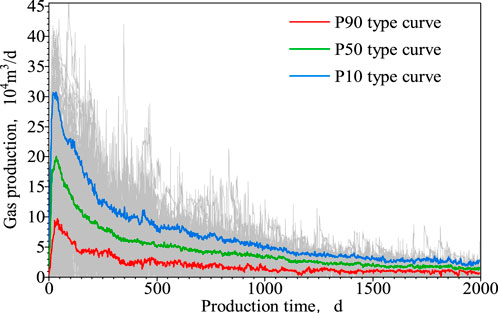
FIGURE 5. Typical curves for the Changning block.
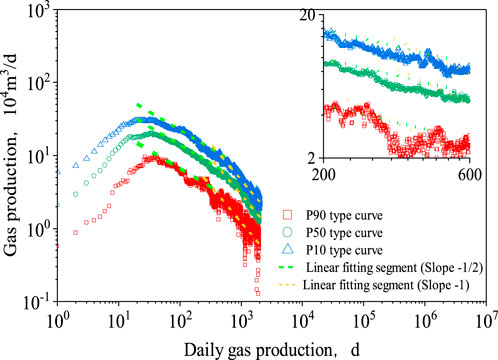
FIGURE 6. Log–log curves for the Changning block.
4.1.2 Analysis of fitting and prediction deviation for typical wells
The P50 typical curves of gas wells in the Changning block were analyzed with the method described in Section 3.2. It can be seen from Figure 7 that the prediction results from the models are different at varied fitted production times. Given the same model, the longer the fitted production time, the better the fitting effect and the smaller the prediction deviation. When the fitted production time reaches 12 months and above, all models have high fitting accuracy and low prediction deviation. It is recommended that the time of production data reaches 12 months when using the model to predict gas production, so as to ensure the accuracy of production and EUR prediction to a certain extent.
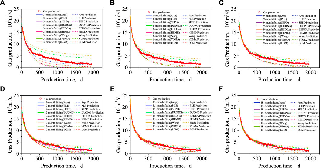
FIGURE 7. Fitted different production times and prediction results; (A–F) represent the production history of 3, 6, 9, 12, 15, and 18 months of fifitting, respectively.
4.1.3 Parameter distribution range
According to the results of production fitting and prediction of shale gas wells, the production decline models have good applicability in production prediction through the fitting algorithm. It should be noted that the non-linear regression algorithm requires a higher accuracy on the initial parameters of the models, and input of initial parameters may cause local optimal in non-linear regression, resulting in large deviation in the historical fitting of gas well production and inaccurate prediction results. Therefore, it is of significance to provide the distribution range of model parameters to constrain the regression algorithm.
The parameter distribution charts of models were obtained by analyzing the data of more than 200 gas wells in the Changning block with the production decline models; some of the models’ parameter distributions are shown in Figures 8–12. The initial parameter range of models was obtained through statistics of the parameters’ distributions (Table 2). Constraint of the referred ranges of the initial parameters of the models provides a reference for application of the production decline models.
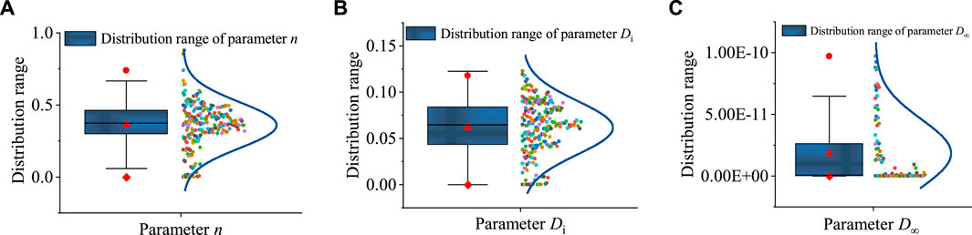
FIGURE 8. Distribution range of parameters of the PLE model; (A–C) represent the distribution ranges of different key parameters in the PLE model.
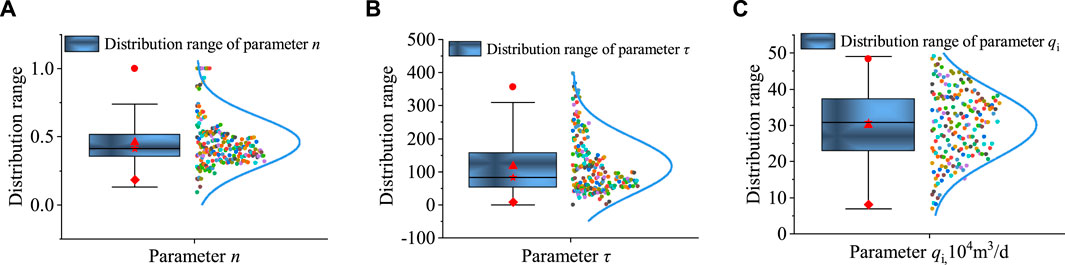
FIGURE 9. Distribution range of parameters of the SEPD model; (A–C) represent the distribution ranges of different key parameters in the SEPD model.
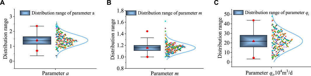
FIGURE 10. Distribution range of parameters of the DUONG model; (A–C) represent the distribution ranges of different key parameters in the DUONG model.
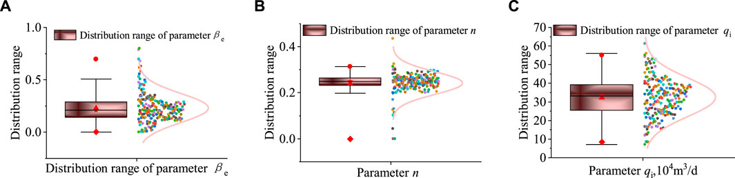
FIGURE 11. Distribution range of parameters of the EEDCA model; (A–C) represent the distribution ranges of different key parameters in the EEDCA model.
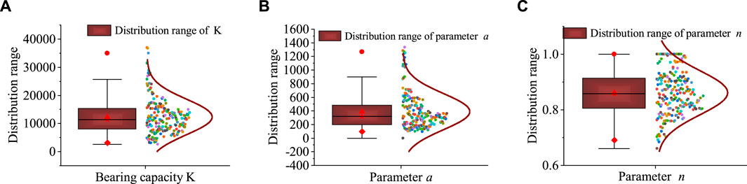
FIGURE 12. Distribution range of parameters of the LGM model; (A–C) represent the distribution ranges of different key parameters in the LGM model.
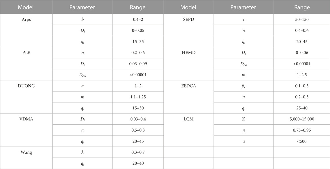
TABLE 2. Distribution of the parameters of models.
4.2 Process of EUR prediction based on production decline models
Based on the analysis results above, a simple and reliable process of shale gas production and EUR prediction for shale gas wells was proposed (Figure 13). It can realize rapid production prediction and accurate EUR evaluation, thus improving the efficiency of production and EUR prediction. Through the EUR prediction process, the efficiency and accuracy of EUR results of more than 200 shale gas wells in the Changning block are realized, and the average EUR of gas wells in this block is predicted to be 1.21 × 10⁸ m3.
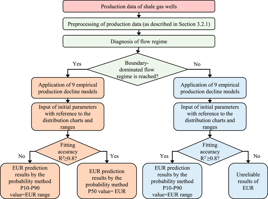
FIGURE 13. Process of EUR prediction based on production decline models.
4.3 Application example
With the above-mentioned production decline models, production prediction was carried out with the production data of Well CNH1 in the Changning block, and the predicted production was compared with the predicted EUR. Based on the historical production data of Well CNH1, the production data after peak production was obtained with the above workflow of data processing. The historical production was fitted by referring to the range of the initial parameters of the models, and the fitting accuracy was higher than 80%. The production and EUR were predicted based on the model parameters (Figures 14, 15). The comparison shows the differences in the EUR prediction results of various models. The probability method was used to analyze the distribution of the EUR predicted by different models, and the P50 value was used as the final EUR, which was 1.25 × 10⁸ m3 (Table 3). Well CNH1 has produced for more than 3 years, with a cumulative gas production of 7,660 × 104 m3. According to the production performance and the recovery percentage, the predicted production is reliable.
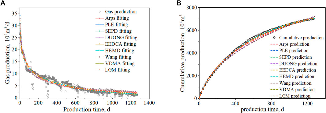
FIGURE 14. Fitted and predicted production of Well CNH1, where (A) represents the fifitting results of the historical gas production of CNH1 by different models and (B) represents the results of gas production prediction of CNH1 by different models.
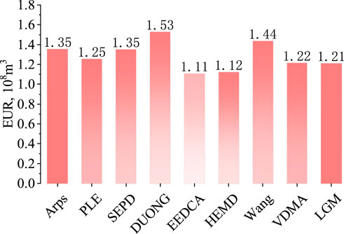
FIGURE 15. Predicted EUR of well CNH1.
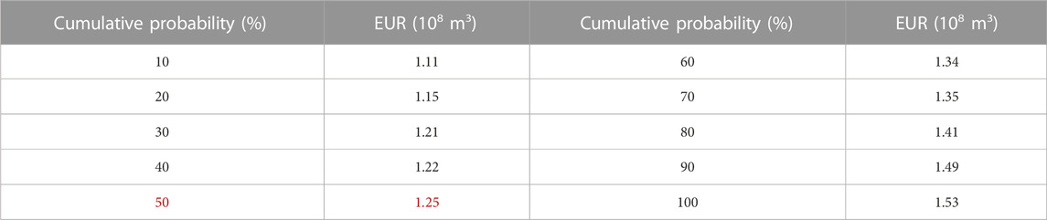
TABLE 3. EUR of Well CNH1 at different cumulative probabilities.
5 Conclusion
After systematic analysis and application of the production decline models for shale gas wells in the Changning block, the process of EUR prediction based on production decline models was proposed. The conclusions are obtained as follows:
1) Diagnosis of flow regime shows that shale gas wells in the Changning block have been producing for more than 12 months, and the Arps, PLE, SEPD, DUONG, Wang, VDMA, HEMD, EEDCA, and LGM models can all be used in the prediction of production and EUR for these wells, with the fitting accuracy higher than 80%.
2) Based on the results of fitting and prediction for more than 200 gas wells, the parameter distribution charts of nine production decline models suitable for shale gas wells in the Changning block were plotted. The initial parameters of the models were constrained to avoid the local optimum in production fitting. Thus, the production and EUR of shale gas wells could be predicted more rationally and efficiently.
3) The process of EUR prediction proposed in this paper was used to fit and predict the production of Well CNH1. The EUR predicted at different cumulative probabilities was obtained. The EUR corresponding to P50 was selected as the final EUR to ensure the highest accuracy of the predicted EUR and provides a basis for the evaluation of gas well production and decision-making in investment.
Data availability statement
The data that support the findings of this study are available from the Shale Gas Research Institute of the PetroChina Southwest Oil and Gas Field Branch. Restrictions apply to the availability of these data, which were used under license for this study. Data are available from the authors with the permission of the Shale Gas Research Institute of the PetroChina Southwest Oil and Gas Field Branch.
Author contributions
SL contributed as the lead author of the article, including conceptualization, methodology, and data processing. CC, WX, and HL determined the context of the article and modified the details of the article. All authors contributed to the article and approved the submitted version.
Funding
The authors acknowledge the financial support of the Shale Gas Research Institute of the PetroChina Southwest Oil and Gas Field Branch (NO. 20220304-16).
Conflict of interest
Authors SL, CC, and WX were employed by Shale Gas Research Institute, PetroChina Southwest Oil and Gas Field Branch.
The remaining author declares that the research was conducted in the absence of any commercial or financial relationships that could be construed as a potential conflict of interest.
The authors declare that this study received funding from the Shale Gas Research Institute of the PetroChina Southwest Oil and Gas Field Branch The funder had the following involvement in the study: data collection, and the decision to submit it for publication.
Publisher’s note
All claims expressed in this article are solely those of the authors and do not necessarily represent those of their affiliated organizations, or those of the publisher, the editors and the reviewers. Any product that may be evaluated in this article, or claim that may be made by its manufacturer, is not guaranteed or endorsed by the publisher.
References
Bao, K. (2022). Variable pressure-variable production decline model and its application in shale gas wells. Unconv. Oil Gas 9 (6), 81–86. doi:10.19901/j.fcgyq.2022.06.12
Blasingame, T. A., McCray, T. L., and Lee, W. J. (1991). “Decline curve analysis for variable pressure drop/variable flowrate systems,” in Proceedings of the paper SPE 21513 presented at the SPE gas technology symposium, Houston, Texas, United States, January 1991, 23–24.
Clark, A. J. (2011). Decline curve analysis in unconventional resource plays using logistic growth models. Master Dissertation. Austin, TX, USA: University of Texas at Austin.
Cui, Q., Zhao, Y., Zhang, L., Chen, M., Gao, S., and Chen, Z. (2023). A semianalytical model of fractured horizontal well with hydraulic fracture network in shale gas reservoir for pressure transient analysis. Adv. Geo-Energy Res. 8 (3), 193–205. doi:10.46690/ager.2023.06.06
Du, D., Zhang, Y., Zhang, L., et al. (2021). Research progress and prospect of seepage mechanism in shale gas reservoirs. Unconv. Oil Gas 8 (3), 1–9. doi:10.19901/j.fcgyq.2021.03.01
Duong, A. N. (2010). “An unconventional rate decline approach for tight and fracture-dominated gas wells,” in Proceedings of the SPE paper 137748 presented at the Canadian Unconventional Resources and International Petroleum Conference, Calgary, Alberta, Canada, October 2010.
Duong, A. N. (2011). Rate-decline analysis for fracture-dominated shale reservoirs. SPE Reserv. Eval. Eng. Soc. Petroleum Eng. 14 (3), 377–387. doi:10.2118/137748-pa
Duong, A. N. (2014). “Rate-decline analysis for fracture-dominated shale reservoirs: part 2,” in Proceedings of the SPE paper 171610 presented at the SPE/CSUR Unconventional Resources Conference, Calgary, Alberta, Canada, September 2014.
ElA's (2019). Annual energy outlook shows continued growth in oil & gas production and big spike in renewables over the next decade. Electr. Mark. 44 (3), 2.
Fetkovich, M. J. (1973). “Decline curve analysis using type curves,” in Proceedings of the paper SPE 4629 presented at the Fall Meeting of the Society of Petroleum Engineers of AIME, Las Vegas, Nevada, United States, September 1973.
Gupta, I., Rai, C., Sondergeld, C., et al. (2018). “Variable exponential decline-modified arps to characterize unconventional shale production performance,” in Prcoceedings of the URTEC paper 2902794 presented at the SPE/AAPG/SEG Unconventional Resources Technology Conference, Houston, Texas, USA, July 2018.
Hao, M., Chen, Y., Zhuang, Y., et al. (2022). “Establishment and application of the multi-peak forecasting model,” in Proceedings of the International Petroleum Technology Conference, Riyadh, Saudi Arabia, February, 2022.
Ilk, D., Rushing, J. A., Perego, A. D., et al. (2008). “Exponential vs. Hyperbolic Decline in Tight Gas Sands: understanding the origin and implications for reserve estimates using arps’decline Curves,” in Proceedings of the SPE paper 116731 presented at the SPE Annual Technical Conference and Exhibition, Denver, Colorado, USA, September 2008.
Jia, C., Jia, A., Deng, H., et al. (2009). Application of probabilistic method in calculation of oil and gas reserves. Nat. Gas. Ind. 29 (11), 83–85. doi:10.3787/j.issn.1000-0976.2009.11.026
Liu, H., Pu, X., Zhang, L., Lue, W. L., Chen, J., and Suen, D. F. (2023). Beneficial development of shale gas in China: theoretical logic, practical logic and prospect. Nat. Gas. Ind. 43 (4), 177–198. doi:10.1093/plphys/kiac494
LuoDingCheng, S. C. H., Zhang, B., Zhao, Y., and Liu, L. (2022). Estimated ultimate recovery prediction of fractured horizontal wells in tight oil reservoirs based on deep neural networks. Adv. Geo-Energy Res. 6 (2), 111–122. doi:10.46690/ager.2022.02.04
Ma, X., and Xie, J. (2018). The progress and prospects of shale gas exploration and exploitation in southern Sichuan Basin, NW China. Petroleum Explor. Dev. 45 (1), 161–169. doi:10.11698/PED.2018.01.18
Qi, Y., Wang, J., Pang, Z., et al. (2016). A novel empirical model for rate decline analysis of oil and gas wells in unconventional reservoirs. J. China Univ. Min. Technol. 45 (4), 772–778. doi:10.13247/j.cnki.jcumt.000471
Samandarli, O., Al Ahmadi, H. A., and Wattenbarger, R. A. (2011). “A Semi-analytic method for history fitting fractured shale gas reservoirs,” in Proceedings of the paper SPE 144583 presented at the Western North American Region Meeting, Anchorage, Alaska, USA, May 2011, 7–11.
Stalgorova, E., and Mattar, L. (2012). “Analytical model for history fitting and forecasting production in multifrac composite systems,” in Proceedings of the paper SPE 162516 presented at the SPE Canadian Unconventional Resources Conference, Calgary, Alberta, Canada, October, 2012.
Valko, P. P. (2009). “Assigning value to stimulation in the Barnett Shale: a simultaneous analysis of 7000 plus production hystories and well completion records,” in Proceedings of the SPE paper 119369 presented at the SPE Hydraulic Fracturing Technology Conference, The Woodlands, Texas, USA, January 2009.
Wang, H., Chen, Z., Chen, S., Hui, G., and Kong, B. (2021). Production forecast and optimization for parent-child well pattern in unconventional reservoirs. J. Petroleum Sci. Eng. 203, 108899. doi:10.1016/j.petrol.2021.108899
Wang, H., Wang, S., Chen, S., and Hui, G. (2023). Predicting long-term production dynamics in tight/shale gas reservoirs with dual-stage attention-based TEN-Seq2Seq model: a case study in Duvernay formation. Geoenergy Sci. Eng. 223, 211495. doi:10.1016/j.geoen.2023.211495
Wang, K., Li, H., Wang, J., Jiang, B., Bu, C., Zhang, Q., et al. (2017). Predicting production and estimated ultimate recoveries for shale gas wells: a new methodology approach. Appl. energy 206, 1416–1431. doi:10.1016/j.apenergy.2017.09.119
Wang, Q., Song, X., and Li, R. (2018). A novel hybridization of nonlinear grey model and linear ARIMA residual correction for forecasting US shale oil production. Energy 165, 1320–1331. doi:10.1016/j.energy.2018.10.032
Xie, J. (2018). Practices and achievements of the Changning–Weiyuan shale gas national demonstration project construction. Nat. Gas. Ind. 38 (2), 1–7. doi:10.3787/j.issn.1000-0976.2018.02.001
Xu, C., Zhang, H., Kang, Y., Zhang, J., Bai, Y., Zhang, J., et al. (2022). Physical plugging of lost circulation fractures at microscopic level. Fuel 317, 123477. doi:10.1016/j.fuel.2022.123477
Xu, C., Zhang, H., She, J., Jiang, G., Peng, C., and You, Z. (2023). Experimental study on fracture plugging effect of irregular-shaped lost circulation materials. Energy 276, 127544. doi:10.1016/j.energy.2023.127544
Yang, H., Zhang, X., Chen, M., et al. (2016). Optimization on the key parameters of geologic target of shale-gas horizontal wells in Changning Block, Sichuan Basin. Nat. Gas. Ind. 36 (8), 60–65. doi:10.3787/j.issn.1000-0976.2016.08.008
Yao, J., Sun, H., Fan, D., et al. (2013). Transport mechanisms and numerical simulation of shale gas reservoirs. J. China Univ. Petroleum (1), 91–98. doi:10.3969/j.issn.1673-5005.2013.01.015
Zeng, B., Duan, H., Bai, Y., and Meng, W. (2018). Forecasting the output of shale gas in China using an unbiased grey model and weakening buffer operator. Energy 151, 238–249. doi:10.1016/j.energy.2018.03.045
Zhang, H., Rietz, D., Cagle, A., Cocco, M., and Lee, J. (2016). Extended exponential decline curve analysis. J. Nat. Gas Sci. Eng. 36, 402–413. doi:10.1016/j.jngse.2016.10.010
Keywords: shale gas well, production decline model, production prediction, parameter chart, EUR
Citation: Liu S, Chang C, Xie W and Li H (2023) Process of EUR prediction for shale gas wells based on production decline models—a case study on the Changning block. Front. Energy Res. 11:1252980. doi: 10.3389/fenrg.2023.1252980
Received: 05 July 2023; Accepted: 29 September 2023;
Published: 30 October 2023.
Edited by:
Chengyuan Xu, Southwest Petroleum University, ChinaReviewed by:
Dongxu Zhang, Chengdu University of Technology, ChinaShanyong Liu, Yangtze University, China
Copyright © 2023 Liu, Chang, Xie and Li. This is an open-access article distributed under the terms of the Creative Commons Attribution License (CC BY). The use, distribution or reproduction in other forums is permitted, provided the original author(s) and the copyright owner(s) are credited and that the original publication in this journal is cited, in accordance with accepted academic practice. No use, distribution or reproduction is permitted which does not comply with these terms.
*Correspondence: Sha Liu, bGl1c2hhNjNAcGV0cm9jaGluYS5jb20uY24=