Abstract
Thermographic flow visualization is an established tool for analyzing the actual flow behavior of real wind turbines in operation. While the laminar-turbulent flow transition as well as the beginning of flow separation can be localized in the thermographic image of a rotor blade, the corresponding positions on the 3d rotor blade surface are not yet known. To compensate the disturbing cross-influence of the wind turbine motion such as the yawing on the projected chord position of an identified flow feature, a geometric mapping algorithm of the 2d thermographic image on the 3d rotor blade is presented. With no geometric mapping, a significant error can occur depending on the camera location and orientation with respect to the location and orientation of the wind turbine. For the considered example, the maximal chord position error occurs for flow features at a relative chord location between 30% and 40%. If the yaw angle changes between ±30° and no correction is applied, the position error amounts up to ±17% of the chord length when the blade is observed above the nacelle. This example illustrates the necessity for an error correction. After its verification, the geometric mapping approach is applied on a thermographic image series from a field measurement campaign on a yawing wind turbine. For this purpose, the yaw angle is additionally measured with a laser scanner. In comparison with no geometric mapping, the corrected flow visualization of the laminar-turbulent transition during yawing reveals the actual mean chord location that is 20% of the chord length larger, a shift of the chord location that is almost one order of magnitude larger, and a chordwise location increase instead of a decrease. As a result, the geometry mapping is therefore considered applicable to advance thermographic flow visualization for the analysis of flow dynamics on yawing and pitching wind turbines, and in future even during one rotor revolution.
1 Introduction
1.1 Motivation
Renewable energy sources are an important contributor to fighting climate change. However, renewable energy sources are more intermittent in their nature than traditional energy sources (Apt, 2007). Wind turbines are often exposed to dynamic winds, which vary in direction and speed, therefore leading to a fluctuating energy output. In order to maximize the energy conversion, the yaw angle of the wind turbine is adjusted according to the wind direction as an example. Due to the often-changing wind direction, the wind turbine aligns itself to the new wind direction frequently. A further example is the adjustment of the blade pitch angle according to the wind speed even during one rotor revolution. The dynamic changes in the inflow condition (while the rotor rotates, potentially yaws, and the blades pitch) mean changes in the boundary layer flow, which have a direct influence on the lift and drag of the airfoil, thus impacting the wind turbine’s mechanical load as well as its performance in terms of the annual energy production and revenue. In order to understand the aerodyanamic behaviour under varying wind conditions (and to be able to validate respective models), a deeper fundamental understanding and, thus, a continuous measurement of the actual boundary layer flow behaviour is needed during the wind turbine operation. As only one example of the turbine dynamics, it is here focused on the yawing process.
1.2 State of the art
The yawing process of the rotor plane is mainly dependent on the wind direction, which cannot be controlled in a field experiment. Previous attempts to investigate the boundary layer flow and the aerodynamic loads during the yawing process therefore initially made use of simulative methods. For example, Yu and Kwon (2014) simulated the unsteady blade aerodynamic loads as well as the dynamic blade response when the blade is subjected to yawed inflow, i.e., wind from a non-optimal direction. This scenario occurs before the wind turbine yaws to correct the yaw misalignment. However, the authors neither studied the flow conditions on the blade during yawed inflow nor during the yawing motion. Traphan et al. (2018) performed numerical simulations on an airfoil using the rated operating conditions without mentioning a varied yaw angle. A disadvantage of simulations is that a validation through experimental results is necessary to enable conclusive results.
In contrast, a direct measurement of the boundary layer flow in the field, such as in Vey et al. (2015), is achievable by using tufts attached to the blade, which serve as markers that follow the local flow of the boundary layer. The rotor blade with the tufts was photographed using digital cameras at two different blade positions before and after the turbine yawed. The authors were able to show that when yawed inflow is present, the flow patterns between different blade positions show distinct differences. However, the yawing process itself was explicitly omitted. To be able to compare the results in the form of photographs, markers were placed on the rotor blade, so that an image registration could be performed. However, to distribute and later remove the tufts as well as the markers on the rotor blade, the wind turbine needs to be stopped twice, therefore diminishing profits due to energy production downtimes. It should also be noted that the tufts also interact with their surrounding flow, therefore indirectly influencing the flow field, which is measured. Medina et al. (2011) used oil-flow visualization on an operating wind turbine, by applying the oil on the rotor blade and photographing the moving rotor blade with a digital camera at different rotor blade positions. The only other parameter changed is the angle of attack, thereby omitting a possible yaw of the wind turbine.
Another widely accepted imaging technique to measure the boundary flow that foregoes the need for markers is thermographic flow visualization, which works non-invasively and contactlessly. Waddle et al. (2018) analyzed the flow on different wings in a half-scale wind tunnel using thermography as well as oil-film visualization. Likewise, Kuklova et al. (2012) used thermography on an airfoil in a wind tunnel to determine the influence of roughness on the surface due to insects on the boundary layer and the results were validated with oil-film visualization. Dollinger et al. (2018) visualized separated flow on an airfoil in a wind tunnel and similarly, Gleichauf et al. (2020) used thermographic images of an airfoil in a wind tunnel and enhanced the distinguishability in the thermographic flow using non-negative matrix factorization. Raffel et al. (2015) investigated a new thermography analysis method on a pitching airfoil in a wind tunnel. For the alignment and de-warping of the images, markers on the blade surface were used. However, none of the mentioned wind tunnel experiments considered a perspective distortion due to the yaw angle.
Applying thermographic flow visualization in field measurements on wind turbines, no markers on the blade exist in general to determine the position of local flow features such as the laminar-turbulent transition on the blade surface, and a yawing will cause an localization error. Indeed, few scientific publications exist that deploy thermography on full-scale, in-service wind turbines. Hwang et al. (2017) used thermography on a scaled, rotating wind turbine model to image blade damage. For this scaled model, neither the pitch of the blade nor the yaw of the turbine were considered. Galleguillos et al. (2015) used an unmanned aerial system on a real but switched off wind turbine. With a thermographic camera they inspected the stationary rotor blade and therefore no yaw of the turbine was considered. In Doroshtnasir et al. (2016), the rotor blades of an in-service wind turbine were inspected for damages using thermography. Sections of the blades were investigated at a time and the images were stitched together in post-processing, however, the image overlap is influenced by a pitching and yawing of the turbine, which was not counteracted with the utilized algorithm. Reichstein et al. (2019) used thermographic cameras as well as a microphone array to monitor the laminar-turbulent flow transition on a real wind turbine, while neglecting a possible yawing of the wind turbine. Dollinger et al. (2019) used thermographic images taken of a real in-service wind turbine to investigate the boundary layer flow, especially the premature laminar-turbulent transitions. However, when acquiring multiple thermograms of a wind turbine’s rotor blade that changes in position and orientation during the measurement, a comparison of identical surface areas within the image series is challenging. Using previous knowledge about the blade geometry in the form of the blade profile at selected radial positions, a geometric mapping of the 2d thermographic images onto the rotor blade surface in the 3d space was performed without markers but with simplifying assumptions. The assumptions include a specific fix camera perspective on the rotor blade, so that only one specific rotor blade position is observable and the yawing of the wind turbine is excluded. Therefore, the developed geometric mapping algorithm is not sufficient for the investigation of the boundary layer flow during the yawing process.
Parrey et al. (2021) improved the detection of the local wedge-shaped premature flow transitions in thermograms from in-service wind turbines, while data acquired during yawed operation was not considered. Oehme et al. (2022a), Oehme et al. (2022b) studied turbulent flow separation on an operating wind turbine under the assumption of a constant yaw angle. They applied the restricted geometric mapping from Dollinger et al. (2019).
To summarize, an enhanced geometric mapping algorithm is needed to reliably localize the visualized flow characteristics of interest in multiple images of the blade taken during the yawing process.
1.3 Aim and outline
The aim of this article is to present an improved geometric mapping algorithm, which maps areas of interest in a series of thermographic 2d images onto the blade’s 3d geometry, thereby enabling the analysis of multiple thermographic images of the boundary layer flow during the yawing process in field experiments. Note that the extended geometric mapping is here demonstrated for the first thermographic study of a yawing process, but its application potential is much larger as will be explained in the outlook.
First, in Section 2, the measurement principle of the 3d thermographic flow visualization with the enhanced geometric mapping algorithm is explained. A description of the experimental setup follows in Section 3. Next, to show the necessity of the geometric mapping and to characterize the achievable error reduction with respect to the flow analysis, a numerical analysis is conducted in Section 4. In the subsequent Section 5, the enhanced geometric mapping algorithm is applied to perform field measurements on a yawing wind turbine, and the results of the 3d thermographic flow visualization are presented and discussed regarding the flow conditions on the rotor blade before, during and after yawing. In Section 6, a summary and an outlook are given.
2 Measurement principle and methodology
2.1 Thermographic flow visualization
Infrared thermography is an established non-invasive, in-process measurement technique to visualize laminar and turbulent flow regions on operating wind turbines. Different boundary layer flow regimes have different local heat transfer coefficients, which leads to a temperature difference on the rotor blade surface between the different flow regimes (Dollinger et al., 2018), when the rotor blade is heated by solar radiation. In the areas with a laminar boundary layer flow, the convective heat transfer is lower than in the areas with a turbulent boundary layer flow. As a result, the blade surface at the laminar boundary layer flow is hotter than the blade surface at the turbulent boundary layer flow. Thus, the surface temperature difference enables the differentiation between regions of laminar and turbulent flow on the rotor blades of operating wind turbines by means of thermographic imaging. The thermographic, i.e., infrared (IR) images are called thermograms.
The transition from laminar to turbulent flow occurs not at a specific point but over a transition region, which is described in Traphan et al. (2018). In addition, heat conduction in the rotor blade further smoothens the resulting transition in the thermogram from a higher to a lower surface temperature. For the sake of convenience, the position of the maximal absolute value of the temperature gradient (gradient along the direction of the chord axis, from the leading edge to the trailing edge) is here defined as the position of the laminar-turbulent flow transition. Using a least squares approach, a robust estimation of this transition position is possible with subpixel accuracy in principle. For further details of the image processing of the thermogram, see Dollinger et al. (2018b).
2.2 Geometric mapping
The thermogram is a 2d infrared image of a rotor blade surface located in 3d space. Here it is derived how an identified point of interest (POI) in the 2d image is related to the actual location of the POI on the 3d rotor blade surface. For a visual representation of the geometric mapping aim, see Figure 1. To further explain the relations underlying the geometric mapping, the cross-section of a rotor blade is shown in Figure 2. In addition, the lines of sight of the camera are shown as dashed lines. The camera angle of view relative to the blade’s chord is . The surface area of the rotor blade that is visible in the thermographic image is marked in orange, while the leading and trailing edge are marked with purple dots. Here it becomes obvious that the lower rotor blade edge visible in the thermogram does not necessarily correspond to the leading edge. This is a first indication of the necessity to implement a geometric mapping algorithm of the 2d image data onto the blade surface in the 3d space.
FIGURE 1

Visualization of the result of the geometric mapping. A 2d thermogram that shows laminar (hotter, i.e., bright) and turbulent (cooler, i.e., dark) flow regions is mapped onto the surface of the 3d geometry of the rotor blade.
FIGURE 2

A detailed view of a rotor blade cross-section with a point of interest (POI) and its chord position is shown. A representation of the rotor blade in the thermographic image is also added, including the position of the POI in the thermogram in blue.
In Figure 2, the POI on the surface of the rotor blade is shown in grey. In order to be able to describe the position of the POI so that it is comparable with different geometries, the POI’s chord position is of interest, which is shown in green. According to Figure 2, the chord position of the POI obeys a relationwhere is the measured position of the POI in the thermographic image (see also Figure 3), is the geometry of the rotor blade and is the angle of view. Both and are introduced here as relative quantities ranging from 0 to 1, i.e., the c-axis is normalized w.r.t. the chord length of the rotor blade and the p-axis is normalization w.r.t. the height of the rotor blade in the thermographic image. The relation between both relative quantities is described by the function , which is the numerical implementation of the following graphical algorithm: A line is created that intersects the (virtual) point and that is directed in the camera line of sight. This line intersects the blade surface at the point POI, and the point of intersection is determined. Finally, a line is created, which is perpendicular to the blade chord and intersects the POI on the blade surface. As a result, the point of intersection of the latter line with the blade chord yields the sought-after chord position of the POI.
FIGURE 3

Sketch of a thermographic image with the position of the point of interest (POI) and its normalized position . While and are the coordinates in the thermogram, the normalized coordinate is a relative coordinate with values ranging from 0 to 1 for a given .
The normalized position is determined from the thermographic image according to the relationwhere and are 2d coordinates in the thermogram, the index LRE means the lower rotor blade edge and TE means the trailing edge of the rotor blade. Note that the position is determined for a given .
The geometry is the blade cross-section as a function of the radius position of the rotor blade. Therefore, the radius of the POI needs to be known at first, which can be determined either directly in the thermographic image by means of distinctive blade features or it is given by the adjustment of the camera line of sight and the wind turbine yaw angle. In the present work, the radius position is determined according to the first option. Next, the 3d geometry of the rotor blade must be known, either from the data sheet of the wind turbine design or from a blade geometry measurement. With the complete 3d blade geometry and the radius position of the POI given, the blade cross-section at the POI is extracted.
The angle of view , shown in Figure 2, is with respect to the blade chord, i.e., it is dependent on the camera angle and the rotor blade angle :
In general, the camera angle depends on the position of the rotation center point (relative to the camera) as well as on the location of the observed rotor blade region relative to the nacelle, which follows from the constant tilt angle of the rotor rotation axis with respect to the ground, the variable rotor yaw angle , and the rotor rotation angle and the radial rotor position according to the camera line of sight, i.e.,
The angle of the rotor blade is in general dependent on the radius-dependent twist angle and the (here rotation-angle-independent) pitch angle of the blade, which are combined in the variable with as the radial rotor position. It depends further on the rotor blade orientation, i.e., on the tilt angle and the yaw angle of the rotation axis, as well as the rotation angle that is observed in the camera field of view:
The complete 3d geometric measurement arrangement is numerically implemented to precisely describe the functions g and h. In the present article, it is focused on the influence of the yaw angle in particular for two selected viewing directions from behind the wind turbine, see Figure 4. Therefore, the theoretically expected yaw angle influence is discussed for these two cases A and B next.
FIGURE 4

Sketch showing the different measurement positions A and B, with the camera looking at the suction side of the wind turbine rotor blades. (The red dotted line is the horizontally aligned scan line of the terrestrial laser scanner to measure the yaw angle, which is explained in Section 3).
For the first case A, the camera field of view is above the rotation center. For a negligible yaw angle this means a thermographic measurement when the blade is vertical above the rotation center, i.e., at °. This is named measurement position A in the following. Neglecting the lateral blade movement during yawing, which occurs due to distance between the rotation center and the yawing center, Eqs. 3, 4 and 5 simplify for the measurement position A to
As a result, a change of the yaw angle causes approximately an equal change of the angle of view , which means a linear relationship. Hence, the measurement position A has the maximal expected sensitivity of with respect to the yaw angle.
For the second case B, the camera field of view is left to the rotor center. For a zero yaw angle, this means a thermographic measurement when the blade is horizontal on the left of the rotor center, i.e., at . This measurement position B is illustrated in Figure 5, where the hub height of the wind turbine and the x-component of the distance between camera and tower base describe the nacelle position. The additional x-component of the distance between the tower base and the observed rotor blade region is , which depends on the radial rotor position that is observed and also on the yaw angle. For measurement position B, Eqs. 3, 4 and 5 yield in the first approximationwhich means no or no linear dependency on the yaw angle. As a result, a minimal sensitivity with respect to a changing yaw angle is expected for the measurement position B.
FIGURE 5
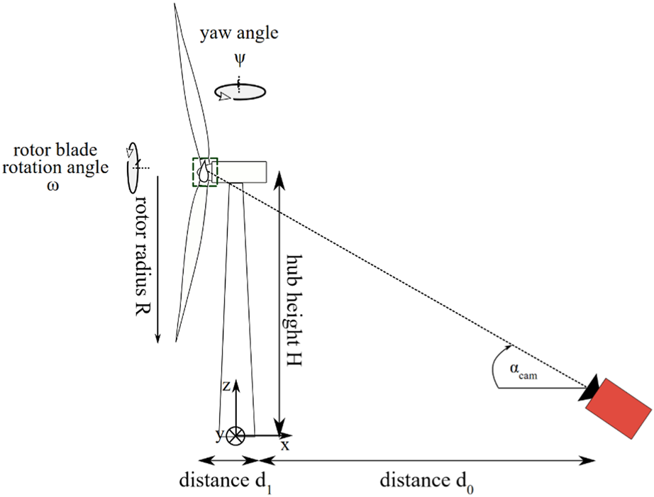
Side view of a wind turbine and the infrared camera, when the yaw angle is zero. The camera is pointed at a rotor blade with an elevation angle . The shown rotor blade position at is a special case, which is one of the two studied cases here. Note that the tilt angle of the rotation axis to the ground is neglected in the illustration.
Note that, similar to the distortion effect of the chord position, the radial position also differs from the measured position in the thermogram. To illustrate this effect, the measurement situation illustrated in side view in Figure 5 is additionally shown in top view in Figure 6. For a POI on the rotor blade surface, its radial position follows not only from the position in thermogram , but also from the blade geometry and the angle of view (compare with Eq. 1):
FIGURE 6

Top-down view of the wind turbine and the infrared camera introduced in Figure 1 for a negative yaw angle. A detailed top-down view of a rotor blade section is also shown. The azimuth angle of the camera is needed so that the camera is pointed towards the desired rotor blade section.
However, compared with the change of the geometry along the chord of the rotor blade, the change of the geometry along the radius is negligibly small. Therefore, the correction of the determined radial position will not improve our visualization of the boundary layer flow over the rotor blade. For this reason, the correction of the radius position is not considered here.
3 Experimental setup
3.1 Measurement object
The wind turbine, on which thermographic measurements are performed, is a 1.5 MW turbine from the manufacturer General Electric of the type GE 1.5sl located in Thedinghausen, Germany. Some of the wind turbine’s characteristics are summarized in Table 1. The 3d geometry of the blade, which is necessary for the geometric mapping algorithm, is here obtained by interpolating five laser line scans of an LM37P blade type of a 1.5 MW wind turbine described in Balaresque et al. (2016).
TABLE 1
| Hub height | 62 m |
| Rotor diameter | 77 m |
| Cut-in wind speed | 3 m/s |
| Rated wind speed | 15 m/s |
| Cut-out wind speed | 25 m/s |
Wind turbine GE 1.5sl characteristics.
The air temperature was around 19°C for the measurement and the weather was varying between sunny and cloudy, but without rain. No access to the wind turbine data existed. Therefore the wind speed was assessed with windfinder.com that yielded an average wind speed of about 5 m/s with gusts up to 9 m/s. During the actual measurement period, the wind speed is assumed to be constant, since the rotation frequency of the wind turbine was estimated to be constant at about 10 revolutions per minute. The latter was extractable from the time stamps of the measurement data for the blade passing events. The turbine is a pitch-controlled model, which up to a wind speed of 18 m/s controls the power output by changing the rotations per minute and above 18 m/s by changing the pitch angle of the rotor blades. Due to the weather conditions on the measurement day, i.e., low winds, a pitching of the rotor blades can be excluded from the geometrical considerations. A wind turbine yawing occurs when the wind direction changes.
3.2 Measurement setup
The measurement setup is shown in Figure 7, which consists of an IR camera to obtain thermographic images and a terrestrial laser scanner to obtain the yaw angle of the wind turbine. The camera and the laser scanner are placed with 1.5 m distance from each other downwind of the wind turbine, facing the suction side of the rotor blades.
FIGURE 7

Measurement setup. Left: Positioning of the infrared camera downwind of the wind turbine in operation. Right: Measurement system consisting of an infrared camera (left, red) and a terrestrial laser scanner (right, green) plus a battery as mobile power supply as well as one measurement laptop for each device.
The distance from the camera to the tower at the ground amounts to 127.8 m. To obtain IR images with a sufficient spatial resolution, a 200 mm telephoto lens is attached to the camera. As a result, not the entire blade but a rotor blade section of interest is imaged.
The adjusted camera view also sets the observed rotor blade position. According to
Figure 4, two different camera views are applied here to investigate the influence of the yawing on the thermographic flow visualization:
- The measurement position A is defined by the rotor blade being vertical to the ground at no yaw angle, pointing upwards (ω = 90°).
- The measurement position B is defined by the rotor blade being horizontal to the ground at no yaw angle, pointing left (ω = 180°).
At both blade positions, the influence of the blade cross-section according to the observed radial position r is considered. In particular, five different radial rotor positions r1 (close to the nacelle) to r5 (close to the tip) are observed, which are spaced by 17% of the rotor radius.
The terrestrial laser scanner is used in line-scanning mode, the scan line is aligned horizontally, and the angle of elevation amounts to 26.7°. Thus, the horizontal line through the nacelle is scanned, see dotted line in Figure 4. By evaluating the measured distances of passing rotor blades, the yaw angle is obtained.
A temporal synchronization of the yaw angle measurement and the thermographic measurement is realized by manually synchronizing the times of the two measurement laptops and evaluating the recorded time stamps. For the subsequent analysis, an assignment of both measurements to the same rotor revolution number is sufficient. If the desired temporal resolution is higher, an interpolation of the yaw angle measurement data would be required for the synchronization with the thermographic measurements at the position A.
3.2.1 Laser-based yaw angle measurement
In order to implement the geometric mapping algorithm, the yaw angle of the wind turbine has to be measured. Therefore a terrestrial laser scanner of the type LASE 2000D-228PLUS fromn the company LASE, is applied. The laser scanner’s relevant characteristics are summarized in Table 2. The laser scanner produces 1,000 measurement points over a 90° scan angle, and this scan line is repeated with a 30 Hz frequency.
TABLE 2
| Laser wave length | |
| Laser pulse rate | 40 kHz |
| Laser class | 1 M |
| Points per scan | 1,000 |
| Scan rate | 30 Hz |
Laser scanner LASE 200D-228PLUS characteristics.
The yaw angle of the wind turbine is extracted from the data acquired by the terrestrial laser scanner in horizontal scanning mode, which is pointed at the nacelle of the wind turbine at a certain elevation angle. From the data of each scan line, the rotor blades are extracted and the left and right rotor blade are distinguished using the prior knowledge about the position of the tower, which is visible in the scan data. The scan rate of the laser scanner is high enough that the same rotor blade is scanned multiple times during each revolution, but only the scan with the most data points is chosen to represent the blade and a threshold is applied concerning the minimum number of data points. This procedure is repeated for each of the three rotor blades and every revolution. Fitting a line through the points of each rotor blade and using the slope of the line together with the elevation angle, the yaw angle of the wind turbine is calculated. This results in a time-resolved measurement of the yaw angle, see Figure 8.
FIGURE 8

Yaw angle determined with the horizontally aligned laser measurement system for the detected rotor blades at the right (blue) and the left (orange) side of the nacelle. Data gaps occur, where the data amount from the laser scanner was too low to reliable detect a passing blade.
3.2.2 Thermographic flow visualization
For the thermographic measurements, the actively cooled infrared camera of the type imageIR 8300 from the manufacturer InfraTec is used. Important camera characteristics are listed in Table 3.
TABLE 3
| Frame rate | 100 Hz |
| Detector type | InSb (Indium antimonide) |
| Spectral range | 1.5 µm … 5.7 µm |
| maximum resolution | 640 pixels × 512 pixels |
| Integration time | 449 µs |
| Lens | 200 mm telephoto |
IR camera imageIR 8300 characteristics.
When the camera is orientated at a rotor blade section, it takes images with a frame rate of 100 Hz. However, a multitude of these images do not contain any parts of one of the three rotor blades. Therefore, the camera is instructed to save only those thermographic images that contain a rotor blade at a desired position. For this purpose, a respective temperature-threshold-based trigger is implemented by means of the camera control software Irbis Professional by InfraTec. By using this software, a rectangle is drawn in the live view of the camera output and a temperature condition is specified. As a result, the camera is triggered to save the current image when the temperature condition is fulfilled. As long as the trigger condition is fulfilled, the camera takes images with a frame rate of 100 Hz, resulting in multiple images of the rotor blade close to the desired blade recording position. In the post-processing, one image of each rotor blade pass per revolution, where the blade recording position is closest to the desired position, is chosen.
4 Analysis of the error correction potential
With the geometric mapping, the measured position of the POI in the thermographic image is converted to the associated relative chord position of the rotor blade. To clarify the necessity or the benefit of the geometric mapping, respectively, the corrected absolute measurement error of the relative chord position is studied. For this purpose, the geometric relations described in Section 2 are used to simulate the measurement conditions described in Section 3. The differencebetween the simulated measurement value with no geometric mapping and the true value of the relative chord position results in the systematic measurement error, which is corrected with the geometric mapping algorithm. This measurement error is calculated for the measurement locations A and B (see Figure 7), respectively, for different chord positions , and for five different radial rotor positions ranging from close to the nacelle () to close to the blade tip (). The with a.
First, the influence of the yaw angle on the measurement error is considered, which is shown in Figure 9 for different and for both measurement positions A and B. The radial position is (close to the nacelle). As expected for position A (see Section 2), the yaw angle has a significant influence on the error. The yaw angle and the error have an almost linear relationship, while the largest errors occur for = 0.3–0.4. The vanishing error of the curves for different at a yaw angle of approximately 12° is due to the pitch angle of the rotor blade. For yaw angles of ±, a position measurement error up to chord length occurs, which demonstrates the necessity for the error correction by means of the geometric mapping.
FIGURE 9

The difference over the yaw angle at the radius for different , for both rotor blade positions (A) (top) and (B) (bottom).
For position B, the uncorrected error has an offset and a non-linear, parabolic behaviour over the yaw angle, which is also in agreement with the theory derived in Section 2. The offset exists due to the oblique perspective on the rotor blade from the ground in addition to the blade surface tilt. As for position A, the maximal errors occur for = 0.3−0.4. For yaw angles between ±, the maximal measurement error amounts to chord length, which emphasizes the need for an error correction also for this measurement position.
As an example, the correctable measurement error for a yaw angle of and is shown over in Figures 10, 11, respectively, for different radii from close to the nacelle () to close to the tip (). As a result, the error shows a strong dependency on the relative chord position. Error peaks occur at a relative chord position of 0.3–0.4, where the blade thickness is maximal. Note that for position A the error is negative, while it is positive for position B. For blade position A, the error ranges from −9% to 0.5% and from −17% to 1%, respectively. This means the amplitude increases with the increasing yaw angle. For blade position B, the error ranges from 1% to about 7% for both yaw angle cases. The yaw angle influence is significantly lower at position B, which agrees with the theoretical predictions.
FIGURE 10

The difference over the relative chord length at the yaw angle for five different radii, and for both rotor blade positions A and B.
FIGURE 11

The difference over the relative chord length at the yaw angle for five different radii, and for both rotor blade positions A and B.
5 Results of a thermographic flow visualization with geometric mapping performed on an in-service yawing wind turbine
To verify the geometric mapping algorithm, a wind turbine rotor blade was equipped with aluminum markers, whose positions were known. The details of this setup are documented in Oehme et al. (2022a), Oehme et al. (2022b). The position of the markers was also determined in a picture of the rotor blades and subsequently fed into the geometric mapping algorithm, which calculates the chord position of the marker. As a result, the calculated chord position and the real chord position differs by only 2.3% of the chord length. Therefore, the geometric mapping algorithm is considered to be verified.
5.1 Results for position A
The expected error in localizing the chord position of a flow feature in the thermographic image, which occurs due the changing yaw angle of the wind turbine, is larger at the measurement position A. Therefore, the results for the measurement position A are discussed here.
Figure 12 shows single-shot thermograms that were captured during the yawing event, which is shown in Figure 8 at the time position 18 min. The three thermographic images from left to right show the thermographic measurement result for the last rotor revolution before the yawing, for the center yaw angle in the middle of the yawing, and for the first rotor revolution after the yawing motion of the turbine. The simultaneous laser measurement reveals a yaw angle change of 8°, from −32° to −40° (relative to the measurement position), compare with the respective yaw event shown in Figure 8.
FIGURE 12

Thermograms of a simultaneous measurement with the laser measurement system and the thermographic camera before, during and after the yawing of the wind turbine, which is shown in Figure 8 at the time 18 min. The leading and trailing edges as well as the position of the natural transition are each marked in sections to illustrate the optical displacement of the natural transition. In the raw thermograms, the position of the transition changes only by −0.4% with respect to the rotor blade width in the image.
At first, the detected chord position of the laminar-turbulent flow transition in the thermogram without any geometric mapping is determined, and the results are listed in the first row of Table 4. After feeding these values, together with the measured yaw angle, into the geometric mapping algorithm, the corrected chord positions result and are shown in the second row of Table 4. The uncorrected and corrected position values show three significant discrepancies.
TABLE 4
| Pre yawing (%) | During yawing (%) | Post yawing (%) | |
|---|---|---|---|
| No correction | 19.26 | 19.13 | 18.87 |
| With correction | 36.78 | 38.09 | 39.34 |
Chord position of the natural laminar-turbulent flow transition determined in the thermogram without any geometric mapping and after correction with the geometric mapping algorithm.
First, the mean position value is twice as large after the correction with the geometric mapping algorithm. The corrected error amounts to about 20% chord length, which is at least about one order of magnitude larger than the verified accuracy of the geometric mapping. This illustrates the significance of the studied error, when the camera perspective is not arranged perpendicular to the rotor blade chord. As a further evidence, that the corrected value of the transition position is close to the true value, thermograms from the measurement position B are studied, where the yaw angle influence is much lower or even negligible, see Section 2.2. For the measurement position B, the extracted transition position is at 38%, which is in excellent agreement with the obtained value at the measurement position A after correction.
Second, the uncorrected position values differ by only 0.4% for the considered yawing event. However, the position variation is considered to be a systematic effect, because the mean value of 100 position values along the radial blade axis is considered and, according to Dollinger et al (2018), the estimated position uncertainty for a single position value is in the order of 0.2%. After the correction, the magnitude of the detected position variation amounts to 2.5%, i.e., it is almost one order of magnitude larger. This qualitative behaviour and the order of magnitude is in very good agreement with former wind tunnel measurements, where the angle of attack was varied by −14° and the resulting shift of the transition position was 8%. The lower increase of the transition position during the yaw event at the wind turbine is plausible, because the relation between the inflow direction and the transition position is expected to be not linear and the change of the yaw angle is smaller.
Third and for the interpretation of the flow dynamics most important, the measured chord position decreases with no correction, while it is shown to actually increase when applying the geometric mapping algorithm. Indeed, a chord position increase is plausible, because the yawing was initiated due to a changed wind direction that meant a non-ideal angle of attack and, thus, a shift of the chord position of the laminar-turbulent flow transition to the leading edge. Therefore, the extent of the laminar flow region is expected to increase during and after the yawing. The thermographic imaging with geometric mapping shows the expected chord position increase of the flow transition.
As a result, the thermographic flow visualization needs to be combined with a (laser-based) yaw angle measurement and a geometric assignment to the 3d rotor blade surface, to enable an accurate analysis of the dynamic flow behavior on a yawing wind turbine.
6 Discussion and outlook
A 3d thermography system for the thermograhic flow visualization on wind turbine rotor blades was realized. For this purpose, a geometric mapping of the 2d image data onto the 3d rotor blade surface was used. While using a known turbine and blade geometry, the varying yaw angle of the wind turbine was measured with a laser scanner. This enables an accurate flow visualization during the wind turbine operation, in particular during the yawing of the rotor.
The chord position error of an identified flow feature in the thermogram depends on several quantities such as the true value of the chord position, the turbine and the blade geometry, the camera position in relation to the turbine position, the radial position of the observed rotor region, the rotation angle where the rotor is observed, and the yaw angle. The strongest impact of a varying yaw angle on the chord position error occurs for the vertical blade positions, and the lowest impact for the horizontal blade positions. Since the camera in general has a tilted view on the observed rotor blade region (because the camera is on the ground and the camera axis is not perpendicular to the rotor plane for zero yaw angle), the chord position error is typically non-zero, even for a zero yaw angle. For a varying yaw angle between ±30°, an absolute chord position error up to 17% and 7% occurs for a vertical and a horizontal blade position, respectively. Finally, the application of an error compensation with the geometric mapping was demonstrated for thermographic field measurements on a yawing wind turbine. As a result, the correct mean value of the chord position of the laminar-turbulent flow transition could be determined, and the previously hidden change of the transition position was resolved.
Thus, 3d thermography on yawing wind turbines is feasible. It enables a compensation of the disturbing influence of the varying camera perspective with respect to the rotor blade, e.g., during yawing but also during pitching and rotor rotation, so that an accurate localization of identified flow features on the 3d rotor blade surface is possible for in-service wind turbines. Note that this is relevant for evaluating measurements with a varying camera perspective (i.e., during yawing/pitiching/rotation) as well as for evaluating measurements with a static camera perspective difference.
Thus, while the present article is focused only on the yawing influence, the extended geometric mapping is a key element for future detailed flow studies at wind turbines in operation. For this purpose, a co-rotating measurement setup has been developed to continuously image a blade region of interest during the wind turbine motion, i.e., in particular during the rotor rotation and yawing. Most important, further field measurements on wind turbines are planned with the 3d thermography system to investigate the dynamic flow behavior of real operating wind turbines, in conjunction with the monitored turbine motion and the varying inflow and weather conditions.
Finally, future investigations should also focus on a complete uncertainty budget of the geometric mapping. For instance, the blade geometry is typically not exactly known, and the resulting uncertainty in the error correction needs to be clarified. The same holds for other parameters of the geometric model. However, in the worst case, if no blade geometry is available, a generic-type blade geometry can still be used as a first approximation to reduce the localization error.
Statements
Data availability statement
The raw data supporting the conclusion of this article will be made available by the authors, without undue reservation.
Author contributions
Conceptualization: AF and A-MP; Methodology: AF, A-MP, NB, and AvF; Software: A-MP and AF; Formal Analysis: A-MP, AF, NB, and AvF; Writing: A-MP and AF; Reviewing and Editing: AF, NB, and AvF. All authors contributed to the article and approved the submitted version.
Funding
This research was funded by Bundesministerium für Wirtschaft und Energie (BMWi) grant number 03EE3013.
Acknowledgments
The authors thank Felix Oehme and Daniel Gleichauf for their active support of the measurement campaign, for the helpful hints and discussions, and for providing the source code basis to enhance the geometric mapping to the 3d space.
Conflict of interest
Author NB was employed by Deutsche Windguard Engineering GmbH.
The remaining authors declare that the research was conducted in the absence of any commercial or financial relationships that could be construed as a potential conflict of interest.
Publisher’s note
All claims expressed in this article are solely those of the authors and do not necessarily represent those of their affiliated organizations, or those of the publisher, the editors and the reviewers. Any product that may be evaluated in this article, or claim that may be made by its manufacturer, is not guaranteed or endorsed by the publisher.
References
1
AptJ. (2007). The spectrum of power from wind turbines. J. Power Sources169 (2), 369–374. 10.1016/j.jpowsour.2007.02.077
2
BalaresqueN.BickerS.DollingerC.FandrichA.GatzS.HöllingM.et al (2016). Investigations for improvement of energy yield of rotor-blades from the 1.5 MW class. J. Phys. Conf. Ser.753 (7), 072012. 10.1088/1742-6596/753/7/072012
3
DollingerC.BalaresqueN.GaudernN.GleichaufD.SorgM.FischerA. (2019). IR thermographic flow visualization for the quantification of boundary layer flow disturbances due to the leading edge condition. Renew. Energy138, 709–721. 10.1016/j.renene.2019.01.116
4
DollingerC.BalaresqueN.SorgM.FischerA. (2018). IR thermographic visualization of flow separation in applications with low thermal contrast. Infrared Phys. Technol.88, 254–264. 10.1016/j.infrared.2017.12.001
5
DollingerC.SorgM.BalaresqueN.FischerA. (2018b). Measurement uncertainty of IR thermographic flow visualization measurements for transition detection on wind turbines in operation. Exp. Therm. Fluid Sci.97, 279–289. 10.1016/j.expthermflusci.2018.04.025
6
DoroshtnasirM.WorzewskiT.KrankenhagenR.RölligM. (2016). On‐site inspection of potential defects in wind turbine rotor blades with thermography. Wind energy19 (8), 1407–1422. 10.1002/we.1927
7
GalleguillosC.ZorrillaA.JimenezA.DiazL.MontianoÁ. L.BarrosoM.et al (2015). Thermographic non-destructive inspection of wind turbine blades using unmanned aerial systems. Plastics, Rubber Compos.44 (3), 98–103. 10.1179/1743289815y.0000000003
8
GleichaufD.DollingerC.BalaresqueN.GardnerA. D.SorgM.FischerA. (2020). Thermographic flow visualization by means of non-negative matrix factorization. Int. J. Heat Fluid Flow82, 108528. 10.1016/j.ijheatfluidflow.2019.108528
9
HwangS.AnY. K.SohnH. (2017). Continuous line laser thermography for damage imaging of rotating wind turbine blades. Procedia Eng.188, 225–232. 10.1016/j.proeng.2017.04.478
10
KuklovaJ.PopelkaL.SouckovaN.VituT. (2012). “Visualization of airfoil boundary layer by infrared thermography to determine influence of roughness-due-to-insect,” in Proceedings of the 11th International Conference on Quantitative InfraRed Thermography, Naples, Italy, June, 2012. 10.21611/qirt.2012.332
11
MedinaP.SchreckS.JohansenJ.FingershL. (2011). “Oil-flow visualization on a SWT-2.3-101 wind turbine,” in Proceedings of the 29th AIAA Applied Aerodynamics Conference, Honolulu, Hawali, June, 2011.3818.
12
OehmeF.GleichaufD.BalaresqueN.SorgM.FischerA. (2022b). Thermographic detection and localisation of unsteady flow separation on rotor blades of wind turbines. Front. Energy Res.10, 1043065. 10.3389/fenrg.2022.1043065
13
OehmeF.SorgM.FischerA. (2022a). Detection and localization of flow separation on wind turbines by means of unsteady thermographic flow visualization. J. Phys. Conf. Ser.2265 (2), 022101. 10.1088/1742-6596/2265/2/022101
14
ParreyA. M.GleichaufD.SorgM.FischerA. (2021). Automated detection of premature flow transitions on wind turbine blades using model-based algorithms. Appl. Sci.11 (18), 8700. 10.3390/app11188700
15
RaffelM.MerzC. B.SchwermerT.RichterK. (2015). Differential infrared thermography for boundary layer transition detection on pitching rotor blade models. Exp. Fluids56 (2), 30–13. 10.1007/s00348-015-1905-y
16
ReichsteinT.SchaffarczykA. P.DollingerC.BalaresqueN.SchüleinE.JauchC.et al (2019). Investigation of laminar-turbulent transition on a rotating wind turbine blade of multimegawatt class with thermography and microphone array. Energies12 (11), 2102. 10.3390/en12112102
17
TraphanD.HerráezI.MeinlschmidtP.SchlüterF.PeinkeJ.GülkerG. (2018). Remote surface damage detection on rotor blades of operating wind turbines by means of infrared thermography. Wind Energy Sci.3, 639–650. 10.5194/wes-3-639-2018
18
VeyS.LangH. M.NayeriC. N.PaschereitC. O.PechlivanoglouG.WeinzierlG. (2015). “Utility scale wind turbine yaw from a flow visualization view,” in Turbo Expo: Power for Land, Sea, and Air, Montreal, Quebec, Canada, June, 2015.
19
WaddleC. E.BolanJ. T.DobbinsC. L.HallZ. M.McDanielM. A. (2018). Visualization and analysis of boundary layer transitions using infrared thermography. Thermosense Therm. Infrared Appl. XL10661, 109–126. 10.1117/12.2304426
20
YuD. O.KwonO. J. (2014). Time-accurate aeroelastic simulations of a wind turbine in yaw and shear using a coupled CFD-CSD method. J. Phys. Conf. Ser.524 (1), 012046. 10.1088/1742-6596/524/1/012046
Summary
Keywords
infrared thermography, flow measurement, rotor blade geometry, yawing process, wind turbine dynamics
Citation
Fischer A, Parrey A-M, Balaresque N and von Freyberg A (2023) Flow visualization by means of 3D thermography on yawing wind turbines. Front. Energy Res. 11:1240183. doi: 10.3389/fenrg.2023.1240183
Received
14 June 2023
Accepted
23 October 2023
Published
08 November 2023
Volume
11 - 2023
Edited by
Stefano Leonardi, The University of Texas at Dallas, United States
Reviewed by
Umberto Ciri, University of Puerto Rico at Mayagüez, Puerto Rico
Yaqing Jin, The University of Texas at Dallas, United States
Updates
Copyright
© 2023 Fischer, Parrey, Balaresque and von Freyberg.
This is an open-access article distributed under the terms of the Creative Commons Attribution License (CC BY). The use, distribution or reproduction in other forums is permitted, provided the original author(s) and the copyright owner(s) are credited and that the original publication in this journal is cited, in accordance with accepted academic practice. No use, distribution or reproduction is permitted which does not comply with these terms.
*Correspondence: Andreas Fischer, andreas.fischer@bimaq.de
Disclaimer
All claims expressed in this article are solely those of the authors and do not necessarily represent those of their affiliated organizations, or those of the publisher, the editors and the reviewers. Any product that may be evaluated in this article or claim that may be made by its manufacturer is not guaranteed or endorsed by the publisher.