Voltage sag source location based on multi-layer perceptron and transfer learning

The existing voltage sag source localization only utilizes one simulation type or measurement data based on sampled waveform data. Moreover, it requires more storage space and transmission channels and cannot combine the advantages of simulated and measurement data, resulting in poor applicability of the model. Hence, this paper proposes a voltage sag source locating method based on transfer learning from the sag information in the sag event list combined with the grid structure data. Firstly, the location features of the sag source are extracted from the degree of sag impact, network structure, and sag-type information based on the characteristics of simulated and measurement data that characterize the position of the sag source, and they are collectively used as inputs to the model. Then, the simulated data is used to build a multi-classification model based on the multi-layer perceptron with the line number as the classification number, and the measurement data is employed to fine-tune the model parameters to achieve transfer learning. Finally, voltage sag source localization is achieved based on the trained multi-classification model. The correctness of the proposed method in this paper is verified through simulation and actual measurement in a specific area of East China.

1 Introduction

Voltage sag, being a critical power quality concern in the power system, has attracted the attention of both power supply and consumption parties (Hamdan, et al., 2020; Liu et al., 2020; Zhang et al., 2021; Jia et al., 2023). To understand the situation of power grid faults, quickly identify the sources of voltage sags, and provide targeted operation and maintenance to reduce the impact of voltage sags, it is necessary to conduct research on the localization of voltage sag sources (Meng et al., 2022). In addition to fault location, sag source localization uses the feature quantities measurement by monitoring devices to determine the approximate location of the sag source. Subsequently, it associates the grid side faults through the fault recording system to understand the affected range of users without monitoring devices and refine the affected area of users. Furthermore, it plays an important supporting role in enhancing inspection efficiency, helping users develop temporary power supply plans and defining the responsibility-sharing relationship between power supply companies and users during voltage sag events (Chen et al., 2019; Lv et al., 2021).

Since short-circuit faults are the most likely to occur and have the most extensive impact range, the voltage sag caused by short-circuit faults is also the most severe harm (Si et al., 2017). Therefore, the sag source location is generally studied for grid-side faults. Recently, a large amount of research has been conducted on identifying the sag source location both domestically and internationally. Traditional sag source localization methods mainly rely on physical feature quantities to determine whether the voltage sag source is located upstream or downstream of the monitoring point. According to the different selected feature quantities, traditional methods are mainly divided into two categories: disturbance power and energy methods (Parsons et al., 2000) and parameter transformation methods (Mohammadi et al., 2017; Tang et al., 2017). The former defines the relative position of the voltage sag in the monitoring device based on the energy flow direction. The latter determines whether the voltage sag source is located upstream or downstream of the monitoring device based on the changes in system parameters before and after the fault. Thus, Lv et al. (2019) regarded upstream and downstream locations as a binary classification problem and combined multiple localization features to improve the upstream and downstream localization accuracy. It should be noted that the mentioned approaches can only define the responsibility-sharing relationship between users and grid companies, while they are not able to refine the impact of different line faults on users and cannot provide temporary power supply plans and decision-making support for users. To narrow the search range for sag sources, Hu et al. (2021) proposed a voltage sag source localization method in distribution networks based on wavelet energy entropy, relying on the sensitivity of wavelet energy entropy to sudden changes in signals. While this method reduced the location results to the nearest node to the sag source, certain limitations arose when dealing with nodes that have many branches. With the deepening of research, locating the specific location of the sag source has become a hot research topic. This type of research is mainly based on two types of methods: signal processing and deep neural networks. Regarding signal processing, Yang et al. (2022) processed voltage and current signals during faults, employed neural networks to determine candidate regions for voltage sag, and achieved precise localization of sag sources through moths to the fire optimization algorithm. Lu et al. (2020) utilized the voltage and current information recorded by Supervisory Control and Data Acquisition (SCADA) for fault line selection. They also employed the simplified R-L model’s dual terminal positioning method to achieve the precise location of the sag source. However, this type of method did not consider the varying degrees of changes in actual power grid parameters with environmental conditions, load conditions, and other conditions, resulting in inaccurate sag localization results. In terms of deep neural networks, Deng et al. (2021) took the measurement voltage waveform at monitoring points as input and used an independent recurrent neural network of attention to achieve voltage sag source localization. Nevertheless, this method relied on a large amount of high-quality measurement data. However, the data and quality of actual monitoring data were difficult to ensure training requirements, which made this method have certain limitations.

Based on the above analysis, it can be inferred that the existing methods for locating voltage sag sources are all based on sampled value data of voltage and current waveforms, which requires more storage space and transmission channels. Moreover, the data is prone to loss during transmission and conversion processes. On the other hand, the above methods are based on simulation analysis or driven by measurement data, both of which have certain limitations. The simulation-based analysis method is only an approximation of real power grid faults due to the inability to restore the fault mechanism accurately and actual influencing factors, making it difficult to guarantee that it is also applicable to measurement data. The method driven by measurement data faces limitations in terms of the number of monitoring points, resulting in a small number of measurement samples, uneven distribution of data, and difficulty in ensuring the quality of measurement data (Huang et al., 2022). These factors result in insufficient model training and affect positioning accuracy.

Currently, no literature research exists on combining simulated and measurement data for realizing the sag source location. Therefore, this paper proposes a voltage sag source localization method based on transfer learning from sag information in the sag event list, relying on simulation and measurement data characteristics. The main contributions of this paper are presented as follows.

1) This proposed method has a low configuration for monitoring terminals, and the data can be obtained from the list of sag events, which is convenient and simple to obtain. In the future, it can be integrated as a functional module into relevant systems, such as voltage sag monitoring systems, to achieve real-time positioning, and has high engineering practical value.

2) This paper incorporates the common attributes of simulated and measurement data, uses simulation data for pre-training, and freezes some parameters. Then, it employs measurement data for correction, realizing the complementarity of two data types under the transfer learning mechanism and making up for the lack of small sample data and uneven distribution.

3) The proposed method is validated using actual monitoring and simulation data from the East China region. The best-frozen layer is obtained by freezing the parameters of different layers of the multi-layer perceptron. In addition, this article also compares the proposed method with other pre-training methods.

The remaining sections of this paper are organized as follows: Section 2 elaborates on the basic knowledge of voltage sag source localization. In Section 3, the acquisition methods and data characteristics of simulated and measurement data are presented. Thus, voltage sag source location features are introduced from the multi-dimensional perspectives of sag impact degree, network structure, and fault type information. Section 4 introduces the multi-layer perceptron and transfer learning mechanism and describes the process of the proposed voltage sag source localization method. In Section 5, the applicability of the multi-layer perceptron in this paper is first verified. Subsequently, the feasibility of the proposed method is validated using the simulation and measurement data of a region in East China. Finally, conclusions are drawn in Section 6.

2 Preliminaries on voltage sag source location

The increase in system current is the reason for the voltage sag caused by a short circuit fault, which leads to a reduction in the voltage of nearby nodes. Equivalent model of voltage sag caused by short circuits established in literature (Hu et al., 2021) is shown in Figure 1, and the voltage amplitude calculation at the common connection point is summarized in Eqs. 1–3.

FIGURE 1

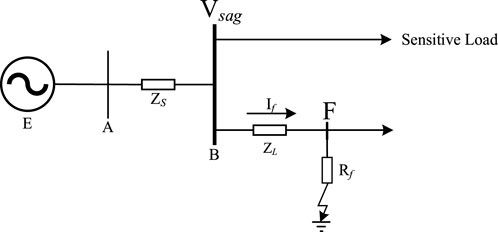
FIGURE 1. Equivalent model of voltage sag caused by short circuit.

In Figure 1, E represents the grid voltage, Z_L denotes the line impedance between the fault point and node B, Z_S indicates the line impedance between transmission line AB, F shows the fault location, R_f defines the transition impedance. Moreover, I_f is the fault current, which can be calculated by the following equation.

${\mathbf{I}}_{\mathit{f}}=\frac{\mathit{E}}{{\mathit{Z}}_{\mathit{S}}+{\mathit{Z}}_{\mathit{L}}{+\mathit{R}}_{\mathit{f}}}(1)$

The voltage amplitude Vsag of node B is:

${\mathit{V}}_{\mathit{s}\mathit{a}\mathit{g}}=\frac{\left({\mathit{Z}}_{\mathit{S}}{+\mathit{R}}_{\mathit{f}}\right)\ast \mathit{E}}{{\mathit{Z}}_{\mathit{S}}+{\mathit{Z}}_{\mathit{L}}{+\mathit{R}}_{\mathit{f}}}(2)$

Assuming the grid voltage E = 1, the line satisfies a uniform distribution, in which the impedance per unit length of the line is z, and the total line length is l. Therefore, Eq. 2 can be re-written as follows:

${\mathit{V}}_{\mathit{s}\mathit{a}\mathit{g}}=\frac{\mathit{z}\ast \mathit{l}{+\mathit{R}}_{\mathit{f}}}{{\mathit{Z}}_{\mathit{S}}+{\mathit{Z}}_{\mathit{L}}{+\mathit{R}}_{\mathit{f}}}(3)$

The above equation shows that the amplitude of node voltage is related to the fault location, transition resistance, and fault type. Specifically, the amplitude of node voltage exhibits a gradual increase with distance from the fault point, indicating that the impact diminishes as one moves farther away from the fault point. Moreover, the amplitude of node voltage gradually rises with the increase of transition resistance. Furthermore, the amplitude of node voltage is also affected by the type of fault, and different types of faults result in different ranges of voltage sags, with three-phase faults having the most extensive influence. In addition, changes in the power grid structure can lead to varying degrees of electrical distance between faulty nodes and each node, thereby affecting the voltage amplitude at those nodes. Therefore, voltage sag can be seen as the result of the joint action of faults and the power grid structure. Suppose the power grid structure remains unchanged when the same fault type occurs on the same line. In that case, the affected nodes are roughly the same, and the voltage sag amplitude changes of each affected node have a certain degree of similarity. The voltage amplitude and fault type of the affected nodes can also describe and determine the impact range of a voltage sag event under the power grid structure. However, it is difficult to obtain the voltage amplitude information of each node in the entire network in practice. Moreover, monitoring node recording of sag information can also reflect the sag situation of the entire network to a certain extent. In conclusion, the location information of sag sources can be mined by examining the voltage amplitude, fault type, and power grid structure of the disturbed monitoring points.

3 Data source and feature selection

This section is mainly divided into two parts: the first part introduces the characteristics and acquisition methods of simulation and measurement data; The second part selects voltage sag source localization features from different perspectives to characterize the position of the sag source and provides corresponding calculation formulas.

3.1 Data source

This paper considers simulated and measurement data characteristics and uses them as data support for locating voltage sag sources. It compensates for the shortage of small samples in measurement data and considers factors such as actual load conditions and changes in grid structure at the simulation level. Therefore, data acquisition can mainly be divided into two aspects, including simulated and measurement data.

3.1.1 Simulated data

The voltage sag simulation data is derived from the Engineering Production Management System (PMS2.0), which obtains the parameters of power grid equipment system components, including line and transformer parameters for power grid modeling and simulates and calculates different lines and fault scenarios within the entire network. The voltage amplitude data of each node is obtained, and the simulation results, such as voltage amplitude, fault type, and power grid operation mode of each node, are used as the source of simulation data.

This paper selects Bonneville Power Administration (BPA) as a simulation calculation tool, mainly by constructing data cards, such as B card, L card, and T card, for power components to achieve large-scale simulation calculation of power systems. This approach has the advantages of simple operation and accurate calculation results (Wang et al., 2021). The simulation process entails selecting random variables, namely, fault lines, fault distances, fault types, fault phases, and fault duration, in BPA to simulate the randomness of grid side faults.

Since fault simulation calculations are based on physical models and fault differential equations, this data type includes the mechanism of the transient simulation model, reflecting the voltage sag situation under different fault scenarios and operating modes. However, it is important to note that the impact of factors, such as load conditions, in the actual environment on the transient level.

3.1.2 Measurement data

The measurement data sources of existing sag locating methods rely on all waveform data of voltage or current sampling values recorded by fault recording systems, which require more storage space and transmission channels. Moreover, transmission and conversion processes may result in the loss of sampling values, thereby affecting positioning accuracy. In contrast, the list of sag events includes information, such as monitoring point sag amplitude, fault type, sag occurrence time, and duration, which has the advantages of easy access and high real-time performance (Huang et al., 2022). Therefore, this study selects the list of sag events as data support. However, it is important to note that the triggering time and duration of a single voltage sag event are random, and their numerical values are influenced by external environmental factors, such as protection action time, which cannot reflect the location information of the sag source. To address this limitation, the monitoring point sag amplitude, sag type, and power grid structure data in the dispatching system included in the list of sag events are collectively used as the source of the measurement data. This type of data compensates for the shortcomings of simulation data from a practical perspective. However, the availability of monitoring devices for power grid sag is currently limited, resulting in a small sample size and uneven distribution of various sag events.

3.2 Feature selection

To achieve sag location of small sample measurement data, this paper combines the advantages of large simulation data volume and complete measurement data information. Then, based on the simulation and measurement data sources in Section 3.1, voltage sag source location features are selected from different perspectives to characterize the position of sag sources, as listed in Table 1. Through the introduction of transfer learning, pre-training is carried out with the help of simulation data. Then, the measurement data is used to fine-tune the model parameters to achieve sag positioning.

1) Information of The Degree of Impact of Voltage Sag

TABLE 1

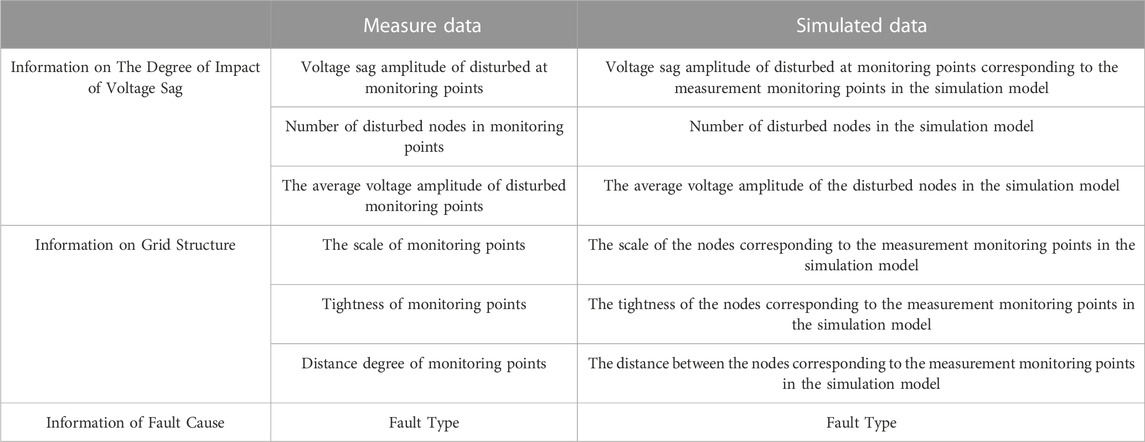
TABLE 1. Locating features of voltage sag source.

The impact degree of voltage sag can characterize the physical properties of the power grid to some extent, specifically highlighting how the transmission of voltage sag is affected by distance and exhibits attenuation characteristics. The impact range and severity of a single voltage sag event are described using the information on sag impact degree. To provide a clear definition, the node where the monitoring point records the amplitude of the sag is used as the disturbed node in actual systems. Conversely, a sag amplitude below 0.9 in the simulation model is considered a disturbed node.

The calculation formula for the sag amplitude in disturbed voltage at the monitoring point is as follows:

$\mathit{X}=\mathit{U}°\mathit{D}(4)$

where $°$ represents the multiplication of the corresponding elements of matrix U and D, U indicates the voltage sag amplitude of each monitoring node during a certain sag event, and D denotes the disturbance status of each monitoring node, with disturbance being 1 and undisturbed being 0. The values of sag amplitude in the simulation and actual measurement systems are as follows: In the actual system: if the monitoring point records this voltage sag event, the monitoring point is affected by this voltage sag event, and the sag value is the recorded value. On the contrary, if the monitoring point is unaffected, the sag amplitude is 1. In the simulation system: the voltage amplitude is the simulation calculation result.

Since the list of sag events only contains information about the disturbed monitoring nodes, and the simulation results encompass information about each node within the entire network, the benefit of the simulation calculation results, including all node information, is described using the number of disturbed monitoring nodes N (NM: measurement system, NS: simulation system) and the average voltage sag amplitude E of the disturbed nodes. The calculation formula is shown in Eqs. 5–7:

${\mathit{N}}_{\mathit{M}}={\displaystyle \sum _{\mathit{i}\in \mathit{M}}}\mathbf{n}\mathbf{u}\mathbf{m}\left({\mathit{b}}_{\mathit{i}}\right)(5)$

${\mathit{N}}_{\mathit{S}}={\displaystyle \sum _{\mathit{j}\in \mathit{B}}}\mathbf{n}\mathbf{u}\mathbf{m}\left({\mathit{b}}_{\mathit{j}}\right)(6)$

where M represents the set of monitoring points, B indicates the set of all nodes in the simulation system, b denotes the disturbed node, and num (·) is the calculated quantity.

The calculation formula for the average voltage drop amplitude E is as follows:

$\mathit{E}=\frac{\mathbf{s}\mathbf{u}\mathbf{m}\left(\mathit{X}\right)}{\mathit{N}}(7)$

where sum (·) represents the sum of matrix elements.

2) Information of Grid Structure

The information pertaining to the impact degree of voltage sags only characterizes the degree of impact based on the physical properties of the power grid, thereby lacking the ability to characterize the level of impact from the perspective of topological properties (the power grid structure). Conversely, the actual power grid undergoes changes in operating conditions and line maintenance, causing changes in the interconnection between nodes and altering the propagation path of voltage sags. Therefore, this study takes the simulation model of the power grid structure as the benchmark to depict the changes in the actual power grid structure. Moreover, it introduces the scale degree F_i, tightness degree C_i, and distance degree L_i of monitoring points to describe the information of power grid structure based on Hu et al. (2020). The calculation formula is as shown in Eqs. 8–10.

The node susceptibility to voltage sags directly increases when the node is connected to more lines, reflecting the node’s direct impact ability. Conversely, when fewer lines are connected to a node, more lines are connected to adjacent nodes. Thus, the node is still susceptible to voltage sags, demonstrating the node’s indirect impact ability. Therefore, considering the interconnection between nodes and adjacent nodes, the scale of monitoring points is defined as F_i, describing the difficulty degree of monitoring points affected by voltage sags. The calculation formula for F_i is as follows:

${\mathit{F}}_{\mathit{i}}={\mathit{f}}_{\mathit{i}}+{\displaystyle \sum _{j\in G}}{\mathit{f}}_{\mathit{j}}(8)$

where f_i represents the number of adjacent nodes at monitoring point i, and G indicates the set of adjacent nodes at monitoring point i.

Since the scale of monitoring points, F_i, only defines the scale of nodes and adjacent nodes, the impact of voltage sag transmission paths is not considered. Therefore, the monitoring node tightness C_i describes the degree of impact of voltage sag on monitoring points through various paths. The calculation formula is as follows:

${\mathit{C}}_{\mathit{i}}=\frac{\mathbf{2}{\mathit{c}}_{\mathit{i}}}{{\mathit{n}}_{\mathit{i}}\left({\mathit{n}}_{\mathit{i}}-\mathbf{1}\right)}(9)$

where c_i represents the monitoring point i and the number of adjacent node lines, and n_i denotes the number of adjacent nodes of monitoring point i. In theory, as n_i adjacent nodes can generate (n_i −1)n_i/2 lines, C_i can represent the tightness of node i.

Owing to changes in operating conditions and line maintenance in the actual power grid, the connection mode between nodes undergo alterations, further influencing the severity of voltage sag events at monitoring points. Hence, this paper defines the degree of distance L_i to describe the impact of changing branches on monitoring points. Assuming the endpoints of the changing branch are j and k, the calculation formula is as follows:

${\mathit{L}}_{\mathit{i}}=\mathbf{min}\left\{{\mathit{l}}_{\mathit{i}\mathit{j}},{\mathit{l}}_{\mathit{i}\mathit{k}}\right\}(10)$

where l_ij represents the shortest electrical distance between the monitoring point i and the endpoint j of the branch where the distance changes, and l_ik symbolizes the shortest electrical distance between the monitoring point i and the endpoint k of the change branch.

3) Information of Fault Type

As the information on the degree of impact of voltage sags and the power grid structure only characterize the external characteristics of voltage sags, the influence of internal characteristic factors is ignored. Since the impact range of voltage sags caused by different fault types is different, the voltage sags caused by three-phase faults have the most severe impact. Therefore, fault type T is selected in this paper to represent the fault cause information.

To facilitate the input of subsequent models, different fault types are represented by numerical values of T = 1, 2, 3, and 4, corresponding to single-phase grounding, interphase short circuit, two-phase grounding, and three-phase short circuit, respectively.

4 Method for identifying the location voltage sag sources

This section introduces the principle and structure of multi-layer perceptron (MLP). Then, it introduces the transfer learning mechanism and finally introduces the process of voltage sag source location based on transfer learning.

4.1 Multilayer perceptrons

Regarding the results of sag source location, there are two aspects to consider. Firstly, upstream and downstream locations can only divide the responsibility sharing relationship between users and the power grid company. Although identifying a specific location can address the location needs, it has certain shortcomings, such as large computational complexity resulting from multivariate optimization solutions. Secondly, the power grid company aims to associate grid-side faults through fault recording systems and understand the situation of line faults to improve targeted operation and maintenance efficiency. It is worth noting that enterprise users pay more attention to the relative location of the sag source to provide a basis for subsequent economic disputes. They also focus on the impact area of line faults to assist in formulating resumption of work and production plans rather than focusing on the specific location of the sag source. Therefore, the sag source location needs of the power grid layer and the user layer are taken into account, and the result of the sag location is determined as the line where the sag source is situated. Under the assumption of an unchanged power grid operation mode, when the same type of fault occurs on the same line, and the selected features in Section 3.2 exhibit a certain degree of similarity, voltage sag source location can be defined as a multi-classification problem. Moreover, the classification number can be determined based on the number of lines as the classification result. Therefore, there is a need for an effective algorithm to solve multi-classification problems.

MLP is a feedforward neural network composed of input, hidden layer, and output layers in which a full connection mode is adopted between layers (Zhang et al., 2022). As the single-layer perceptron cannot be separated from nonlinear data, MLP introduces a hidden layer to overcome this defect because the multi-layer perceptron can better solve the multi-classification problem (Zhang et al., 2022). Hence, MLP is selected as the multi-classification algorithm for identifying voltage sag source location. The structural schematic diagram is shown in Figure 2. The whole implementation process of MLP is summarized in Eqs. (11)–(13) (Zhang et al., 2022).

FIGURE 2

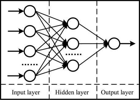
FIGURE 2. Schematic diagram of multi-layer perceptron structure.

Assuming the input as $X=\left[x_1,x_2,\cdots ,x_n\right]$, the number of neurons in the hidden layer is m, and the mapping relationship from the input layer to the hidden layer can be determined as follows:

$\mathit{H}=\mathit{f}\left({\mathit{W}}_{\mathbf{1}}\ast \mathit{X}+{\mathit{B}}_{\mathbf{1}}\right)(11)$

where f () represents the activation function of the hidden layer, W1 indicates the n*m dimensional matrix, and B₁ denotes the m*1 dimensional matrix.

The mapping relationship from the hidden layer to the output layer is as follows:

$\mathit{H}=\mathit{g}\left({\mathit{W}}_{\mathbf{2}}\ast \mathit{H}+{\mathit{B}}_{\mathbf{2}}\right)(12)$

where g() represents the activation function of the hidden layer, W₂ demonstrates the m*1 dimensional matrix, and B₁ denotes the m*1 dimensional matrix.

The final classification result is affected by the mentioned number of hidden layer neurons. If the number of hidden layer neurons is too small, it will be challenging to accurately fulfill the learning and classification requirements. In contrast, when the number of neurons in the hidden layer is too large, it is easy to create overfitting, thereby resulting in poor generalization ability of the network. The number of hidden layer neurons can be determined using Eq. 13.

$\mathit{d}=\lceil \sqrt{\mathit{p}+\mathit{q}}+\mathit{a}\rceil (13)$

where $\lceil \rceil$ represents rounding up, p indicates the dimension of the input layer parameter matrix, and q denotes the number of multiple classifications. Moreover, a indicates the adjustable constant of [1,10] to ensure the model’s adaptability, and d symbolizes the number of neurons in the hidden layer.

4.2 Transfer learning

The small amount of measurement data may lead to insufficient model training, which may affect the accuracy of the sag source location. Thus, this paper introduces the transfer learning mechanism to train the measurement data, considering the advantages of easy access to simulation data and large amounts of data.

Transfer learning is a machine learning idea suitable for new tasks or functions by fine-tuning existing models (Hopson et al., 2023). In transfer learning, the learning domain containing many label data is called the source domain, and the learning domain with fewer label data is called the target domain. The model is pre-trained using the data from the source domain and then fine-tuned through the target domain data to make full use of the source domain data to improve the model’s accuracy in the target domain. The calculation formula of transfer learning is summarized in Eqs. 14–17 (Hopson et al., 2023).

${\mathit{P}}_{\mathit{S}}={\mathit{f}}_{\mathit{S}}\left({\mathit{X}}_{\mathit{S}},{\mathit{\theta }}_{\mathit{S}}\right)(14)$

${\mathit{P}}_{\mathit{M}}={\mathit{f}}_{\mathit{M}}\left({\mathit{X}}_{\mathit{M}},{\mathit{\theta }}_{\mathit{M}}\right)(15)$

where ${\theta }_S$ and ${\theta }_M$ indicate parameters in the source domain and target domain, respectively. In addition, $X_S$ and $X_M$ represent datasets in the source and target domains, respectively. Furthermore, $f_S$ and $f_M$ are respectively the mapping relationship between the source domain and the target domain, and $P_S$ and $P_M$ denote the predicted values of the source and target domains, respectively. To minimize the error between the predicted value and the actual value labels, the objective function is set as follows:

${{\mathit{\theta }}_{\mathit{S}}}^{*}=\mathit{arg}\underset{{\mathit{\theta }}_{\mathit{S}}}{\mathbf{min}}\frac{\mathbf{1}}{{\mathit{N}}_{\mathit{S}}}{\displaystyle \sum _{\mathit{i}=\mathbf{1}}^{{\mathit{N}}_{\mathit{S}}}}\mathit{L}\left({\mathit{y}}_{\mathit{s}\mathit{i}},{\mathit{P}}_{\mathit{S}\mathit{i}}\right)(16)$

${{\mathit{\theta }}_{\mathit{M}}}^{*}=\mathit{arg}\underset{{\mathit{\theta }}_{\mathit{M}}}{\mathbf{min}}\frac{\mathbf{1}}{{\mathit{N}}_{\mathit{M}}}{\displaystyle \sum _{\mathit{i}=\mathbf{1}}^{{\mathit{N}}_{\mathit{M}}}}\mathit{L}\left({\mathit{y}}_{\mathit{M}\mathit{i}},{\mathit{P}}_{\mathit{M}\mathit{i}}\right)(17)$

where y_S and y_M are the true labels of the source and target domains, respectively. Moreover, N_S and N_M represent the number of training samples in the source domain and target domains, respectively, and L() denotes the loss function.

Since the simulation data in this paper is calculated based on physical models and fault differential equations and is influenced by objective factors in the real environment, i.e., weather and load conditions, it is difficult to ensure that the simulation and measurement data meet the same distribution. Considering the similarity between simulation and measurement data, the advantage of simulation data will be utilized to locate the voltage sag source of small sample data. The migration process follows the subsequent steps: Firstly, a multi-classification model is pre-trained using simulation data. Then, the parts of the multi-classification model requiring retaining are determined. Given the higher number of layers in the neural network, the more obvious the extracted features are, which means that the information in the previous layers is more general (Yang et al., 2022). Therefore, this paper aims to fix the parameters of the hidden layer only for fine-tuning, while retaining the output layer parameters. Finally, a multi-classification model that can accurately locate small sample data from actual measurements is obtained. Figure 3 illustrates the model.

FIGURE 3

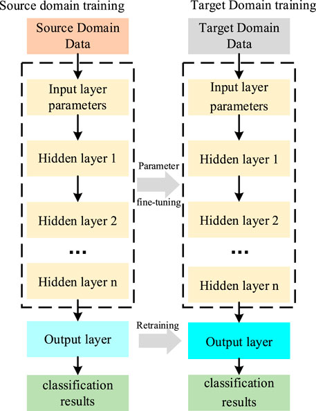
FIGURE 3. Schematic diagram of Transfer learning structure.

4.3 Positioning process

Figure 4 depicts the flow chart of the proposed voltage sag source localization method based on transfer learning. The specific process is outlined as follows: Firstly, using the information provided in Section 3.1, the simulation dataset (MS) and the measurement dataset (MM) are obtained. The calculation formulas presented in Section 3.2 for determining the degree of sag impact, grid structure, and sag type information are then employed to construct a feature matrix for both obtained simulation and measurement datasets. Secondly, a multi-classification model based on a multi-layer perceptron is constructed, with the fault line number serving as the classification number. The model is pre-trained using the feature matrix derived from the simulation dataset. Next, some model parameters are frozen, and the model is trained using the characteristic matrix formed by the measurement dataset to achieve transfer learning. Finally, test set samples are input into the final multi-classification model to achieve voltage sag source location.

FIGURE 4

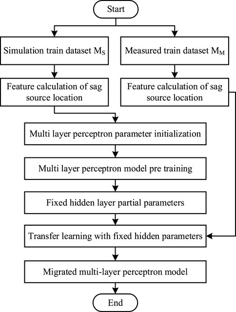
FIGURE 4. Flow of voltage sag source location based on multi-layer perceptron and Transfer learning.

5 Example analysis

To verify the applicability of the proposed method in practice, a selection of sag information from a certain region of East China, recorded in the list of sag events between January 2019 to May 2021, is utilized. This area contains 25 lines, with voltage levels including 220, 110, and 10 kV. The actual network includes four transformers, consisting of 1 Ynyn and 3 Ynd11. Additionally, 6 power quality monitoring terminals are installed. The structural diagram is shown in Figure 5. During this period, a total of 62 sag events have been recorded in the list of events. In this study, the amplitude and fault type of the sag events are chosen, and the network structure information is retrieved from the scheduling system as the measurement data source, forming 54 sets of data.

FIGURE 5

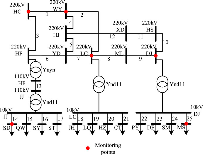
FIGURE 5. Actual line structure of a certain area in East China.

The dataset consisting of 54 sets of data is divided into training and testing sets for further analysis. The process involves randomly selecting 36 pieces of data as the testing set, while the remaining 18 pieces of data are designated as the training set. Table 2 provides the frequency distribution of training and testing sets under different fault types.

TABLE 2

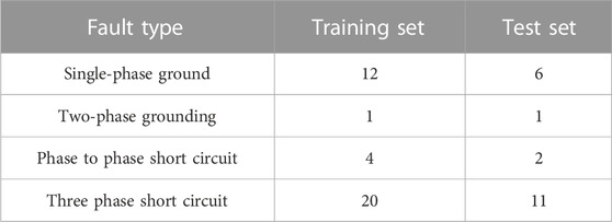
TABLE 2. Actual data training set and test set data.

Using the Engineering Production Management System (PMS2.0), component parameter data for the power grid equipment system (including line, transformer parameters, etc.) is obtained. Based on this data, a BPA simulation model is built for a specific area in East China, as shown in Figure 5. To accurately simulate the randomness of voltage sag, fault lines, fault distance, transition resistance, fault type, and duration are selected as random variables, and 1,200 sets of data are obtained through model simulation. Table 3 presents the distribution of simulation times under different fault types.

TABLE 3

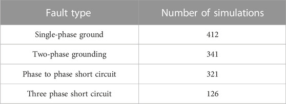
TABLE 3. Various fault settings in the simulation model.

MLP parameters are set as follows: weight optimization method solver = 'adam' (lr = 0.001, betaz_1 = 0.9, betaz_2 = 0.98, epsilon = 1e-8); activation = “relu”; loss = [“categorical_crossentropy,” “mae”]; Alpha = 1e-5; epochs = 1,000; hidden layers are set to 4, and the number of neurons per layer is set to m = 35; the number of neurons in the output layer is set to 25. Moreover, accuracy is chosen as a comparative indicator. The calculation formula for accuracy is as follows:

$\mathit{A}\mathit{c}\mathit{c}\mathit{u}\mathit{r}\mathit{a}\mathit{c}\mathit{y}=\frac{{\mathit{C}}_{\mathit{N}}}{{\mathit{T}}_{\mathit{N}}}\times \mathbf{100}\%(18)$

where T_N represents the total number of samples, and C_N denotes the number of correctly classified samples.

The proposed method involves pre-training MLP using simulation data. Following this, different hidden layer parameters are frozen, and then the model is trained again using measurement data. When retraining, parameters are set to: solver = “adam” (lr = 0.005, betaz_1 = 0.9, betaz_2 = 0.98, epsilon = 1e-7); loss = [“categorical_crossentropy,” “mse”; Alpha = 1e-5; epochs = 1,000. Hidden layers are set to 4, and the number of neurons per layer is set to m = 35; the number of neurons in the output layer is set to 25. The classification accuracy of different fault types is calculated using Eq. 18, as shown in Figure 6.

FIGURE 6

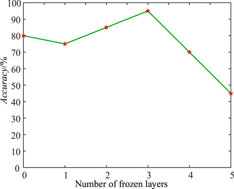
FIGURE 6. Accuracy of freezing different layers.

As can be seen in Figure 6, the model is retrained using measurement data after pre-training the multi-classification model with simulation data, as the number of frozen layers is 0. Due to the lack of frozen hidden layer parameters, it is equivalent to only using measurement data to train the model. However, when the number of measurement samples is relatively small and the distribution of different types of transient events is uneven, the accuracy of the actual test set is not very high. On the other hand, when only the first layer parameters are frozen, and the model is retrained using measurement data, the model’s adaptability is affected to a certain extent. This impact is due to the addition of parameters obtained from simulation data training, which decreases the accuracy of the measurement test set samples. As the number of hidden layers increases, the model’s ability to extract features will be strengthened. Therefore, more frozen layers enhance the model’s ability to extract common features from simulated and measurement data. However, certain differences exist between simulation and measurement data when the number of frozen layers reaches a certain level because the obtained parameters from the simulation training model are greater than those obtained from the measurement training model, leading to a gradual decrease in the accuracy of the measurement test samples. Therefore, when the entire model is frozen, the accuracy is the lowest due to relying only on the parameters obtained from simulation training. Thus, it can be observed from the figure that the optimal number of frozen layers is 3. Accordingly, after training the model using simulation data, the hidden layer parameters are frozen and used as universal parameters. Subsequently, the model is retrained using measurement data, and the parameters of the other layers are adjusted.

In this section, To verify the effectiveness of the proposed algorithm in this section, a comparative analysis is conducted with the other two types of training methods. Method 2 only uses measured data for model training, while Method 3 utilizes a combination of simulation and measured data. The loss curves of the three types of training methods are shown in Figure 7, and the accuracy rates under different training methods are calculated using Eq. 18, as shown in Table 4.

FIGURE 7

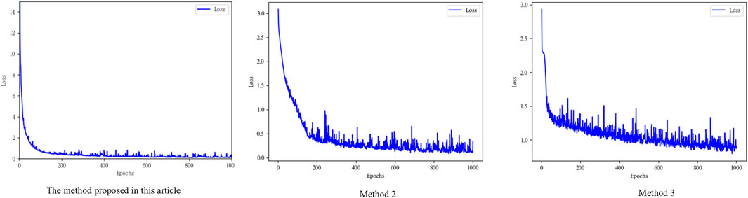
FIGURE 7. Loss curves of different training methods.

TABLE 4

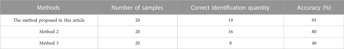
TABLE 4. Comparison of accuracy results of different training methods.

As seen in Figure 7, since there is a certain degree of similarity between the simulation and the measured data, this paper first uses the simulation data for pre-training, which speeds up the convergence rate of the measured data re-training. Furthermore, it overcomes the overfitting problem caused by the small sample of the measured data. The specific performance is as follows: The loss curve declines sharply at first due to the training method adopted in this paper. After 130 iterations of training, the Loss function value tends to be stable. When the training is completed, the Loss function value reaches 0.0836. These training results indicate that the network converges, and the fitting effect are acceptable.

Conversely, the model cannot well fit the real distribution of data for the training method adopted in Method 2 due to the small amount of measured data, resulting in the poor generalization ability of the model. In addition, despite 130 training iterations, the Loss function curve tends to be stable but at a high level (loss value exceeding 0.2), indicating the inability to reach a lower loss. For Method 3, since the training samples contain both simulation and measured data, the distribution of the two data types is very different, leading the model to switch back and forth between the two types of data and oscillation of the Loss function curve. Consequently, after 1,000 iterations, the loss function value fails to exhibit a stable trend. In addition, the model will be easier to learn the simulation data because the two data types have a large difference in the characteristic distribution. However, the learning speed of the measured data is slow, resulting in the slowest convergence rate of the model.

In addition Table 4 shows that the proposed method in this section has the best effect compared to other training methods. This superiority can be attributed to certain similarities in characteristics between the simulation and the measurement data. The simulation data is used to pre-train, freeze some parameters of the model, and use the measurement data to re-train and fine-tune some parameters through transfer learning. Thus, the final model parameters reflect the common information of the simulation and measurement samples. As a result, the sample space of the limited measurement data is expanded, leading to improved positioning accuracy. Both Method 2 and Method 3 exhibit lower positioning accuracy to varying degrees when compared to the proposed method in this section. Specifically, Method 2 demonstrates a decrease in accuracy of 15% compared to the proposed method, while Method 3 experiences a more significant reduction of 55%. Method 2 faces challenges due to the uneven distribution of different types of sag events recorded in the Sequence of Events (SOE) event list and the lack of measurement samples. This disparity in sample distribution in the training set may cause the model to fall into overfitting, thereby adversely affecting the positioning accuracy. On the other hand, Method 3 suffers from imbalanced data due to the larger size of the simulation data sample compared to the actual measurement data sample. As a result, the data only reflects the characteristics of the simulation data sample, resulting in low positioning accuracy for the actual measurement data. Therefore, the proposed method can accurately locate the voltage sag source in various situations, proving the feasibility and effectiveness of this method.

In order to better demonstrate the algorithm’s adaptability under different fault types, the positioning accuracy is calculated using Eq. 18. The resulting accuracy rates under different fault types are presented in Table 5.

TABLE 5

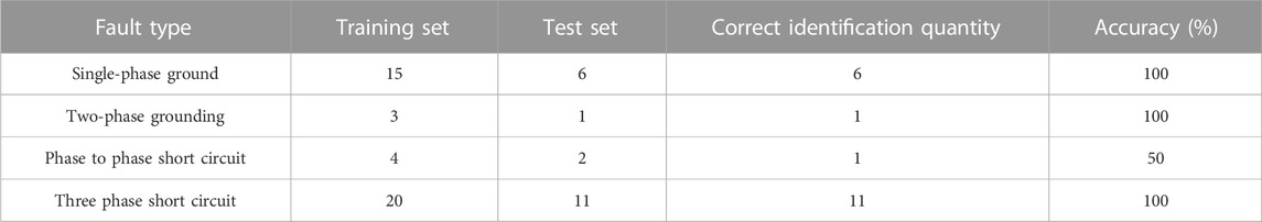
TABLE 5. Accuracy under different fault types.

From Table 5, it can be seen that the method proposed in this paper can accurately locate single-phase to ground, two-phase to ground, and three-phase short circuits at 100% accuracy. This is because at the simulation level, the probability of different faults occurring is considered, and the data for different faults is expanded. By freezing some layer parameters of the hidden layer (including weights, biases, and regularization coefficients), the migrated classification model includes both the characteristics of simulation samples and the laws of measured samples, To some extent, it compensates for the shortage of small samples in measured data and improves the accuracy of localization. For phase to phase short circuits, there are few measured samples and it is not possible to fully learn the sample patterns, resulting in a data localization error. Positioning to the adjacent line 19 can also reduce the inspection range to a certain extent.

Most existing studies use waveform data of voltage and current sampling values, which is difficult to obtain in practical engineering. Therefore, this article selects literature (Feng et al., 2023) that also uses sag amplitude data for comparative analysis of methods. However, literature (Feng et al., 2023) requires voltage sag values from all nodes to determine the location of sag sources through RBF neural networks. However, in practice, only a few nodes are installed with monitoring terminals due to the cost factor of monitoring terminals, resulting in the inability to obtain all node sag value data in actual examples. Therefore, this article selects the simulation data from Table 3 of the original text (including all node amplitudes) for comparative verification. The data distribution for the training and testing sets is shown in Table 6, and the results of temporary source localization are shown in Table 7.

TABLE 6

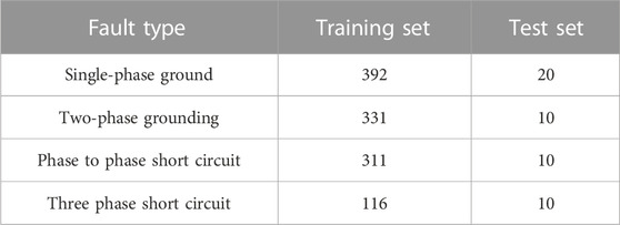
TABLE 6. Partition of simulation data training and testing sets.

TABLE 7

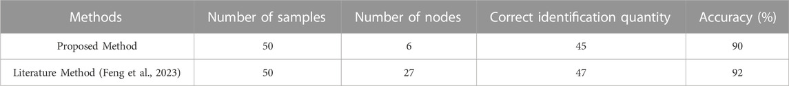
TABLE 7. The positioning results of the method in this article and literature (Feng et al., 2023)

As listed in Table 7, the accuracy of the proposed method is similar to the accuracy of the literature (Feng et al., 2023). However, the literature (Feng et al., 2023) requires the sag amplitude data of all nodes. Considering the actual data, the method in this paper only needs the sag amplitude data at the nodes with monitoring terminals, which greatly reduces the dependence on logarithmic data and the difficulty of engineering implementation.

Meanwhile, since voltage sag occurrences result from the joint action of faults and power grid structure, this method also takes into account fault type information and power grid structure situation, making the proposed algorithm more reasonable regarding data source acquisition and data selection. In addition, the methods presented in this paper also consider that the simulation data have the characteristics of large quantity and easy access, and also have a certain similarity with the measurement data. In contrast, the measurement data is small, and the data distribution is uneven. The simulation data is employed for pre-training, while the measurement data is modified to achieve transfer learning. Thus, the final model reflects both the characteristics of the simulation samples and the laws of the measurement samples, which makes up for the lack of small samples of the measurement data to some extent, thereby improving the accuracy of locating the temporary source section.

6 Conclusion

In this paper, based on the amplitude data of the sag event list of the monitoring system, combined with the advantages of easy access to simulation data and a large amount of data, a voltage sag source localization method is proposed, relying on multi-layer perceptron and Transfer learning. The efficacy of the proposed method has been verified by data from a certain region in East China, and the following conclusions have been drawn.

1) The data required in this paper only includes the amplitude of monitoring node sag, without the need for sampling waveform data. This characteristic reduces the cost of data transmission, storage, and calculation. The data can be obtained from the existing system employed by the power supply company, which has engineering practicality.

2) The proposed method fully considers the characteristics of simulation and measured data and uses Transfer learning to realize the complementary advantages offered by the two data types. The results of numerical examples indicate that the method’s accuracy in this paper is as high as 95% using simulation and measured data for positioning. Moreover, the number of iterations decreases by 27.8% compared to using only measured data. In addition, the positioning accuracy and convergence rate of the model are improved compared to other training methods.

3) Although this paper exploits the advantages of simulation data to a certain extent, it is still limited by common attributes. Therefore, future research focuses on expanding the combination space between simulation and measurement data and optimizing the final positioning model. In addition, the proposed method may fail when the same type of fault occurs at the end of the line and the first section of the next line under the same power grid architecture. Improving the reliability of the algorithm is an important direction for future research.

Data availability statement

The raw data supporting the conclusions of this article will be made available by the authors, without undue reservation.

Author contributions

RJ is the corresponding author and takes primary responsibility. TL contributed for the analysis of the work and wrote the first draft of the manuscript. All authors contributed to the article and approved the submitted version.

Funding

This work was supported by China Southern Power Grid Technology Project (Item No: 073000KK52200018).

Conflict of interest

Authors TL, ZW, and, YL were employed by Hainan Power Grid Co., Ltd.

The remaining author declares that the research was conducted in the absence of any commercial or financial relationships that could be construed as a potential conflict of interest.

Publisher’s note

All claims expressed in this article are solely those of the authors and do not necessarily represent those of their affiliated organizations, or those of the publisher, the editors and the reviewers. Any product that may be evaluated in this article, or claim that may be made by its manufacturer, is not guaranteed or endorsed by the publisher.

Supplementary material

The Supplementary Material for this article can be found online at: https://www.frontiersin.org/articles/10.3389/fenrg.2023.1237239/full#supplementary-material

References

Chen, R. S., Lin, T., Bi, R. Y., Xu, X. L., and Qi, Q. (2019). Strategy to precisely locate voltage sag source in active distribution grid with data measurement by limited power quality observations. Trans. China Electrotech. Soc. 34 (S1), 312–320. doi:10.19595/j.cnki.1000-6753.tces.180695

CrossRef Full Text | Google Scholar

Deng, Y., Liu, X., Jia, R., Huang, Q., Xiao, G., and Wang, P. (2021). Sag source location and type recognition via attention-based independently recurrent neural network. J. Mod. Power Syst. Clean Energy 9 (5), 1018–1031. doi:10.35833/MPCE.2020.000528

CrossRef Full Text | Google Scholar

Feng, Z. Y., Li, J. W., Zheng, C., Li, Q. L., and Jiang, J. D. (2023). Locating method of voltage sag source based on digital mirroring technology. Eng. J. Wuhan Univ. 56 (01), 36–43. doi:10.14188/j.1671-8844.2023-01-005

CrossRef Full Text | Google Scholar

Hamdan, I., Ibrahim, Ahmed M. A., and Noureldeen, O. (2020). Modified STATCOM control strategy for fault ride-through capability enhancement of grid-connected PV/wind hybrid power system during voltage sag. SN Appl. Sci. 2 (3), 364–419. doi:10.1007/s42452-020-2169-6

CrossRef Full Text | Google Scholar

Hopson, J. B., Neji, R., Dunn, J. T., McGinnity, C. J., Flaus, A., Reader, A. J., et al. (2023). Pre-training, transfer learning and pretext learning for a convolutional neural network applied to automated assessment of clinical PET image quality. IEEE Trans. Radiat. Plasma Med. Sci. 7 (4), 372–381. doi:10.1109/TRPMS.2022.3231702

PubMed Abstract | CrossRef Full Text | Google Scholar

Hu, A. P., Jiang, Y. J., Tao, Y. B., Sun, H. T., and Yi, H. (2021). Voltage sag source location in distribution networks based on wavelet energy entropy. Adv. Technol. Electr. Eng. Energy 40 (05), 50–56. doi:10.12067/ATEEE2101004

CrossRef Full Text | Google Scholar

Hu, W. X., and Xiao, X. Y. (2020). Influence of grid structure on voltage sag propagation and its quantitative analysis method. Electr. Power Autom. Equip. 40 (07), 1881–1894. doi:10.16081/j.epae.202006009

CrossRef Full Text | Google Scholar

Huang, J.X., Lin, Z., and Liu, K,Z. (2022). Association rule mining analysis method considering massive events in converter stations. Power Syst. Prot. Control, 50 (12), 117–125. doi:10.19783/j.cnki.pspc.211148

CrossRef Full Text | Google Scholar

Jia, R., Zhang, Y., Lin, H. W., and Chen, J. T. (2023). Homology identification of multi voltage sag events based on perceptual hash sequence. Power Syst. Prot. Control 51 (03), 133–144. doi:10.19783/j.cnki.pspc.220702

CrossRef Full Text | Google Scholar

Liu, Y., Xiao, X. Y., Zhang, X. P., and Wang, Y. (2020). Multi-Objective optimal STATCOM allocation for voltage sag mitigation. IEEE Trans. Power Deliv. 35 (03), 1410–1422. doi:10.1109/TPWRD.2019.2947715

CrossRef Full Text | Google Scholar

Lu, W. Q. (2020). Research on fault source location and severity evaluation method of voltage sag. North China Electric Power University. Beijing, China.

Google Scholar

Lv, G., Chu, C., Zang, Y., and Chen, G. (2021). Voltage sag source location estimation based on optimized configuration of monitoring points. CPSS Trans. Power Electron. Appl. 6 (3), 242–250. doi:10.24295/CPSSTPEA.2021.00023

CrossRef Full Text | Google Scholar

Lv, G. Y., Jiang, X. W., Hao, S. P., Lin, F., Cheng, H. Z., Zhang, X. Y., et al. (2019). Location of voltage sag source based on semi-supervised SVM. Power Syst. Prot. Control 47 (18), 76–81. doi:10.19783/j.cnki.pspc.181222

CrossRef Full Text | Google Scholar

Meng, Q. W., Gao, H., Zhong, Z. F., and He, J. Y. (2022). Voltage sag source location method based on Comparison of upstream positive sequence parameters. Automation Electr. Power Syst. 46 (13), 177–186. doi:10.7500/AEPS20211013003

CrossRef Full Text | Google Scholar

Mohammadi, Y., Moradi, M. H., and Chouhy, L. R. (2017). Locating the source of voltage sags: Full review, introduction of generalized methods and numerical simulations. Renew. Sus-tainable Energy Rev. 77 (9), 821–844. doi:10.1016/j.rser.2017.04.017

CrossRef Full Text | Google Scholar

Parsons, A. C., Grady, W. M., Powers, E. J., and Soward, J. (2000). A direction finder for power quality disturbances based upon disturbance power and energy. IEEE Trans. Power Deliv. 15 (3), 1081–1086. doi:10.1109/61.871378

CrossRef Full Text | Google Scholar

Si, X. Z., Li, Q. L., and Yang, J. L. (2017). Analysis of voltage sag characteristics based on measurement data. Electr. Power Autom. Equip. 37 (12), 144–149. doi:10.16081/j.issn.1006-6047.2017.12.020

CrossRef Full Text | Google Scholar

Tang, Y., Wei, R. M., Li, P., Qi, W. Z., and Li, G. (2014). Prognostic significance of KAI1/CD82 in human melanoma and its role in cell migration and invasion through the regulation of ING4. Automation Electr. Power Syst. 41 (06), 86–95. doi:10.1093/carcin/bgt346

CrossRef Full Text | Google Scholar

Wang, J. X., Zhang, Y., Chen, J. T., Wei, W., Wang, S. F., Yu, L. Y., et al. (2021). Evaluation of provincial power grid voltage sag and optimal selection of potential power supply points for industrial users. Electr. Power Autom. Equip. 41 (08), 201–210. doi:10.13287/j.1001-9332.202101.012

CrossRef Full Text | Google Scholar

Yang, G. J., Wang, K., Gao, W., et al. (2022). High impedance fault detection in a distribution network based on phase space reconstruction and transfer learning. Power Syst. Prot. Control 50 (13), 151–162. doi:10.19783/j.cnki.pspc.211282

CrossRef Full Text | Google Scholar

Yang, Z., Ma, Y. C., Li, L., Li, X., and Ma, Z. Y. (2022). A novel method for voltage sag source location based on hht and GA-BP. Electr. Power 55 (03), 97–104. doi:10.11930/j.issn.1004-9649.202007250

CrossRef Full Text | Google Scholar

Zhang, J., Zhou, Y. X., Hu, H., and Bian, Y. W. (2021). Identification of usefulness for online reviews based on knowledge adoption model and multilayer perceptron neural network. Chin. J. Manag. Sci. 30 (04), 264–274. doi:10.16381/j.cnki.issn1003-207x.2020.2215

CrossRef Full Text | Google Scholar

Zhang, Y., Wu, Y. F., Li, C. D., and Chen, J. T. (2023). Voltage sag risk assessment based on fusion of simulated and measurement data. Automation Electr. Power Syst., 1–15. doi:10.7500/AEPS20220928008

CrossRef Full Text | Google Scholar