 Till Strunge
 Phil Renforth
 Mijndert Van der Spek
- 1Research Institute for Sustainability—Helmholtz Centre Potsdam (Formerly Institute for Advanced Sustainability Studies, IASS), Potsdam, Germany
- 2Research Centre for Carbon Solutions, School of Engineering and Physical Sciences, Heriot-Watt University, Edinburgh, United Kingdom
The pathways toward net-zero greenhouse gas emissions by 2050 should be designed based on solid scientific evidence. Ex ante system analysis tools, such as techno-economic assessments (TEAs), are key instruments to guide decision-makers. As ex ante TEAs of CO2 mitigation technologies embody a high level of uncertainty, the informed use of uncertainty analysis becomes crucial for meaningful interpretation and communication of TEA outputs. To foster enhanced appreciation and the use of uncertainty analysis, we compare multiple uncertainty analysis methods for ex ante TEAs, using a case study on CO2 mineralization in the cement industry. We show that local sensitivity analysis tools such as one-way analysis, which are most often used by TEA practitioners, may not suffice for deriving reliable conclusions and provide guidance on how to apply global sensitivity analysis methods, such as variance-based indicators for TEAs in this field.
1 Introduction
Data-driven decision-making on the research and development (R&D) and investment in CO2 mitigation technologies, such as carbon capture and utilization (CCU) technologies, is key to achieving the goal of reaching net-zero greenhouse gas emissions by 2050. However, i) many technologies and systems are still at a low level of maturity, ii) underlying physio-chemical mechanisms have often not yet been fully investigated, iii) the level of process or system design is still preliminary, and iv) future environmental conditions (financial, policy, technology development, societal, etc.) cannot yet be fully anticipated. All the approaches and technologies needed to meet our climate goals do not exist at the scale and/or maturity needed. Ex ante system analysis tools that embody a high level of uncertainty (Van der Spek et al., 2021; Mendoza et al., 2022), among which techno-economic assessments (TEAs) for the evaluation of economic performance and life-cycle assessments (LCAs) for the evaluation of environmental impacts are needed to guide decision-makers in this process (Cremonese et al., 2020; Strunge et al., 2022a; Langhorst et al., 2022).
The rigorous use of uncertainty analysis methods has been advocated to increase the transparency of techno-economic studies and improve their utility (Van der Spek et al., 2017a; Van der Spek et al., 2017b; Van der Spek et al., 2020; Rubin et al., 2021; Van der Spek et al., 2021). TEA studies take different forms thorough the development process of the technology, from simplified studies using mass and energy balances to very detailed ones based on high-fidelity technology modeling (and/or measured plant data) and bottom-up costing methods (i.e., by starting with the design and costing of each major equipment) (Van der Spek et al., 2020). In principle, the uncertainty analysis methods used must fit the complexity of the TEA model and its purpose. For instance, an effective design for tax relief programs for CO2 storage requires TEA models of incumbent technologies, which can appropriately incorporate potential tax reliefs (Fan et al., 2018). Additionally, some uncertainty analysis methods come with high computational costs and data requirements, whereas others are much more straightforward to undertake, both considerations requiring TEA modelers to rationally weigh which method(s) to select for a given case. This is not trivial, and most frequently, the simplest uncertainty analysis methods are selected (i.e., local sensitivity analysis methods). For example, a non-exhaustive review of 21 studies presenting TEAs of CO2 mineralization processes showed that 11 publications (50%) used simple local sensitivity analysis methods (either one-at-a-time sensitivity analysis (Pedraza et al., 2021) or one-way sensitivity analysis (Huijgen, 2007; Huijgen et al., 2007; Hitch and Dipple, 2012; Pasquier et al., 2016; Naraharisetti et al., 2019; McQueen et al., 2020), and ten publications (45%) did not include any uncertainty analysis (Kakizawa et al., 2001; Iizuka et al., 2004; Katsuyama et al., 2005; O’Connor, 2005; Gerdemann et al., 2007; Eloneva, 2010; Sanna et al., 2012; Pérez-Fortes et al., 2014; Sanna et al., 2014; Mehleri et al., 2015). Only one publication (5%) applied a global sensitivity analysis method (Strunge et al., 2022b). We must acknowledge that more recent studies appeared to be more likely to incorporate some form of uncertainty analysis, highlighting the evolvements of this research field in recent years. Seemingly, when uncertainty analysis is incorporated, methods other than local sensitivity analysis are usually neglected and/or methods are selected without a clear rationale, possibly leading to errors in their use and especially the interpretation of model outputs. A result may be that conclusions are drawn on, for instance, economic viability that is not supported by the performed local sensitivity analysis of the uncertain input data.
Here, we present a tutorial case study where we discuss and show the use of a range of quantitative uncertainty analysis methods to inform TEA practitioners on the different options available, their use and utility, and good and, perhaps, poor practices. Overall, we aim to advance the appreciation and use of uncertainty analysis in the ex ante TEA literature to strengthen the quality of the TEAs that are undertaken, leading to a better-informed policy.
As a case study for techno-economic modeling of CCU technologies, we used an integrated TEA model of a CO2 mineralization process that produces a supplementary cementitious material (SCM) as cement replacement, as reported earlier in Strunge et al. (2022b). We discuss in detail seven common approaches to uncertainty analysis that may be relevant to the TEA of CO2 mitigation technologies (i.e., one-at-a-time sensitivity analysis, one- and multiple-way sensitivity analysis, scatterplot analysis, rank correlation, variance-based methods, and density-based methods) while acknowledging that many other methods (for specific other applications) have been developed (e.g., classification tree analysis if an analysis of smaller subsets of the input and output space is necessary or entropy mutual information analysis for non-monotonic relationships (Mishra et al., 2009)).
2 Case study and modeling
2.1 CO2 mineralization for SCM production
Being a major emitter of anthropogenic CO2 (Favier et al., 2018) with one of the highest carbon intensities per unit of revenue (Czigler et al., 2020), the cement industry needs economically viable solutions to reduce emissions and reach net zero (European Cement Association, 2014; Bellmann and Zimmermann, 2019; Czigler et al., 2020). For this sector, among other strategies, CO2 mineralization has been proposed as a means of CO2 utilization, where CO2 is reacted with activated minerals (e.g., magnesium- or calcium-rich minerals such as forsterite (Mg2SiO4) present in olivine-bearing rocks or lizardite (Mg3Si2O5(OH)4) present in serpentine-bearing rocks). As an exemplification, the mineralization reaction of CO2 with forsterite is shown as follows:
The product [mixture of carbonate (i.e., in the case of forsterite (MgCO3) and silica (SiO2))] can be used as an SCM in the cement industry. SCMs are materials that can be added to cement blends to archive certain properties or, more commonly, lower the amount of clinker (the cement’s main reactive component) needed in cement blends to reduce emissions (Favier et al., 2018). The by-product of CO2 mineralization silica makes the product mixture a valuable SCM for cement blends. Amorphous silica is a widely accepted pozzolanic additive in cement production. While the main product, carbonate, is inert when added to cement, amorphous silica and calcium hydroxide (CaOH) present in cement react to produce additional binding products (e.g., calcium silicate hydrates), leading to a comparable or increased strength to using cement alone (Wong and Abdul Razak, 2005). Hence, mineralization products not only permanently store CO2 as carbonates but also reduce emissions by partially replacing conventional cement/clinker production when used as SCMs (Sanna et al., 2012; Sanna et al., 2013; Benhelal et al., 2018; Woodall et al., 2019; Ostovari et al., 2020; Ostovari et al., 2021).
In Strunge et al. (2022b), we showed via integrated techno-economic modeling that the application of CO2 mineralization for the production of SCM could generate a net profit of up to €202132 per tonne of cement under certain conditions (i.e., the resulting products must be used as SCMs in cement blends and the storage of CO2 in minerals must be eligible for emission certificates or similar).
The CO2 mineralization process considered here is a direct aqueous carbonation approach based on Eikeland et al. (2015) and Gerdemann et al. (2007) (Figure 1; Supplementary Figure S1), in which ground minerals are reacted with captured CO2 in a pressurized stirred tank using an aqueous slurry with additives. We advanced this process by designing a post-processing train that i) partially separates unreacted minerals via gravity separation and ii) separates magnesium carbonate (MgCO3) from the reaction products, able to produce SCMs with different properties [i.e., different silica (SiO2) contents] (Strunge et al., 2022b; Kremer et al., 2022). We selected the conditions with the lowest costs as the nominal case (i.e., olivine-bearing rocks were used as feed minerals, the reaction pressure was set at 100 bar, and the reaction temperature was set at 190°C) (Strunge et al., 2022b). For this case study, the mineralization plant was assumed to be located at the cement plant’s site (located in the north of Germany) to reduce the costly transport of flue gas or CO2. As feed minerals (i.e., olivine-bearing rocks) are currently mined in Norway, Italy, Greece, or Spain (Kremer et al., 2019), they are transported to the mineralization plant, where they are first mechanically activated via crushing and grinding (pre-treatment), followed by the mineralization in continuously stirred reactors under elevated pressure and temperature, in an aqueous slurry with carbonation additives (i.e., NaCl and NaHCO3). CO2 is introduced in gaseous form into the mineralization slurry after being separated from the flue gas via monoethanolamine (MEA) post-combustion capture. Following the reaction, the slurry and unreacted minerals are recycled, and the products are purified (post-treatment) to produce an SCM for the cement industry (Figure 1). This purification step is needed as the carbonation reaction produces magnesium carbonate and silica. Because the former is inert when blended with cement, thus reducing its compressive strength, and the latter reacts with cement (i.e., increasing its strength), the silica content has to be increased through purification to use the carbonation products as SCM (Bremen et al., 2022; Strunge et al., 2022b; Kremer et al., 2022). Consequently, some of the inert products must be landfilled (e.g., in the limestone quarry) (Figure 1).
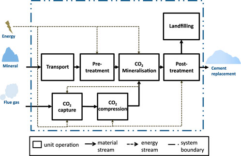
FIGURE 1. System boundaries of carbon capture utilization via mineralization model, adapted from Strunge (2021). Process flowsheet shown in Supplementary Figure S1.
The integrated TEA model, as is commonly the case, combines multiple approaches. We calculated mass and energy balances from first principles (e.g., energy transfer for heat exchangers) in combination with literature values (e.g., energy demand for grinding). The reaction conditions (e.g., pressure, temperature, and concentration) and resulting yield were based on literature values. A post-processing train did not exist yet and was therefore designed and subsequently simulated on Aspen Plus (Strunge et al., 2022b).
2.2 TEA model implementation
We described the methodology of the used TEA model in depth earlier in Strunge et al. (2022b). Hence, the following gives only a short overview of the approach followed. The model was developed following recent guidelines for TEA in CCU (IEAGHG, 2021; Rubin et al., 2021; Langhorst et al., 2022). The performance indicator chosen for this assessment was the levelized cost of product (LCOP) in €2021 per tonne SCMCCU produced. This indicator combines the total capital requirements (TCR) and operational expenditures (OpEx). We discounted the capital costs using the interest rate
We calculated the TCR building up from the total direct cost (TDC) and total overnight cost (TOC) (Eqs 4, 5, 6):
Here,
N characterizes the number of plants built, LR the learning rate, E the experience factor, i the interest during construction, and
We estimated OpEx using mass and energy balances as a basis to calculate the costs of utilities and feedstocks and the costs of material transport:
where the amount of feedstock or utility needed is represented by
The model was specified in MATLAB 2019b, which allowed for combining the technical and economic performance estimation into one model and running local and global sensitivity analysis methods on the integrated TEA model. For all global uncertainty analysis calculations, we used UQLab v1.4.0 (Marelli and Sudret, 2014), which is fully MATLAB-based, to easily link it to the TEA model.
2.3 Quantity of interest and selected input variables for the uncertainty analyses
For the case study, we used the output variable LCOP as the so-called quantity of interest (a term often used in uncertainty quantification for the output parameter of which the sensitivity is tested) to compare the different uncertainty analysis methods. We chose to vary the following input variables (Table 1).
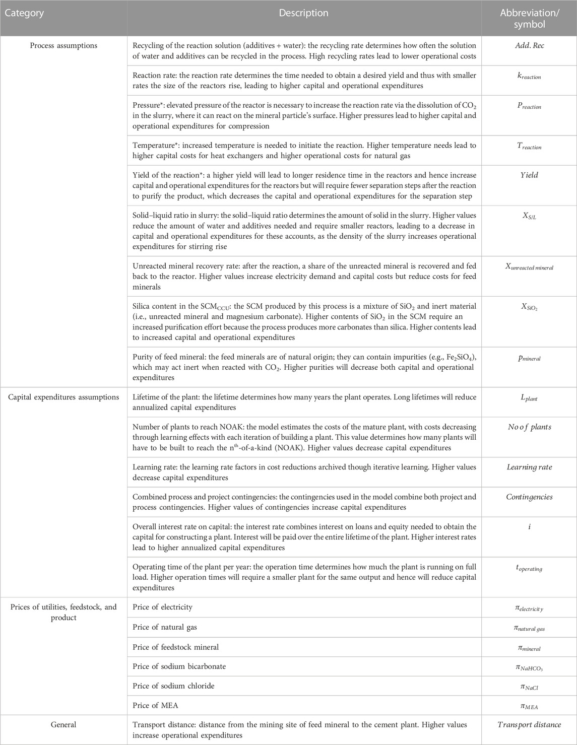
TABLE 1. Used input variables for the uncertainty analyses. *Only used in local sensitivity analysis because these variables are dependent on each other (e.g., yield of the reaction increases with pressure not modeled in the TEA model).
3 Uncertainty analysis methods in TEA
This section discusses the uncertainty analysis method we investigated here. It first gives a general introduction to uncertain TEA problems before discussing local sensitivity analysis in more detail. It then introduces global sensitivity analysis methods and approaches to characterize uncertainty and variability in model inputs.
A general formulation of an uncertain TEA problem can be specified as a function
As many parameters or variables of the input space
A helpful categorization of uncertainty was suggested by Rubin (2012), who distinguishes between “uncertainty,” “variability,” and “bias.” Although true uncertainty means the precise value of a parameter is not yet known (e.g., reaction yield of the process at scale), variability simply means a variable can take on different values (e.g., over a time period or at different locations) and the modeler chooses one (e.g., the temperature in a certain location). The principal difference between uncertainty and variability is that the precise value of uncertain parameters is not known, nor is the probability of the parameter taking on a certain value, whereas variable parameters are known or at least knowable, allowing quantification of a probability density function. This does not mean an uncertain parameter should not be quantified, they can and need to be, but their quantification is a guess or good estimate at best, rather than a (series of) measured value(s) per se. The uncertainty analysis methods discussed in this study can be used to assess uncertainty and variability, and hereafter, we refer to both simply as uncertainty. Bias refers to assumptions that (intended or unintended) change the results (e.g., choosing the highest or lowest reported reaction yield for the assessment of a chemical process) (Rubin, 2012; Van der Spek et al., 2020). Bias analysis is challenging as only third-party reviews of a study’s assumptions, and their reasoning might be able to detect these (Rubin, 2012).
The goals of uncertainty analyses can be manifold, including testing the robustness of a model and providing insight into changes in outputs due to changes in inputs and their probabilities to determine key drivers of uncertainty and gain insights into the strength of the model or its input data (Saltelli et al., 2008; Van der Spek et al., 2020). In this study, we focused on the commonly used goal to determine key drivers of uncertainty on the output of the model (i.e., creating a ranking of the most influential parameters on the model’s uncertainty) and investigated their input–output relationships, frequently called sensitivity analysis (Mishra and Datta-Gupta, 2018). In the following, we give an overview of seven suggested sensitivity analysis methods (Table 2).
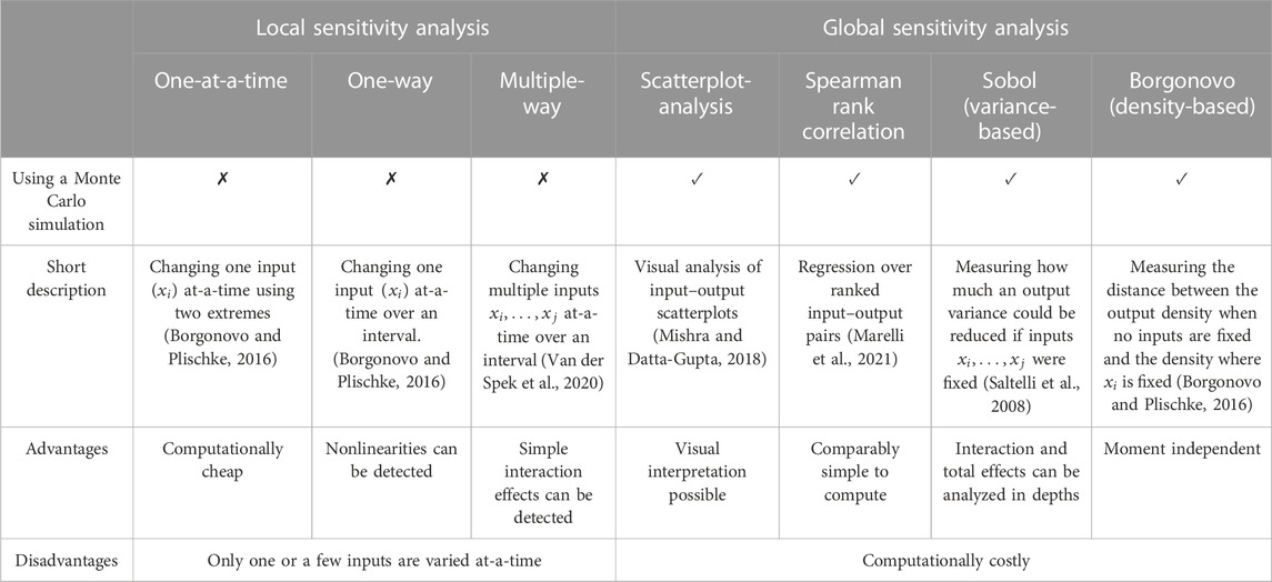
TABLE 2. Uncertainty analysis methods considered in this publication.
3.1 Local sensitivity analyses
Local sensitivity analyses (LSA) are the most commonly used methods in ex ante TEA, in which one or multiple input variables are varied around a base value. The simplest form of local analysis is the one-at-a-time (OAT) local sensitivity analysis, in which input variables of interest
We can then plot the output responses for each varied input
Another commonly used approach is one-way local sensitivity analysis, which is an extension of the OAT approach. Instead of using only two realizations of each input variable around the base value, a modeler varies the input variables using predefined intervals (e.g., ten steps in the predefined interval of
A drawback of these two methods is that no interaction effects can be investigated, as in each run, only one variable is changed at a time (Borgonovo and Plischke, 2016; Van der Spek et al., 2020; Van der Spek et al., 2021). However, most TEA models are likely to contain interaction effects because they often contain related parts. For example, process variables that impact capital expenditures might have a different influence on the LCOP depending on the interest on capital. To tackle this in a simple way, multiple-way sensitivity analysis can be used (Borgonovo and Plischke, 2016). Like the one-way local sensitivity analysis, input variables vary along a predefined interval, but instead of only varying one input variable, multiple variables are changed at a time. For example, variable pairs are varied in a two-way approach, and variable triplets are varied in a three-way approach. This allows modelers to identify combinations of variables with a high impact on the output that might not have been discovered using one-way analysis. The computational costs are significantly higher compared to the other local sensitivity analysis measures. This analysis requires
3.2 Global sensitivity analyses
Although local sensitivity analyses require comparably low computational costs, a major drawback is their limited ability to consider probabilities; hence, some considered realizations (e.g.,
3.3 Uncertainty characterization
The uncertainty characterization of the input parameters is arguably the most important step in probabilistic uncertainty/sensitivity analysis and requires experience and careful balancing of real knowledge of the uncertainty versus the ambitions of the modeler (e.g., a modeler might be drawn to choosing overly optimistic or pessimistic values to fit their goal). Often, we are inclined to fit probability density functions to collected data without accounting for its quality (e.g., completeness), leading to the propagation of incorrect or incomplete uncertainty, directly impacting the PDF of the parameter of interest. Care should be taken, for instance, to maintain PDFs within a range that is physically possible. For example, many quantities have natural limits (e.g., you cannot have a negative number of people). Multiple methods have been suggested to assist the modeler in selecting their uncertainty characterization (Harr, 1984; Hawer et al., 2018; Mishra and Datta-Gupta, 2018; Van der Spek et al., 2020; Van der Spek et al., 2021). We here exemplify three approaches that can help TEA practitioners define reasonable PDFs: i) a decision tree by Hawer et al. (2018), ii) the maximum entropy principle (Harr, 1984), and iii) simply choosing a uniform distribution for all inputs.
i) Hawer et al. (2018) (in the following referred to as Hawer’s method) provided a useful decision tree that gives suggestions on the probability density functions that should ideally be assigned, mainly depending on the data quality and nature (e.g., discrete or continuous) of the input parameter (Supplementary Figure S2). The decision tree guides the modeler to assign PDFs either subjectively by relying on assumptions on a potential distribution (e.g., through assessing the likelihood to have outliers in the dataset) or when more data are available, more objectively (e.g., through estimating a PDF using a maximum likelihood method on a dataset). This uncertainty characterization method can result in many different PDFs being assigned to the input variables (e.g., uniform, triangular, normal, logistic, and lognormal). Although we find this a comprehensive method for assigning PDFs, many options require detailed knowledge of the data, which may not always be publicly available for new or commercially sensitive technologies.
ii) An approach that requires slightly less knowledge is the maximum entropy principle, where five different types of PDF are assigned (uniform, triangular, normal, beta, and Poisson) (Harr, 1984), subject to known constraints in the available data (e.g., the bounds and mean, Supplementary Table S1). The general idea of this approach is to use all available information but not to add assumptions to estimate the PDFs (Mishra and Datta-Gupta, 2018). In comparison to Hawer’s method, the maximum entropy principle uses fewer options for describing the input data.
iii) The simplest method of assigning probability densities is assigning a uniform distribution in which all realizations have the same probability. This approach requires the least knowledge of the input parameters and can be performed by only knowing or defining a range for each input variable.
Although all approaches to assigning a PDF aim to harmonize under which conditions a certain PDF is assigned, modelers’ choices and interpretation of the underlying data quality inherently introduce a bias, which needs careful consideration. A method to reduce this bias can be the definition of several subjective probability distributions by multiple experts (Mishra and Datta-Gupta, 2018). Here, the modeler relies on multiple experts to, for example, estimate quantiles of distribution (e.g., minimum value relates to the 0th quantile and maximum value relates to the 100th quantile). Although this method can reduce the modeler’s bias, many TEA practitioners might not have access to experts for performing these estimations. Therefore, this approach is not discussed further in this article. In any case, TEA practitioners and the users of TEA results should always consider that even well-quantified PDFs only represent reality but may not capture it completely.
3.4 Uncertainty importance evaluation
Several approaches have been developed to describe the uncertainty importance of the output space
3.4.1 Scatterplot analysis
Scatterplots are suited to illustrate bivariate relationships and allow a visual determination of input–output relationships. Therefore, we plot the output sample of output j (
The computational costs for scatterplot analyses are significantly higher than those for local methods (Mishra and Datta-Gupta, 2018). Although the number of runs will depend on the nature of the model itself, most models will require at least C = 100–1,000 runs to reach convergence (Saltelli et al., 2008; Mishra and Datta-Gupta, 2018).
3.4.2 Spearman rank correlation
The Spearman rank correlation coefficient (SRCC) assesses how well the relationship between the input sample
The underlying assumption for using this measure is that the input–output relationship is characterized by a monotonic function (i.e., no inflection must be present in the relationship) (Helton et al., 1991), which first needs to be established, for instance, by visual inspection of the input–output relation. As the SRCC can be seen as the linear regression between the ranks, a non-monotonic function will not lead to sufficient answers (as the ranks are not linear) (Marelli et al., 2021), or it might not be possible to assign ranks at all if a value appears twice.
The computational costs for this method again depend on the nature of the model and require at least C = 100–1,000 runs (Saltelli et al., 2008; Mishra and Datta-Gupta, 2018).
3.4.3 Sobol indices
Variance-based methods assess how the expected variance of the output model changes when knowing an input realization with certainty. In the variance-based method, the indices by Sobol (1993) are commonly used (Borgonovo and Plischke, 2016). These variance based indices allow modelers not only to provide a quantitative measurement of the strength, direction, and nature of the global input–output relationship as the first sensitivity (i.e., the effect of one input variable alone on the output space), but also to investigate higher orders of input–output relationships (i.e., the effect of multiple variables collectively on the output space). Usually, the first-order effect and the total order effect are calculated and compared, which can uncover the interaction effects of input variables (which cannot be identified using the other suggested methods) (Borgonovo and Plischke, 2016). As Sobol’s variance-based measure depends on a particular moment of the output distribution (its variance), it may lead to misleading results when input variables influence the entire output distribution without significantly influencing the variance (Borgonovo and Tarantola, 2008).
The general idea for calculating Sobol indices lies in the decomposition of the model function (Eq. 11), in which
Following Sobol (1993), we define the total and partial variance for inputs
The first-order and higher-order indices
Because the calculation of each partial variance can be cumbersome and quickly makes thousands or millions of calculations be computed, multiple shortcut methods have been proposed (Saltelli et al., 2008; Marelli et al., 2021). For this study, we used the Janon estimator (Janon et al., 2014) (Eq. 16), allowing quick calculation of first-order and total-order effects. We considered two independent Monte Carlo samples
The computational costs for Sobol indices are significantly higher than other global sensitivity methods. Using the Janon estimator to calculate first-order and total-order indices, the required model runs are
3.4.4 Borgonovo indices
Because Sobol indices are moment dependent (i.e., the second moment: variance), Sobol indices cannot sufficiently analyze the sensitivities of inputs if they cannot be fully measured by the variance, which can, for example, be the case if selected PDFs for inputs have long tails (Borgonovo, 2007). Density-based approaches have been developed to counter this, which take the shape of the output distributions and compare it to the shape of the input distributions. Borgonovo (2007) developed the density-based method we used in this study.
We calculated the Borgonovo indices using the conditional and unconditional probability distribution function
To compute these, we used the histogram-based approach, which is used by default in UQLab (Marelli and Sudret, 2014; Marelli et al., 2021). To approximate the conditional distribution
The computational costs of this measure are again dependent on the nature of the model but can be expected to be at least C = 100–1,000 runs.
4 Results and illustration of uncertainty analysis methods
This section discusses the implementation of the deliberated uncertainty analysis methods in the mineralization case study. We first calculated the results using the base case assumptions (Table 3) for a mineralization plant with a capacity of 272 ktSCM a−1 (this size was chosen to replace 20% of cement of a cement plant producing 1.36 Mtcement a−1), leading to a levelized cost of the product of €129 tSCM−1 produced via CO2 mineralization. As previously discussed by Strunge et al. (2022b), these costs can be offset by replacing cement production and reducing the costs for CO2 emission certificates (e.g., from the European Emission Trading System). In the following, we applied the in Section 3 discussed uncertainty analysis tools (i.e., one-at-a-time sensitivity analysis, one- and multiple-way sensitivity analysis, scatterplot analysis, rank correlation, Sobol analysis and Borgonovo analysis ) to the case study.
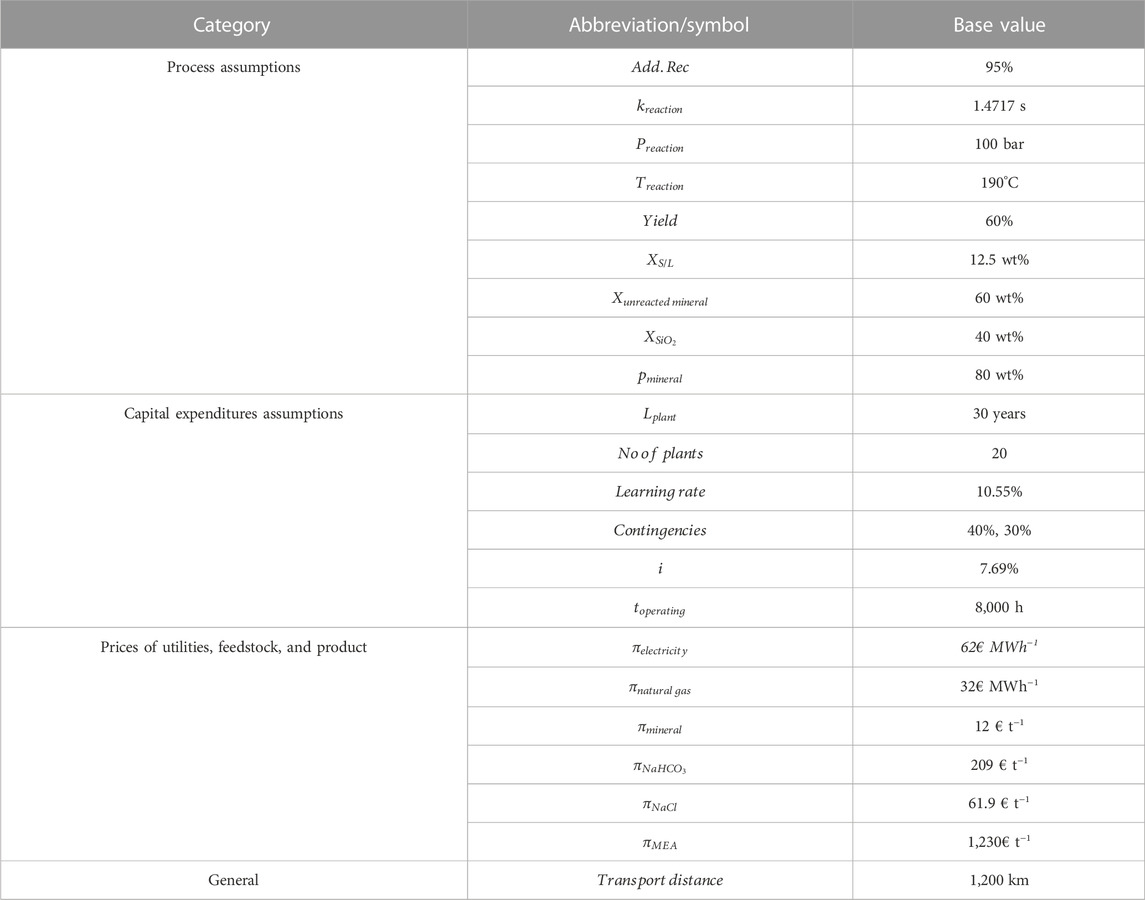
TABLE 3. Base case assumptions.
4.1 Exemplification of local sensitivity analysis methods
For the OAT sensitivity analysis, we varied the input variables around the base values by
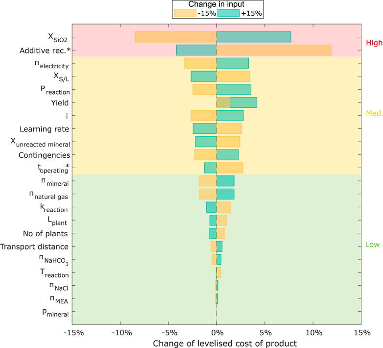
FIGURE 2. Results from OAT. Input variables are varied
For the one-way local sensitivity analysis, we varied the input values in 10 steps (including the extremes) within the interval of
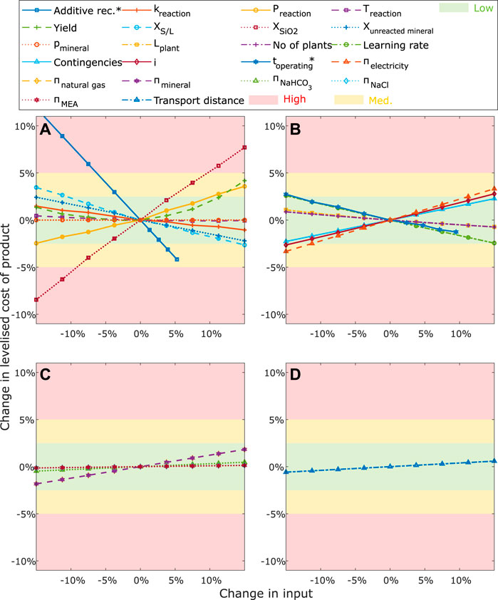
FIGURE 3. Results from one-way LSA. Input variables are varied
We performed the two-way sensitivity analysis on the six inputs with the highest impacts (Figure 4). This analysis aimed to investigate which combination of these inputs has a particularly high impact on the output and thus need to be investigated thoroughly. To interpret the results, we again clustered the local sensitivities following the induced change in the output (
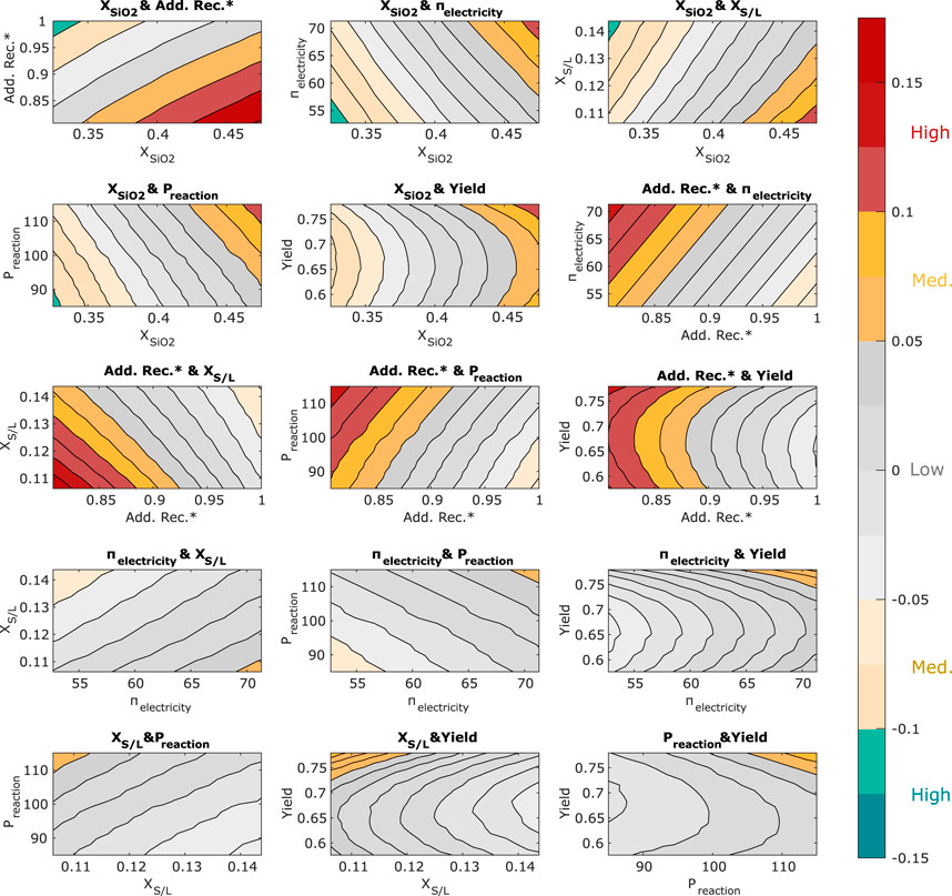
FIGURE 4. Results from two-way LSA. The six most influential input variables determined via OAT are varied in combination
The results show that nine combinations, including the variables
4.2 Exemplification of uncertainty characterization methods
Following the exemplification of LSA methods, we applied the aforementioned global sensitivity analysis methods to the case study. For the comparison of global uncertainty analysis methods, we removed dependent inputs (i.e.,
This section illustrates how uncertainty characterization (i.e., the selection of PDFs) can influence the output of a Monte Carlo simulation by applying the three methods discussed in Section 3.3 (i.e., Hawer’s method, maximum entropy principle, and assigning uniform distributions) to our case study. With different PDF choices resulting from the three methods, the uncertainty quantification moreover depends on the confidence of the modeler to determine certain moments of the distribution (e.g., mean and variance). In the approaches by Hawer et al. (2018) (i.e., Hawer’s method) and the maximum entropy approach of Harr (1984), a modeler with low confidence (pessimistic) in the data quality will choose simple distributions (e.g., a triangular distribution), whereas modelers with higher confidence (optimistic) in the data quality will be inclined to assign more complex methods (e.g., selecting a normal distribution or beta distribution). To exemplify this effect, we applied the maximum entropy principle, assuming high and low confidence in the data. The derived input samples and the selected PDFs are shown in Figure 5 and Supplementary Table S2.
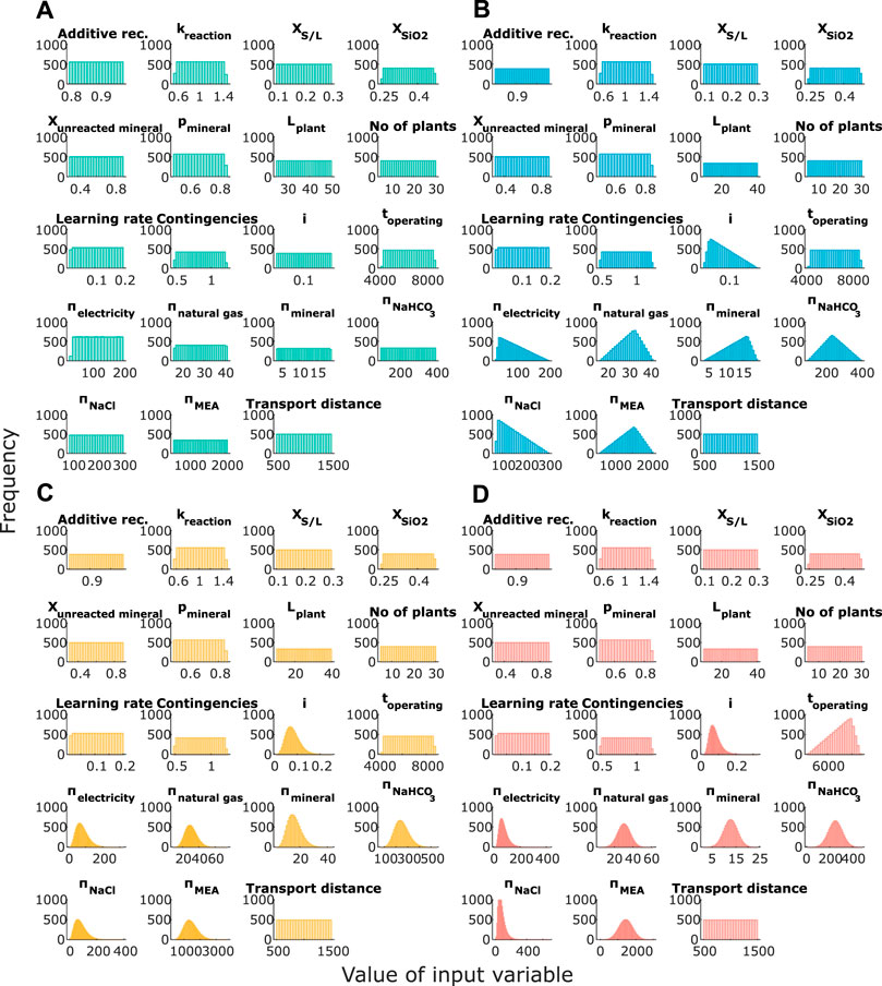
FIGURE 5. Input samples following different uncertainty characterization approaches: (A) uniform, (B) maximum entropy (pessimistic), (C) maximum entropy (optimistic), and (D) Hawer’s decision tree. Altering the input variables, additive recovery (
Figure 5 shows that for these inputs with the highest uncertainty (where a probability density is truly unknown, mostly process-related inputs in this case study, e.g.,
A comparison of the resulting output distributions when using the different uncertainty quantification methods reveals clear differences in the shape of the distribution and the mean and the width of the confidence interval for the quantity of interest (here, levelized cost of product) (Figure 6). First, note that the mean values, so the expected value from the MCSs (altering all variables at the same time), derived here (€145–€173 tSCM−1; see Figure 6), are in a similar range or exceed the maximum values for LCOP obtained using LSA methods (maximum value from OAT €144 tSCM−1, from two-way analysis €156 tSCM−1; see Section 4.1), which some might consider as extremes in the LSA. The use of uniform input distributions for all variables results in the highest mean (20% higher than using Hawer’s method) and (naturally) leads to an increase of approximately 25% in the width of the 95% confidence interval compared to applying Hawer’s method. A difference can additionally be seen between the maximum entropy principle (optimistic) and Hawer’s method. The results suggest that higher values of the output are less likely to follow Hawer’s method than when following the maximum entropy principle. This might be because we fit beta distributions to variables with high data availability following the maximum entropy principle assuming a confident modeler, whereas we fit lognormal and normal distributions when applying Hawer’s method. Although this effect will not always be statistically significant, given the unknown nature of some of the input parameters, which method has the highest accuracy cannot generally be concluded. However, we can conclude that different uncertainty quantification methods generate different output distributions. Therefore, particular care shall be taken when using MCS outputs for decision-making: someone cannot claim to provide a 95% confidence interval of an output if the exact nature of the input PDF is unknown, although this is very commonly done. Furthermore, clear communication of the assigned PDFs (and rationale) for MCSs must be a key element of ex ante system analyses to increase transparency and informed interpretation of results.
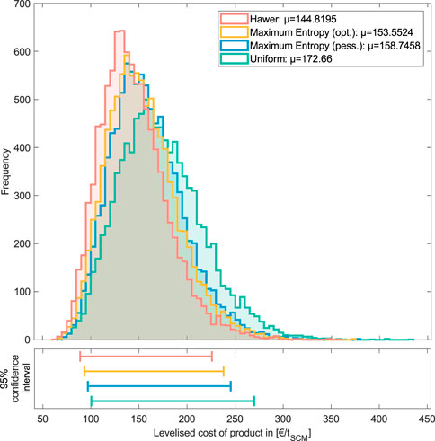
FIGURE 6. Comparison of the LCOP output distributions using different uncertainty characterization methods showing the frequency, mean (
4.3 Exemplification of uncertainty importance evaluation methods
We applied the aforementioned methods for measuring uncertainty importance (Section 3.4) to the case study. We here used Hawer’s method for uncertainty characterization. Note that for the comparison of the uncertainty importance evaluation methods, we again cluster the variables subjectively into three categories (high sensitivity, medium sensitivity, and low-to-no sensitivity). In contrast to the used categories for the LSA methods in Section 4.1, here, the values of the indices do not translate into a practical interpretation (e.g., an increase in LCOP by 10%).
In the scatterplot analysis, the visual determination of the most influential input variables concluded that
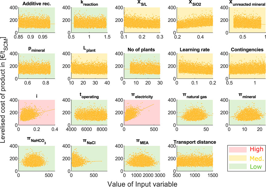
FIGURE 7. Results of scatterplot analysis. Variables with high sensitivity marked in red, medium sensitivity marked in yellow, and low sensitivity marked in green. Altering the input variables, additive recovery (
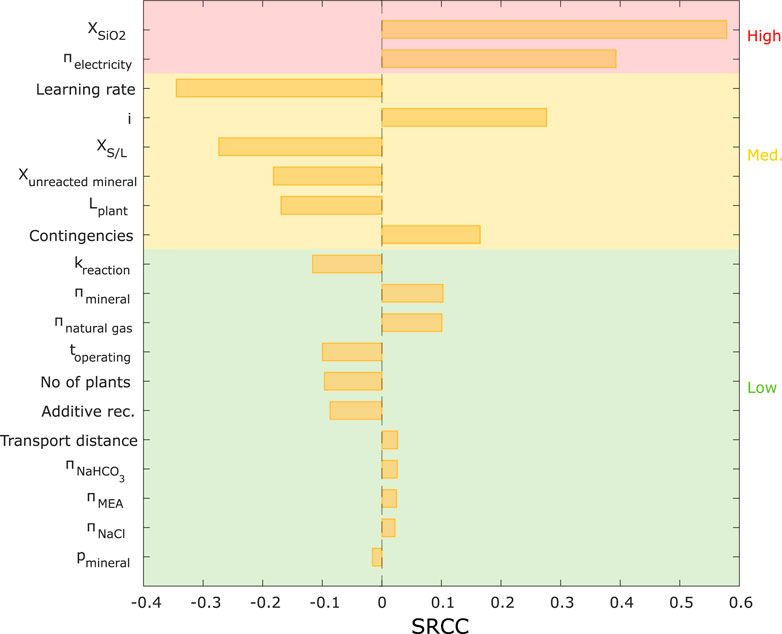
FIGURE 8. Results of SRCC analysis.
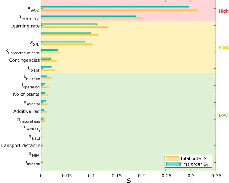
FIGURE 9. Results of Sobol analysis.
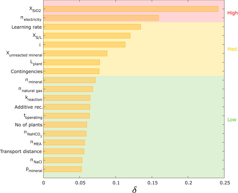
FIGURE 10. Results of Borgonovo analysis.
5 Discussion
The rankings of all input variables on the output described in Sections 4.1, 4.3 are summarized in Figure 11, where they are compared to the Sobol index (which, as the most comprehensive method, is often considered the gold standard among sensitivity indicators) (Roussanaly et al., 2021).
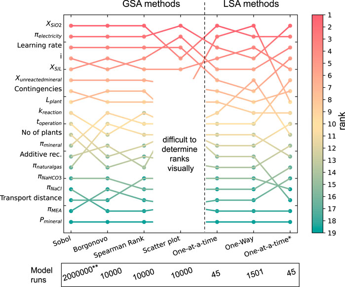
FIGURE 11. Comparison of ranks derived from each sensitivity analysis method. Variables only used in the LSA but not in the GSA are not shown. *For the second OAT, the same boundaries were used as for the GSA methods. **Model convergence for the Sobol indices was only found at
Figure 11 shows that the scatterplot method could only be used for a limited number of rankings because determining minor differences in the plots was challenging. All other global SA methods led to an almost unanimous ranking with only a few switches in positions (in particular for the first eight ranks), whereas there are noticeable differences with the rankings provided by the local SA methods (Figure 11). Using LSA methods, the uncertainty importance of some variables was highly overestimated (e.g.,
To compare the derived rankings quantitively, we applied the approach suggested by Ikonen (2016) to first transform rankings into Savage scores, followed by a correlation analysis to analyze the consistency between the uncertainty analysis methods. Savage scores were developed by Savage (1956) and had the advantage that inputs with higher ranks (i.e., 1st or 2nd) receive a significantly higher score, whereas less influential parameters receive very similar scores (Supplementary Equation S1). Calculated Pearson correlation coefficients (PCC) (Supplementary Equation S2) between the Savage scores of the uncertainty analysis methods are shown in Table 4. The results confirm that, in this case study, the GSA methods (i.e., SRCC, Sobol indices, and Borgonovo indices) showed high consistency in the results (a PCC close to the maximum value of 100% was reached, indicating an almost perfect correlation between the derived rankings). However, the correlation between LSA and GSA methods shows a much lower strength (PCC of 77%–87% for OAT and PCC of 54%–91% for one-way sensitivity analysis).
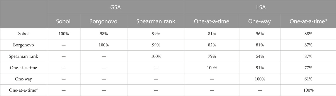
TABLE 4. Pearson correlation coefficients between the calculated Savage scores for the rankings of each uncertainty analysis method. Scatterplot analysis was excluded as it did not yield a ranking for each variable (Figure 11). *For the second OAT, the same boundaries were used as for the GSA methods.
Although the correlation between the GSA approaches was high, small changes in ranks were expected as they are all calculated differently and have slightly different underlying assumptions. The results of the GSA methods show that position switches mainly occurred to variables with underlying interaction effects (i.e., in this case study:
6 Summary and recommendations
The case study and analyses in this publication lead to a number of general recommendations on the use of uncertainty analysis in ex ante TEA studies. We showed that LSA methods can be insufficient in identifying all inputs of high importance and characterize inputs as important while they may not be. Therefore, we recommend the wider use of global SA methods to improve the utility of uncertainty analysis in ex ante TEAs and make such studies more valuable for policy- and decision-making.
This study also showed the effect of using different uncertainty characterization approaches for GSA, where the characterization method used and the confidence of the modeler can have a non-negligible influence on the computed confidence intervals, thus communicating the message. Therefore, policy- and decision-making should only rely on computed confidence intervals when there is high confidence in the inputted probability density functions (indicating they represent variability rather than true uncertainty) and when all known information has been used by the modeler. Given that this is seldomly true for ex ante studies, we argue against using GSA to answer strictly prognostic (what will) type of questions in the ex ante technology/system analysis domain but limit the use of GSA to identify sensitivities instead.
Regarding uncertainty importance evaluations, all quantitative GSA methods used in this case study (i.e., SRCC, Sobol, and Borgonovo) could compute consistent ranking orders (i.e., the results were largely the same). Because Sobol analysis entails much higher computational costs, it may suffice to use SRCC or Borgonovo indices instead. However, we first recommend investigating the presence and severity of interaction effects (e.g., through only using a smaller group of variables for the Sobol analysis or through multiple-ways LSA) because interaction effects are likely to cause changes in rankings between the used methods. SRCC or Borgonovo indices should then preferably be applied when small or no interaction effects are present. In particular, this may be of major importance with more complex and/or nonlinear models.
In conclusion, we recommend ex ante TEA modelers to i) use LSA methods only when computational power is truly limited, ii) refrain from using GSA of ex ante techno-economic models for answering prognostic questions, iii) investigate parameter interactions a priori and use Sobol indices when significant interaction effects are present or can be expected, and iv) otherwise use SRCC or Borgonovo (or other “cheap”) indices to avoid high computational costs. The results from this study suggest that using these recommendations will not only harmonize the results from different TEA studies but also increase their utility for public and private policy- and decision-making.
Data availability statement
The datasets presented in this study can be found in online repositories. The names of the repository/repositories and accession number(s) can be found at: https://doi.org/10.5281/zenodo.7863667.
Author contributions
TS: conceptualization, methodology, formal analysis, and writing—original draft. PR: conceptualization and writing—review. MV: conceptualization, methodology, formal analysis, and writing—review. All authors contributed to the article and approved the submitted version.
Funding
TS has been funded by the global CO2 initiative as part of the project CO2nsistent and received a scholarship at Heriot-Watt University. PR and MV are funded through the UK’s Industrial Decarbonization Research and Innovation Centre (EP/V027050/1).
Conflict of interest
The authors declare that the research was conducted in the absence of any commercial or financial relationships that could be construed as a potential conflict of interest.
Publisher’s note
All claims expressed in this article are solely those of the authors and do not necessarily represent those of their affiliated organizations or those of the publisher, the editors, and the reviewers. Any product that may be evaluated in this article, or claim that may be made by its manufacturer, is not guaranteed or endorsed by the publisher.
Supplementary material
The Supplementary Material for this article can be found online at: https://www.frontiersin.org/articles/10.3389/fenrg.2023.1182969/full#supplementary-material
References
Anantharaman, R., Berstad, D., Cinti, G., De Lena, E., Gatti, M., Hoppe, H., et al. (2018). CEMCAP Framework for Comparative Techno-economic Analysis of CO2 Capture From Cement Plants-D3, 2. Zenodo.
Bellmann, E., and Zimmermann, P. (2019). Climate protection in the concrete and cement industry - background and possible courses of action. Berlin.
Benhelal, E., Rashid, M., Holt, C., Rayson, M., Brent, G., Hook, J., et al. (2018). The utilisation of feed and byproducts of mineral carbonation processes as pozzolanic cement replacements. J. Clean. Prod. 186, 499–513. doi:10.1016/j.jclepro.2018.03.076
Borgonovo, E. (2007). A new uncertainty importance measure. Reliab. Eng. Syst. Saf. 92 (6), 771–784. doi:10.1016/j.ress.2006.04.015
Borgonovo, E., and Plischke, E. (2016). Sensitivity analysis: A review of recent advances. Eur. J. Operational Res. 248 (3), 869–887. doi:10.1016/j.ejor.2015.06.032
Borgonovo, E., and Tarantola, S. (2008). Moment independent and variance-based sensitivity analysis with correlations: An application to the stability of a chemical reactor. Int. J. Chem. Kinet. 40 (11), 687–698. doi:10.1002/kin.20368
Bremen, A. M., Strunge, T., Ostovari, H., Spütz, H., Mhamdi, A., Renforth, P., et al. (2022). Direct olivine carbonation: Optimal process design for a low-emission and cost-efficient cement production. Industrial Eng. Chem. Res. 61, 13177–13190. doi:10.1021/acs.iecr.2c00984
Cremonese, L., Olfe-Kräutlein, B., Strunge, T., Naims, H., Zimmermann, A., Langhorst, T., et al. (2020). Making Sense of Techno-Economic Assessment & Life Cycle Assessment Studies for CO2 Utilization: A guide on how to commission, understand, and derive decisions from TEA and LCA studies. Ann Arbor: Global CO2 Initiative.
Czigler, T., Reiter, S., Schulze, P., and Somers, K. (2020). Laying the foundation for zero-carbon cement. Frankfurt: McKinsey & Company.
Eikeland, E., Blichfeld, A. B., Tyrsted, C., Jensen, A., and Iversen, B. B. (2015). Optimized carbonation of magnesium silicate mineral for CO2 storage. ACS Appl. Mater. interfaces 7 (9), 5258–5264. doi:10.1021/am508432w
Eloneva, S. (2010). Reduction of CO2 emissions by mineral carbonation: Steelmaking slags as rawmaterial with a pure calcium carbonate end product.
Fan, J.-L., Xu, M., Wei, S.-J., Zhong, P., Zhang, X., Yang, Y., et al. (2018). Evaluating the effect of a subsidy policy on carbon capture and storage (CCS) investment decision-making in China — a perspective based on the 45Q tax credit. Energy Procedia 154, 22–28. doi:10.1016/j.egypro.2018.11.005
Favier, A., De Wolf, C., Scrivener, K., and Habert, G. (2018). A sustainable future for the European Cement and Concrete Industry: Technology assessment for full decarbonisation of the. industry by 2050". ETH Zurich).
Gerdemann, S. J., O'Connor, W. K., Dahlin, D. C., Penner, L. R., and Rush, H. (2007). Ex situ aqueous mineral carbonation. Environ. Sci. Technol. 41 (7), 2587–2593. doi:10.1021/es0619253
Harr, M. E. (1984). Reliability-based design in civil engineering 20. Department of Civil Engineering, School of Engineering, North Carolina State University.
Hastie, T., Tibshirani, R., Friedman, J. H., and Friedman, J. H. (2009). The elements of statistical learning: Data mining, inference, and prediction. Springer.
Hawer, S., Schönmann, A., and Reinhart, G. (2018). Guideline for the classification and modelling of uncertainty and fuzziness. Procedia CIRP 67, 52–57. doi:10.1016/j.procir.2017.12.175
Helton, J. C., Garner, J. W., McCurley, R. D., and Rudeen, D. K. (1991). Sensitivity analysis techniques and results for performance assessment at the Waste Isolation Pilot Plant. (United States).
Hitch, M., and Dipple, G. (2012). Economic feasibility and sensitivity analysis of integrating industrial-scale mineral carbonation into mining operations. Miner. Eng. 39, 268–275. doi:10.1016/j.mineng.2012.07.007
Huijgen, W. J., Comans, R. N., and Witkamp, G.-J. (2007). Cost evaluation of CO2 sequestration by aqueous mineral carbonation. Energy Convers. Manag. 48 (7), 1923–1935. doi:10.1016/j.enconman.2007.01.035
IEAGHG (2021). Towards improved guidelines for cost evaluation of carbon capture and storage 2021-TR05.
Iizuka, A., Fujii, M., Yamasaki, A., and Yanagisawa, Y. (2004). Development of a new CO2 sequestration process utilizing the carbonation of waste cement. Industrial Eng. Chem. Res. 43 (24), 7880–7887. doi:10.1021/ie0496176
Ikonen, T. (2016). Comparison of global sensitivity analysis methods – application to fuel behavior modeling. Nucl. Eng. Des. 297, 72–80. doi:10.1016/j.nucengdes.2015.11.025
Janon, A., Klein, T., Lagnoux, A., Nodet, M., and Prieur, C. (2014). Asymptotic normality and efficiency of two Sobol index estimators. ESAIM Probab. Statistics 18, 342–364. doi:10.1051/ps/2013040
Kakizawa, M., Yamasaki, A., and Yanagisawa, Y. (2001). A new CO2 disposal process via artificial weathering of calcium silicate accelerated by acetic acid. Energy 26 (4), 341–354. doi:10.1016/S0360-5442(01)00005-6
Katsuyama, Y., Yamasaki, A., Iizuka, A., Fujii, M., Kumagai, K., and Yanagisawa, Y. (2005). Development of a process for producing high-purity calcium carbonate (CaCO3) from waste cement using pressurized CO2. Environ. Prog. 24 (2), 162–170. doi:10.1002/ep.10080
Kremer, D., Etzold, S., Boldt, J., Blaum, P., Hahn, K. M., Wotruba, H., et al. (2019). Geological mapping and characterization of possible primary input materials for the mineral sequestration of carbon dioxide in europe. Minerals 9 (8), 485. doi:10.3390/min9080485
Kremer, D., Strunge, T., Skocek, J., Schabel, S., Kostka, M., Hopmann, C., et al. (2022). Separation of reaction products from ex-situ mineral carbonation and utilization as a substitute in cement, paper, and rubber applications. J. CO2 Util. 62, 102067. doi:10.1016/j.jcou.2022.102067
Langhorst, T., McCord, S., Zimmermann, A., Müller, L., Cremonese, L., Strunge, T., et al. (2022). Techno-economic assessment & life cycle assessment guidelines for CO2 Utilization. Version 2.0. Ann Arbor: Global CO2 Inititativer.
Marelli, S., Lamas, C., Konakli, K., Mylonas, C., Wiederkehr, P., and Sudret, B. (2021). UQLab user manual – sensitivity analysis, Report # UQLab-V1.4-106. Switzerland: Chair of Risk, Safety and Uncertainty Quantification, ETH Zurich.
Marelli, S., and Sudret, B. (2014). “UQLab: A framework for uncertainty quantification in matlab,” in The 2nd international Conference on Vulnerability and risk Analysis and management (ICVRAM 2014)), 2554–2563.
McQueen, N., Kelemen, P., Dipple, G., Renforth, P., and Wilcox, J. (2020). Ambient weathering of magnesium oxide for CO2 removal from air. Nat. Commun. 11 (1), 3299. doi:10.1038/s41467-020-16510-3
Mehleri, E. D., Bhave, A., Shah, N., Fennell, P., and Mac Dowell, N. (2015). “Techno-economic assessment and environmental impacts of Mineral Carbonation of industrial wastes and other uses of carbon dioxide,” in Fifth international conference on accelerated carbonation for environmental and material engineering (ACEME 2015) (New York.
Mendoza, N., Mathai, T., Boren, B., Roberts, J., Niffenegger, J., Sick, V., et al. (2022). Adapting the technology performance level integrated assessment framework to low-TRL technologies within the carbon capture, utilization, and storage industry, Part I. Front. Clim. 4. doi:10.3389/fclim.2022.818786
Mishra, S., and Datta-Gupta, A. (2018). “Uncertainty quantification,” in Applied statistical modeling and data analytics, 119–167.
Mishra, S., Deeds, N., and Ruskauff, G. (2009). Global sensitivity analysis techniques for probabilistic ground water modeling. Groundwater 47 (5), 727–744. doi:10.1111/j.1745-6584.2009.00604.x
Naraharisetti, P. K., Yeo, T. Y., and Bu, J. (2019). New classification of CO2 mineralization processes and economic evaluation. Renew. Sustain. Energy Rev. 99, 220–233. doi:10.1016/j.rser.2018.10.008
O’Connor, W. K., Rush, G. E., Gerdemann, S. J., and Penner, L. R. (2005). Aqueous mineral carbonation: Mineral availability, pretreatment, reaction parametrics, and process studies. Albany: National Energy Technology Laboratory.
Ostovari, H., Müller, L., Skocek, J., and Bardow, A. (2021). From unavoidable CO2 source to CO2 sink? A cement industry based on CO2 mineralization. Environ. Sci. Technol. 55 (8), 5212–5223. doi:10.1021/acs.est.0c07599
Ostovari, H., Sternberg, A., and Bardow, A. (2020). Rock ‘n’ use of CO2: Carbon footprint of carbon capture and utilization by mineralization. Sustain. Energy & Fuels 4, 4482–4496. doi:10.1039/D0SE00190B
Pasquier, L.-C., Mercier, G., Blais, J.-F., Cecchi, E., and Kentish, S. (2016). Technical & economic evaluation of a mineral carbonation process using southern Québec mining wastes for CO2 sequestration of raw flue gas with by-product recovery. Int. J. Greenh. Gas Control 50, 147–157. doi:10.1016/j.ijggc.2016.04.030
Pedraza, J., Zimmermann, A., Tobon, J., Schomäcker, R., and Rojas, N. (2021). On the road to net zero-emission cement: Integrated assessment of mineral carbonation of cement kiln dust. Lausanne, Switzerland: Chemical engineering journal, 408. doi:10.1016/j.cej.2020.127346
Pérez-Fortes, M., Bocin-Dumitriu, A., and Tzimas, E. (2014). Techno-economic assessment of carbon utilisation potential in Europe. Chem. Eng. Trans.
Peters, M. S., Timmerhaus, K. D., and West, R. E. (1991). Plant design and economics for chemical engineers. International edition.
Roussanaly, S., Rubin, E. S., van der Spek, M., Booras, G., Berghout, N., Fout, T., et al. (2021). Towards improved guidelines for cost evaluation of carbon capture and storage. doi:10.5281/ZENODO.4643649
Rubin, E. S., Berghout, N., Booras, G., Fout, T., Garcia, M., Nazir, M. S., et al. (2021). “Chapter 1: Towards improved cost guidelines for advanced low-carbon technologies,” in Towards improved guidelines for cost evaluation of carbon capture and storage. Editors S. Roussanaly, E. S. Rubin, and M Van der Spek.
Rubin, E. S., Short, C., Booras, G., Davison, J., Ekstrom, C., Matuszewski, M., et al. (2013). A proposed methodology for CO2 capture and storage cost estimates. Int. J. Greenh. Gas Control 17, 488–503. doi:10.1016/j.ijggc.2013.06.004
Rubin, E. S. (2012). Understanding the pitfalls of CCS cost estimates. Int. J. Greenh. Gas Control 10, 181–190. doi:10.1016/j.ijggc.2012.06.004
Sagrado, I. C., and Herranz, L. E. (2013). "Impact of steady state uncertainties on ria modeling calculations", in LWR fuel performance meeting. Downers Grove: Top Fuel, 497–504.
Saltelli, A., Ratto, M., Andres, T., Campolongo, F., Cariboni, J., Gatelli, D., et al. (2008). Global sensitivity analysis. The Primer. John Wiley & Sons.
Sanna, A., Dri, M., and Maroto-Valer, M. (2013). Carbon dioxide capture and storage by pH swing aqueous mineralisation using a mixture of ammonium salts and antigorite source. Fuel 114, 153–161. doi:10.1016/j.fuel.2012.08.014
Sanna, A., Hall, M. R., and Maroto-Valer, M. (2012). Post-processing pathways in carbon capture and storage by mineral carbonation (CCSM) towards the introduction of carbon neutral materials. Energy & Environ. Sci. 5 (7), 7781. doi:10.1039/c2ee03455g
Sanna, A., Uibu, M., Caramanna, G., Kuusik, R., and Maroto-Valer, M. M. (2014). A review of mineral carbonation technologies to sequester CO2. Chem. Soc. Rev. 43 (23), 8049–8080. doi:10.1039/c4cs00035h
Savage, I. R. (1956). Contributions to the theory of rank order statistics-the two-sample case. Ann. Math. Statistics 27 (3), 590–615. doi:10.1214/aoms/1177728170
Sobol, I. (1993). Sensitivity estimates for nonlinear mathematical models. Math. Model. Comput. Exp. 1, 407–414.
Soepyan, F. B., Anderson-Cook, C. M., Morgan, J. C., Tong, C. H., Bhattacharyya, D., Omell, B. P., et al. (2018). “Sequential design of experiments to maximize learning from carbon capture pilot plant testing,” in Computer aided chemical engineering. Editors M. R. Eden, M. G. Ierapetritou, and G. P. Towler (Elsevier), 283–288.
Strunge, T., Naims, H., Ostovari, H., and Olfe-Kraeutlein, B. (2022a). Priorities for supporting emission reduction technologies in the cement sector – a multi-criteria decision analysis of CO2 mineralisation. J. Clean. Prod. 340, 130712. doi:10.1016/j.jclepro.2022.130712
Strunge, T., Renforth, P., and Van der Spek, M. (2022b). Towards a business case for CO2 mineralisation in the cement industry. Commun. Earth Environ. 3 (1), 59. doi:10.1038/s43247-022-00390-0
Strunge, T. (2022). Techno-Economic Model for "Towards a business case for CO2 mineralisation in the cement industry". doi:10.5281/zenodo.5971924
Strunge, T. (2021). “The cost of CO2 carbonation in the cement industry,” in TCCS-11 - trondheim Conference on CO2 capture, Transport and storage: SINTEF).
Strunge, T. (2023). Uncertainty analysis model for "uncertainty quantification in the techno-economic analysis of emission reduction technologies: A tutorial case study on CO2 mineralisation". v1.0.0-alpha. doi:10.5281/zenodo.7863667
Van der Spek, M., Fernandez, E. S., Eldrup, N. H., Skagestad, R., Ramirez, A., and Faaij, A. (2017a). Unravelling uncertainty and variability in early stage techno-economic assessments of carbon capture technologies. Int. J. Greenh. Gas Control 56, 221–236. doi:10.1016/j.ijggc.2016.11.021
Van der Spek, M., Fout, T., Garcia, M., Kuncheekanna, V. N., Matuszewski, M., McCoy, S., et al. (2021). “Chapter 3: Towards improved guidelines for uncertainty anaylsis of carbon captuer and storage techno-economic studies,” in Towards improved guidelines for cost evaluation of carbon capture and storage. Editors S. Roussanaly, E. S. Rubin, and M Van der Spek.
Van der Spek, M., Fout, T., Garcia, M., Kuncheekanna, V. N., Matuszewski, M., McCoy, S., et al. (2020). Uncertainty analysis in the techno-economic assessment of CO2 capture and storage technologies. Critical review and guidelines for use. Int. J. Greenh. Gas Control 100, 103113. doi:10.1016/j.ijggc.2020.103113
Van der Spek, M., Ramirez, A., and Faaij, A. (2017b). Challenges and uncertainties of ex ante techno-economic analysis of low TRL CO2 capture technology: Lessons from a case study of an NGCC with exhaust gas recycle and electric swing adsorption. Appl. Energy 208, 920–934. doi:10.1016/j.apenergy.2017.09.058
Wong, H. S., and Abdul Razak, H. (2005). Efficiency of calcined kaolin and silica fume as cement replacement material for strength performance. Cem. Concr. Res. 35 (4), 696–702. doi:10.1016/j.cemconres.2004.05.051
Keywords: uncertainty analysis, techno-economic assessment, carbon capture and utilization or, storage, CO2 mineralization
Citation: Strunge T, Renforth P and Van der Spek M (2023) Uncertainty quantification in the techno-economic analysis of emission reduction technologies: a tutorial case study on CO2 mineralization. Front. Energy Res. 11:1182969. doi: 10.3389/fenrg.2023.1182969
Received: 09 March 2023; Accepted: 04 May 2023;
Published: 26 May 2023.
Edited by:
Antonio Coppola, Istituto di Scienze e Tecnologie per l’Energia e la Mobilità Sostenibili—Consiglio Nazionale delle Ricerche, ItalyReviewed by:
Muhammad Imran Rashid, University of Engineering and Technology, Lahore, PakistanLouis-César Pasquier, Université du Québec, Canada
Copyright © 2023 Strunge, Renforth and Van der Spek. This is an open-access article distributed under the terms of the Creative Commons Attribution License (CC BY). The use, distribution or reproduction in other forums is permitted, provided the original author(s) and the copyright owner(s) are credited and that the original publication in this journal is cited, in accordance with accepted academic practice. No use, distribution or reproduction is permitted which does not comply with these terms.
*Correspondence: Till Strunge, dGlsbC5zdHJ1bmdlQHJpZnMtcG90c2RhbS5kZQ==; Mijndert Van der Spek, bS52YW5fZGVyX3NwZWtAaHcuYWMudWs=