 Changsheng Li1*
 Haoran Ma
95% of researchers rate our articles as excellent or good
Learn more about the work of our research integrity team to safeguard the quality of each article we publish.
Find out more
ORIGINAL RESEARCH article
Front. Energy Res. , 14 June 2023
Sec. Smart Grids
Volume 11 - 2023 | https://doi.org/10.3389/fenrg.2023.1174301
Nonlinear parity-time-symmetric wireless power transfer (NPTS-WPT) is a novel wireless power transfer technology. NPTS-WPT systems exhibit the resonant frequency bifurcation phenomenon in the strong coupling region. However, working frequency selection mechanisms and control methods for use in the bifurcation region remain unclear. In this study, the description function method was used to model and analyze the dynamics of NPTS-WPT systems. The frequency stability, evolution and convergence characteristics of resonant frequency bifurcation were studied for varying distances between the receiver (Rx) and transmitter circuits varies. In addition, the loop detuning characteristics and the mechanism by which the amplification factor of the operational amplifier influences the system’s frequency-hopping behavior were determined. The detuning rate must be greater than the detuning tolerance to cause resonant frequency-hopping. Moreover, we propose a method to induce changes in the natural frequency of the Rx circuit by adding a detuning control circuit at the Rx, thereby allowing the resonant frequency to be selected and controlled. Finally, the conclusions from the theoretical analysis and the feasibility of the proposed frequency control methods were validated using an experimental system. The proposed resonant frequency control methods offer a viable method for directional frequency selection and artificial frequency control in NPTS-WPT systems operating in the strong coupling region.
As a novel wireless power transfer (WPT) technology, the nonlinear parity-time-symmetric (NPTS) WPT (NPTS-WPT) system was first reported in 2017 in Nature (Assawaworrarit et al., 2017). The study reported that the transfer efficiency between coils with diameters of 58 cm can be maintained at approximately 100% when the distance between the coils is 20–70 cm after a nonlinear gain saturation mechanism is introduced into the parity-time (PT)-symmetric circuit containing the two coupled coils.
Compared with the electromagnetic induction method and the traditional magnetic resonance method, the distinctive characteristic of an NPTS-WPT system is that without the use of additional control circuit modules or software algorithms and by relying solely on the principal characteristics of the circuit, the output frequency of the drive circuit at the transmitter (Tx) is adjusted automatically when the distance between the receiver (Rx) and Tx coils changes or other parameters fluctuate. The Tx and Rx loops thus remain in a resonant state at all times, thereby maintaining stable and highly efficient power transfer efficiency within the specified range and exhibiting strong robustness.
NPTS-WPT has received increased research interest in recent years. In 2018 Younes Ra’di, in cooperation with Fu Liu et al., used electric field coupling between metal plates instead of the magnetic field coupling coils used in a previous study (Assawaworrarit et al., 2017), thereby expanding the power transfer coupling mode at the Rx and Tx circuits (Ra’di et al., 2018). In 2019, Fu Liu further optimized and improved the circuit topology and the principle prototype (Liu F. et al., 2019), and used pulse oscillation instead of single harmonic oscillation. This approach can maintain a transfer efficiency of more than 90% over a wide load fluctuation range. Based on the principle of the Duffing resonator, Abdelatty proposed a position-insensitive WPT system containing nonlinear capacitors (Abdelatty et al., 2019). This system provides a constant transfer efficiency of approximately 80% when the axial distance between the Tx and Rx coils is 15 ± 10 cm, the coil diameter’s lateral misalignment is ±50%, and the angular misalignment is ±75°. Zhang from South China University of Technology performed an innovative exploration of the NPTS topology for use in fields such as single-line electric field coupling power transfer (Shu and Zhang, 2018), constant-efficiency wireless charging for unmanned aerial vehicles based on magnetic field coupling (Zhou et al., 2019), and electric-magnetic field dual coupling WPT (Liu and Zhang, 2018). Compared with the traditional design (Assawaworrarit et al., 2017), the principal difference is that a half-bridge inverter is used instead of an operational amplifier (OP amp) as the Tx circuit driver, and the current signal extracted from this Tx circuit is taken as the feedback signal and used to control the operation of the half-bridge inverter switching tube, thereby yielding a nonlinear saturation gain and improved overall power transfer efficiency. In 2020, a Massachusetts Institute of Technology (MIT) team achieved stable and highly efficient WPT by using a class-E amplifier with current-sensing feedback in the PT-symmetric circuit (Assawaworrarit and Fan, 2020a). In their improved circuit, the PT symmetry ensures a constant effective load impedance for the switch amplifier. The amplifier continues to operate efficiently, even if the transmission distance changes. In a previous study (Zhou et al., 2020), NPTS-WPT technology was employed to read the circuit design of passive wireless sensors. The read-out distance was approximately four times as long as that obtained when using conventional WPT methods while maintaining the same sensitivity. Another study (Ishida et al., 2021) presented the design of a low-frequency NPTS-WPT system operating at frequencies below 20 kHz. A high transmission power of 7.6 W was achieved when the Rx and Tx coils were wound on a Mn-Zn ferrite core, and the Tx circuit used a high voltage OP amp. First, they created a transmission system circuit model by using the symmetric and asymmetric parameters of the Rx and Tx circuits. This model was based on the mutual inductance coupling theory, which is used in this paper. Next, they analyzed the effects of these parameters on the power transmission characteristics (Dong et al., 2019a; Li et al., 2020) and proposed a novel current-type NPTS circuit topology (Dong et al., 2019b).
The NPTS-WPT system drives the coupling coils by using the self-excited oscillation of an OP amp working in the nonlinear saturation region. Compared with switching inverters that are commonly used in electromagnetic induction and conventional magnetic resonance methods, NPTS-WPT provides low energy conversion efficiency and limited transmission power and is thus not suitable for use in high-power wireless transfer applications that require high overall transmission efficiency, such as electric vehicle wireless charging. However, because of outstanding advantages such as strong robustness, long transmission distance, and simple circuit topology, NPTS-WPT has broad application prospects in the field of low-power wireless charging, where distance variations and parameter fluctuations occur, such as information cross-linking between ammunition and weapons systems and where the provision of an external wireless power supply for implantable medical diagnostic equipment. As novel concept, the related research is still in its infancy.
Several studies have verified that in the strong coupling region, NPTS-WPT systems exhibit resonant frequency bifurcation (Assawaworrarit et al., 2017; Liu and Zhang, 2018; Shu and Zhang, 2018; Dong et al., 2019a; Dong et al., 2019b; Zhou et al., 2019; Assawaworrarit and Fan, 2020a; Li et al., 2020; Zhang, 2020; Zhou et al., 2020; Ishida et al., 2021; Yatsugi et al., 2021), which is similar to traditional magnetic resonance frequency characteristics (Nguyen and Agbinya, 2015; Liu M. et al., 2019; Song et al., 2021). Different resonant frequency points have an important impact on the system’s transmission efficiency and transmission distance. Most scholars consider that the frequency bifurcation phenomenon is not conducive to the operation of the system. The main research direction has been to adjust the circuit parameters to eliminate this phenomenon (Truong, 2021). However, the real-world WPT systems are not in a completely symmetrical state (Li et al., 2020), and the transmission power and efficiency at the two bifurcation frequencies are different. Thus, the transmission performance of the system can be improved by controlling and selecting the working frequency. Furthermore, this method can be used for simultaneous wireless power and information transfer (SWPIT) systems where the high and low frequencies represent information ‘1′and ‘0′respectively.
Although studies on magnetic resonance, they have discovered and explained the occurrence of the frequency bifurcation phenomenon, they have not offered an in-depth discussion on the evolution of change in the frequency or propose a method for selection and control of the resonant frequency. Because the NPTS-WPT system has two resonant frequency branches in the strong coupling region, which resonant frequency branch will be selected during practical operation, and whether there are any technical means to enable the system to hop from one resonant frequency branch to the other. We have created a dynamic model for an NPTS-WPT system by using the description function method (DFM) and used the model to study the resonant frequency bifurcation and frequency-hopping mechanisms. On this basis, we 0discussed the methods for the selection and control of the resonant frequency in the strong coupling region. Finally, we experimentally verified the correctness of the conclusion derived from the theoretical analysis and the feasibility of the proposed technical methods.
The typical circuit principle of an NPTS-WPT system is illustrated in Figure 1A. Resistor R1 and the OP amp form a negative resistance, which is used to convert part of the direct current (DC) into an alternating current (AC) to feed the WPT system. RF and RG are, respectively, the feedback and gain resistances of the OP amp. Through the appropriate design of the values of RF and RG, the required voltage amplification factor in the linear region of the OP amp is achieved. R2 is the load resistance of the Tx circuit. L1 and L2 are, respectively, the inductances of the Tx and Rx coils, and M is the mutual inductance of the two coils. R01 and R02 represent the internal resistances of the Tx and Rx coils, respectively. C1 and C2 are the matching capacitors for the Tx and Rx loops, respectively, and are used to set the natural frequencies of the Tx and Rx loops. V1 and V2 are the voltages across the Tx and Rx coils, respectively, and I1 and I2 are the currents that flow through the Tx and Rx coils, respectively.
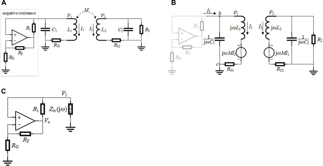
FIGURE 1. (A)Circuit diagram of an NPTS-WPT system. (B) Phasor model of the NPTS-WPT system. (C) Simplified circuit diagram of the NPTS-WPT system.
Refs (Assawaworrarit et al., 2017; Dong et al., 2019a) show that the steady-state voltage and current in this circuit are both sinusoidal signals; therefore, this circuit above can be simplified using the phasor method. The phasor model (without consideration of the negative resistance) is shown in Figure 1B.
According to Kirchhoff’s law,
The equivalent impedance between b and c can be obtained from Eq. 1 (while excluding the negative resistance) as follows:
where.
Therefore, the NPTS-WPT system can be simplified further, as illustrated in Figure 1C, where Vo is the output voltage of the OP amp.
The DFM is a common analytical method used for nonlinear systems, and can analyze aspects such as the stability and limit cycle of high-order nonlinear systems (Engelberg, 2002). The DFM is generally used to model power converters in power systems (Sinha et al., 2018). To use the DFM, the system must be analyzed in the s-domain. When the self-excited oscillation of the system and the independence of its characteristics from the initial state are considered, jω in Eq. 2 can be replaced with s, Accordingly, we obtain
When the functions of the OP amp are considered based on its virtual-short and virtual-break characteristics, Eqs. 4, 5 hold true:
The transfer function G(s) is defined using Eq. 4 as follows:
Additionally, the voltage amplification factor of an OP amp in the linear region, which is denoted as kOP, can be defined using Eq. 5 as follows:
The linear feedback block diagram of the system can be obtained using equations. (6) and (7), as shown in Figure 2A, where Vo is the input to G(s) and the output from kOP, and V1 is the output from G(s) and the input to kOP. This is similar to the aforementioned circuit diagram, where kOP is taken as the negative input to the OP amp. The block diagram of the nonlinear feedback considering the saturation nonlinearity of the OP amp shown in Figure 2B.

FIGURE 2. (A) Linear feedback block diagram of system. (B) Nonlinear feedback block diagram of the system.
Here, the description function for the saturation nonlinearity can be expressed as follows:
In Equation 8, where A is the signal amplitude [−a, a] represents the linear region of the OP amp, and a represents the saturation, which is illustrated in Figure 3A. The saturation of an OP amp depends on its supply voltage. For subsequent analysis, the saturations at various supply voltages were measured for the LM7171 OP amp, as shown in Figure 3B, where APS = (V+ − V−)/2, and V+ and V− are, respectively, the positive and negative supply voltages of the OP amp.
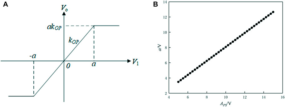
FIGURE 3. (A) Saturated nonlinear parametric diagram. (B) Relationship between a and supply voltage.
The characteristic equation of the nonlinear feedback system shown in Figure 2B is
Eq. 9 can be converted into the following:
where −1/N(A) is referred to as the negative reversal characteristic of the description function.
The transfer function for the linear portion of the system can be defined as follows:
where
The NPTS-WPT system has two resonant frequency points when operating in the strong coupling region. However, this system cannot simultaneously be operated at two frequency points—it must operate at one point or the other. This raises the questions of whether or not this choice is random and whether a system running at a specific frequency point can then hop to another frequency point for operation through artificial and technical means. These problems are in this section.
In this study, for an NPTS-WPT system with the parameters listed in Table 1, we determined the evolution process of the system’s resonant frequencies with changes in the distance between the Tx and Rx coils by using the DFM presented in Section II and then used the resonant frequency control method in the strong coupling region. The measured curve for the relationship between the coupling coefficient and the distance is shown in Figure 4. All calculational and experimental parameters used in this study are presented in Table 1 unless otherwise specified. The Rx and Tx coils are spiral coils with the same diameter of 90 mm. These coils were wound using enameled copper wires with a diameter of 1 mm. The number of turns for both coils is 7 and the power supply voltage is ±12 V.
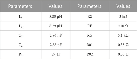
TABLE 1. Computational and experimental parameters.
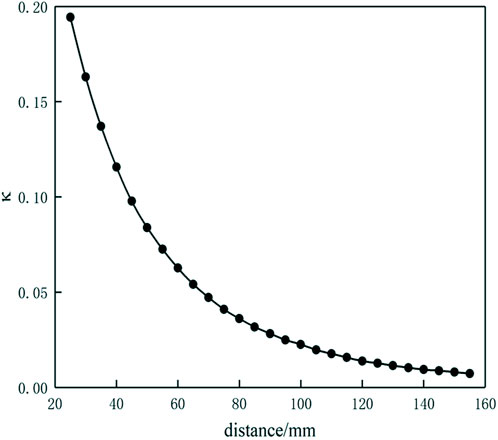
FIGURE 4. Curve of κ value versus distance between the coils.
The Nyquist diagram of H(s) and the image of −1/N(A) were drawn on the complex plane, with results as shown in Figure 5. The image of −1/N(A) on the complex plane was a ray on the negative real axis that started at (−1/kOP,0) and moved toward (−∞,0) with increasing A. The directions of the arrows shown in the figure were consistent with the growth direction of A. The Nyquist diagram of H(s) can only show the nonnegative angular frequency portion. The directions of the arrows on the curves indicate the direction in which ω is increasing. The value of ω at the intersection of H(s) and −1/N(A) is the solution to Eq. 11, i.e., the system resonance frequency. For example, in Figure 5B, the values of ω at the intersections are defined as ω1, ω2 and ω3, where ω3 ≥ ω2 ≥ ω1 > 0. These intersections can be either stable or unstable. Specifically, in the direction of the H(s) curve where it is increasing along ω, if the direction in which −1/N(A) is increasing with increasing A is from the right side of the H(s) curve toward the left side, then the intersection is stable; in contrast, if the direction in which −1/N(A) is increasing with increasing A is from the left side of the H(s) curve toward the right side, then the intersection is unstable.
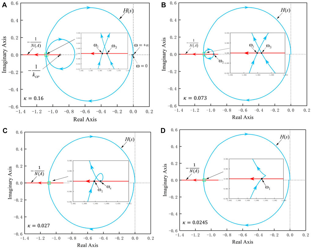
FIGURE 5. Images of H(s) and −1/N(A) on the complex plane: (A) κ = 0.16, (B) κ = 0.073 (C) κ = 0.27, and (D) κ = 0.0245. The stretched-out views are shown in the images at the intersections.
When the κ value was high (i.e., κ = 0.16, as shown in Figure 5A), H(s) and −1/N(A) intersected twice (corresponding to ω1 and ω3). According to the intersection stability judgment method described above, ω1 and ω3 were both stable and are thus represented by solid dots in the figure. In Figure 5B, κ = 0.073, and when compared with Figure 5A, the inner circle formed by H(s) is smaller because of the reduction in the value of κ. H(s) intersected with −1/N(A) thrice. ω1 and ω3 were stable in this case, while ω2 was unstable and was thus represented by a hollow dot in the figure. As κ decreased further, the inner circle formed by H(s) continued to shrink. When this shrinking circle was exactly tangential to the negative real axis, a critical state was reached, as illustrated in Figure 5C (where κ = 0.027). In addition, ω2 and ω3 converged into a point, represented by ωc in this case. Here, ωc represents the convergence of the original stable point ω3 and the unstable point ω2 is called the critical stable angular frequency and is represented by a half-solid dot in the figure. The corresponding coupling coefficient is denoted as κc and is called the critical coupling coefficient. When κ continued to decrease further, H(s) and −1/N(A) had only one intersection at ω1 and this frequency point was stable.
The resonant frequency curves for varying distances between the Tx and Rx coils are shown in Figure 6. The area in which κ > κc is called the strong coupling region. Here, the system had two stable, resonant frequency branches (i.e., f1 and f3), which are called the low-frequency branch and the high-frequency branch, respectively. In addition, there was an unstable intermediate frequency branch (i.e., f2) when the distance between the Tx and Rx coils was within a certain range of values. The intermediate frequency branch f2 cannot be observed experimentally because it is merely a theoretical solution derived from the theoretical analysis. As κ continued to decrease (and the distance between the Tx and Rx coils increased), the three resonant angular frequencies continued to approach each other and evolved into stable and critical stable, resonant angular frequencies at the critical distance. The area in which κ < κc is called the weak coupling region. In this case, the system exhibited only one stable resonant frequency branch. In the strong coupling region, when the distance between the two coils decreased, the difference between the high-frequency and low-frequency branches increased in tandem. However, in the weak coupling region, the resonant frequency of the system basically remained unchanged.
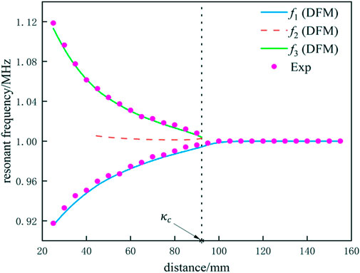
FIGURE 6. Curves of resonant frequency versus distance between coils.
Preliminary studies have found that artificial detuning between the Rx and Tx circuits can affect the system’s resonant frequency (Li and Huang, 2022; Liu et al., 2022; Wang et al., 2023). When the detuning rate is sufficiently high, the resonant frequency-hopping phenomenon occurs. For the WPT system shown in Figure 1A, changes in the inductance L2 or the resonance matching capacitance C2 will lead to a natural frequency offset at the Rx circuit. This may cause system detuning. Here, γ is defined as the natural frequency offset rate and can be expressed as follows:
where
Figure 7 shows the Nyquist curve for H(s) and the image of −1/N(A) at various values of γ. In the calculation example, γ was adjusted by changing the value of C2; κ = 0.073,
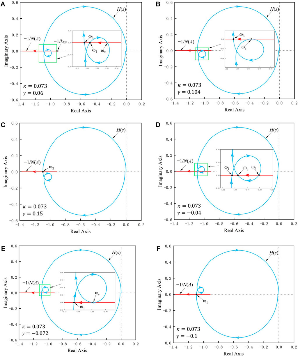
FIGURE 7. Graphics of H(s) and −1/N(A) on the complex plane during detuning when κ = 0.073: (A) γ = 0.06; (B) γ = 0.104; (C) γ = 0.15; (D) γ = - 0.04; (E) γ = - 0.072; (F) γ = - 0.1.
The case in which γ < 0 was analyzed next. The image where γ = −0.04 is shown in Figure 7D. Compared with Figure 5B, the inner circle formed by H(s) in this case shifted upward. According to the frequency stability analysis method, ω1 and ω3 were both stable resonant angular frequencies, while ω2 was again an unstable resonant angular frequency. When γ decreased continuously, ω3 and ω2 gradually approached each other and ultimately converged when γ = −0.072; this frequency point is also denoted by ωc, as shown in Figure 7E. When γ decreased further, there was only one intersection between H(s) and −1/N(A), as illustrated in Figure 7F. In this case, there was only the low-frequency branch ω1 in the system, and this frequency point was stable.
In summary, when γ > 0 and the value of γ increased continuously, the low frequency ω1 and the unstable point ω2 gradually moved closer to each other and ultimately converged into a critical stable frequency point before departing from the negative real axis. As a result, there was only the high-frequency resonance branch ω3 within the system. When γ < 0 and γ decreased continuously, the high frequency ω3 and the unstable point ω2 gradually moved closer to each other and ultimately converged into a critical stable frequency point before departing from the negative real axis. As a result, there was only the low-frequency resonance branch ω1 in the system.
Figure 8 shows the curves of variations in the resonant frequency with γ at various κ values. Using the curve plotted with κ = 0.073 as an example, on the high-frequency branch, when γ decreased continuously, the resonant frequency of the system climbed continually along the high-frequency branch; the resonant frequency then hopped from the high-frequency branch to the low-frequency branch when γ reached γ1. At this point, the system’s resonant frequency continued to move left along the low-frequency branch when γ was decreased further. On the low-frequency branch, when γ increased continuously, the system’s resonant frequency moved continually along the low-frequency branch; the resonant frequency then hopped from the low-frequency branch to the high-frequency branch when γ reached γ2. When γ continued to increase, then the resonant frequency of the system continued to move right along the high-frequency branch (Cao et al., 2022; Tang et al., 2022). Arrows mark the points γ1 and γ2 to indicate that this frequency-hopping behavior is uniaxial. This means that the resonant frequency of the system can only hop from the high-frequency branch to the low-frequency branch at point γ1, and the system cannot hop from the low-frequency branch to the high-frequency branch. Similarly, at point γ2, the resonant frequency of the system can only hop from the low-frequency branch to the high-frequency branch, and the system cannot hop from the high-frequency branch to the low-frequency branch.
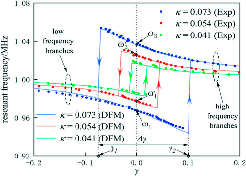
FIGURE 8. Frequency-hopping curves under incomplete symmetry condition.
However, the change in the resonant frequency is bidirectional and reversible before γ reaches either γ1 or γ2, regardless of whether the system runs on the high-frequency or low-frequency branch. In other words, if the system is operating on the high-frequency branch, the resonant frequency of the system will increase toward the left as γ decreases continuously. If γ then begins to increase before it reaches γ1, the resonant frequency of the system will return along the same route via the high-frequency branch and move downward to the right without hopping to the low-frequency branch (Assawaworrarit and Fan, 2020b; Hu et al., 2022; Hua et al., 2022). Similarly, if the system is running on the low-frequency branch, the resonant frequency will move down toward the right as γ increases continuously. If γ then begins to decrease before it reaches γ2, the resonant frequency of the system will return along the same route via the low-frequency branch and climb toward the left without hopping to the high-frequency branch.
The parameter Δγ (Δγ = γ2 − γ1) is defined as the detuning tolerance, which represents the maximum offset at which the system can maintain the original resonant frequency branch without hopping. As shown in Figure 8, the comparison of the three curves (for κ = 0.073, 0.054 and 0.041) shows that a larger value of κ corresponds to a larger Δγ. There was clearly only one resonant frequency within the system in this case, and the frequency-hopping behavior disappeared when the coupling coefficient was smaller than the critical coupling coefficient.
The variation and hopping mechanisms for the resonant frequency can be interpreted from the perspective of system stability. Parameter changes or external disturbances (e.g., changes in the equivalent values of the capacitance and inductance, κ values, and other parameters) that occur during system operation may cause changes in the resonant frequency. If there are still two stable resonant frequency points after the change to the new parameters, the system will opt to run at the stable point closest to the operating point identified before the parameter change, rather than at stable points far away from that operating point. “Close” and “far” here refer to the differences between the two resonant frequencies. The frequency points are clearly closer to each other when located on the same resonant frequency branch than when they are on different branches. However, if there is no longer a stable frequency point on the original operating frequency branch following the change in operating parameters, frequency-hopping becomes inevitable (Yang et al., 2022). Therefore, when the distance between the Tx and Rx coils gradually increases or decreases in the strong coupling region, the system operating frequency changes along the original resonant frequency branch, but not sharply. The operating frequency does not hop to another resonant frequency branch and thus causes an abrupt change unless the original frequency branch no longer exists. These resonant frequency selections and hopping processes make it clear that the system operation involves specific inertance and inertia properties.
According to the analysis presented above, the process of disappearance of a stable frequency branch involves three stages: stability, critical stability and disappearance. Critical stable points result from the convergence of the stable resonant frequency with the unstable resonant frequency, as illustrated in Figures 7B,E. However, in some cases, there may be no critical stable state, as in the example shown in Figure 9. Before their convergence, ω2 and ω3 no longer represent the roots of Eq. 12 or the intersections of H(s) and −1/N(A). The parameter difference between Figures 9, 7A is that the initial point of −1/N(A) shifted to the left in Figure 9 because the amplification factor kOP decreased from 1.1 to 1.01 within the linear region of the OP amp. In addition, the frequency-hopping event occurs prematurely because ω1, which was supposed to be a stable frequency point, becomes an unstable point. Clearly, kOP plays an important role in the frequency-hopping behavior.
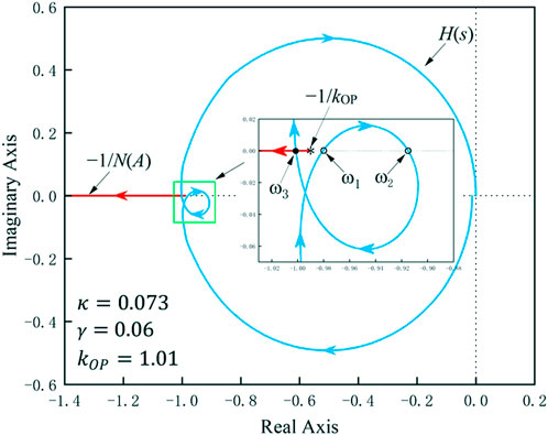
FIGURE 9. Hopping before frequency convergence.
Figure 10 shows the system frequency-hopping diagram for several different values of kOP, with the values of the rest of the parameters remaining unchanged. The value of kOP can be adjusted by varying the RG value. As the figure shows, the detuning tolerance Δγ decreased continually when kOP decreased. A larger value of Δγ means that it is more difficult for frequency-hopping to occur in the system. Therefore, the system is more capable of avoiding abrupt frequency changes in case of detuning. This ability stems from negative resistance, which is dependent on both a and kOP (Dong et al., 2019a). Because a only affects the steady-state amplitude of the system and not its resonant frequency, the frequency-hopping is independent of a. However, kOP affects the frequency-hopping because as it decreases, the ability of the negative resistance to provide power decreases, thus impairing the system’s ability to maintain its original state without abrupt changes.
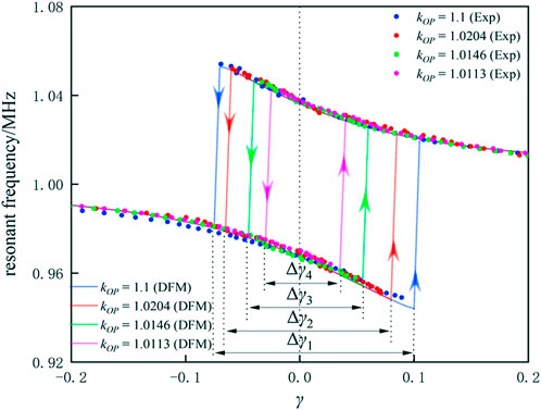
FIGURE 10. Effects of kOP on frequency hopping.
When frequency bifurcation occurs in the strong coupling region of a system, the two resonant frequency branches are equivalent. Therefore, when the system begins to oscillate, the selected operating frequency is determined by the asymmetry of the initial conditions. This situation is known as symmetry-breaking solution. The asymmetry of the initial conditions in an NPTS-WPT system refers to the random noise, glitches and numerous external disturbances that occur in the circuits at the moment that the system is powered on. These factors play important roles in the frequency selection process when the system oscillation begins. The initial operating frequency is normally random and uncontrollable. However, as can be observed from the analysis in Sections 3.2 and 3.3 indicates that, the system can be controlled to hop from the original resonant frequency point to another such point through the artificial detuning adjustment of the Rx circuit performed when the system runs steadily. Furthermore, the system can return to its original resonant frequency point through external rational induction. Therefore, the resonant frequency branch in a strong coupling region is selectable and controllable.
We illustrate the resonant frequency selection and control method is illustrated by using the example of the frequency-hopping curve (κ = 0.073) shown in Figure 11. When the system started, then either ω10 or ω30 was selected randomly as the operating frequency. Without loss of generality, we assumed the system to be running at the low frequency ω10. By using the external control circuit, γ was increased sharply while γ > γ2. For example, if we let γ = γ4 and then reset γ to zero, the system ran at the frequency ω30 because when γ > γ2, only the high-frequency branch remained in the system; i.e., this is the only choice. Subsequently, the value of γ decreased, and because of the inertia of the frequency variation, the system reached ω30 along the high-frequency branch. Similar behavior was observed when the system started in the case where it was assumed to be running at the high frequency ω30. By using the external control circuit, γ was reduced sharply and the inequality γ < γ1 was ensured. When γ = γ3 and γ was reset to zero, the system ran at the low frequency ω10. When the system originally operated at the low frequency ω10 during the aforementioned adjustment, γ decreased at a specific time, and regardless of how much γ decreased, the system operated at the low frequency ω10 after γ returned to zero. Similarly, when the system originally operated at the high frequency ω30 and γ was increased at a specific moment, the system will then run at the high frequency ω30 after γ returns to zero, regardless of how much γ increased. In summary, regardless of whether the system runs at the low or high resonant frequency under the initial conditions, it will run at the high-frequency resonant frequency point provided that γ is sufficiently large, is increased sharply at a specific moment and its value later returns to zero. Similarly, the system will run at the low-frequency resonant frequency point provided that γ is sufficiently small, is reduced sharply at a specific moment and its value later returns to zero.
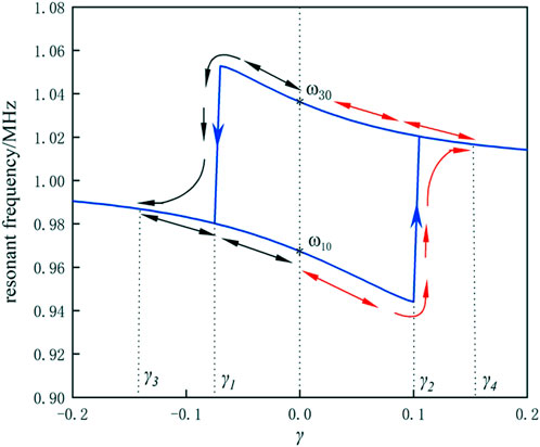
FIGURE 11. Frequency control principle.
To verify the correctness of the proposed control method, we designed a detuning control circuit for operation at the Rx to enable the system to select the designated resonant frequency branch to verify.
The operating parameters of the transfer system were consistent with those listed in Table 1. The distance between the Rx and Tx coils was set as 55 mm (i.e., κ=0.073) during the experiment. In this position, the system exhibited two resonant frequencies with theoretical values of 1.036 and 0.968 Mhz. Under the initial conditions, L2 = 8.79 μH, C2 = 2.88 nF and γ = 0. As shown in Figure 11, to ensure reliable frequency-hopping, we set cross point γ2 = 0.944 when γ was increasing and cross point γ1 = − 0.075 when γ was decreasing. Therefore, the adjustment of the equivalent inductance and capacitance values at the Rx circuit can be designed as shown in Figure 12. Regardless of whether the system was running on a low- or high-frequency resonance branch, when system oscillation began, it ran on the low-frequency branch according to Figure 11 when L2 switched from 8.79μH to 1.21 μH (i.e., when γ = − 0.20) and then switches back to 8.79 μH after 5 μs. The system will then run on the high-frequency branch when C2 switched from 2.88 nF to 11.03 nF (i.e., when γ = − 0.20) and then returned to 2.88 nF after 5 μs.
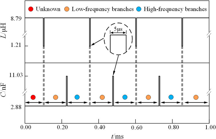
FIGURE 12. Variation in inductance and capacitance in the Rx circuit over time.
The above adjustment of the inductance and capacitance values of the Rx circuit was achieved using the circuit shown in Figure 13A. L2 and C2 enabled the natural frequency of the Rx loop to be consistent with that of the Tx loop. Switches S1 and S2 were disconnected from the circuit under normal operating conditions but were connected briefly when frequency-hopping was required. To switch between the equivalent inductance and capacitance values in the Rx circuit shown in Figure 12, the detuning control circuit parameters were configured as follows: L21 = 1.40 μH and C21 = 8.15 nF. Two pulses with a period of 250 μs and a peak pulse width of 5 μs are generated using the control module during the experiment to control the connection and disconnection of switches S1 and S2. The time interval between the two pulses was 120 μs. Figure 13B shows the experimental facility.
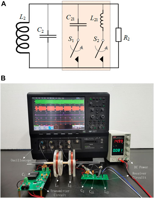
FIGURE 13. Resonant frequency control experiment: (A) Diagram of the detuning control circuit. (B) Experimental facilities.
Figure 14 presents the waveforms measured during the experiment. Switches S1 and S2 were connected for a short time and were disconnected later in the detuning control circuit to control the changes in the system operating frequency. When S1 was connected and then disconnected, the system ran on a high-frequency resonant branch; however, when switch S2 was connected and then disconnected, the system then ran on a low-frequency resonant branch. The operating frequencies of switches S1 and S2 were stabilized at 0.998 and 0.942 Mhz, respectively. The results for resonant frequency-hopping and selection were consistent with those from the theoretical analysis. When the detuning switches S1 and S2 were each connected for 5 μs, resonant frequency-hopping was induced successfully, thus indicating that the time required to induce the detuning is short. When S1 and S2 were connected, the Rx circuit received little power because of loop detuning, but the amplitude fluctuation at the Tx circuit is insignificant. After the system ran steadily at each of the two resonant frequency points, a considerable difference was observed in the voltage amplitude in the Rx circuit. When the Rx circuit ran at the high resonant frequency in the present system, the voltage amplitude at the coil end is higher. Therefore, the system could be controlled to run on the designated resonant frequency branch to obtain the optimal transfer performance by using the proposed resonant frequency control technology. Therefore, the experimental results verified the correctness of the frequency-hopping theory and the effectiveness of the proposed control method.
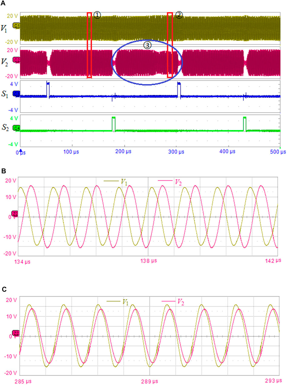
FIGURE 14. (A) Frequency-hopping test waveforms. The system is controlled to run on the high-frequency branch (B) or the low-frequency branch (C).
In the frequency control experiment shown in Figure 14, the stabilized system ran on the designated resonant frequency branch after the operation of the detuning switches S1 and S2. However, the frequency-hopping behavior was not synchronized with the detuning switch operation. A delay in hopping was observed, particularly when hopping from a high-to a low-frequency branch. As can be seen from the waveforms for case ③ in Figure 14A, the amplitudes of the front and rear waveforms differed considerably. After S2 was connected and then disconnected from the circuit, the system continued to run on the high-frequency resonant branch for a while before hopping to the low-frequency resonant branch. The transient waveforms before and after frequency-hopping were analyzed further, and Figure 15 shows the stretched-out waveform views before and after the actions of switches S1 and S2. Under these transmission conditions, S1 was connected and then disconnected from the circuit. It took approximately 7 μs for the Rx and Tx circuits to make the required adjustment before the system transit from the low-to the high-frequency resonance. After S2 was connected and then disconnected from the circuit, the Tx and Rx circuits exhibited delays of approximately 68 and 73 μs, respectively, to transit from the high-to the low-frequency resonance. The test results obtained for the distance between the Rx and Tx ends as 30, 40, 50 and 55 mm are presented in Table 2. From the data in the table, it can be seen that there was a delay in frequency-hopping at different distances. The low-frequency to high-frequency hopping delay was generally smaller than the high-frequency to low-frequency delay, and the hopping delay at the Tx end was slightly smaller than the hopping delay at the Rx end. The frequency jump process began with the closure of the detuning switch, causing the Rx end to become detuned, thereby inducing a change in the operating state of the Tx end. After oscillation adjustment, the Tx end completed the frequency jump, and the Rx end was coupled through electromagnetic induction before adjusting to a new resonant frequency branch for operation. Therefore, the delay time at the sending end was smaller than the delay time at the Rx end. In addition, we attempted to change the closing time of detuning switches S1 and S2 from 5 to 3 μs, observed that the system achieved frequency-hopping control, indicating that a shorter detuning time can induce frequency-hopping. However, the reason for the longer delay of high-frequency to low-frequency jumps requires further theoretical analysis in the future.
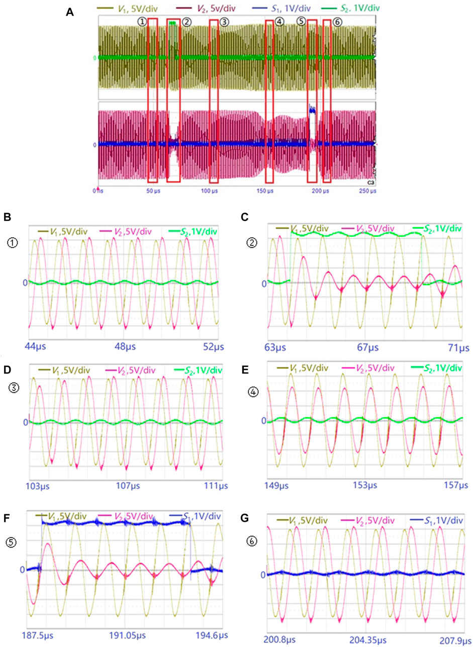
FIGURE 15. Image (A) is the frequency hopping waveforms. Images (B–G) are the transient waveforms of ①-⑥. Images (B) (D) and (G) show the system operates at high frequency, and Image (E) shows the system operates at low frequency. Switches S1 (F) and S2 (C) are connected for 5 μs and are disconnected later, respectively. The existence of ③ illustrates the Tx and Rx circuits require delays hopping between frequencies.
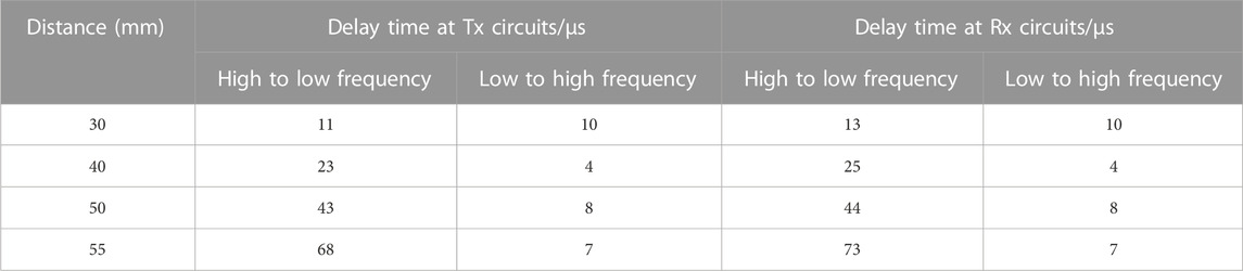
TABLE 2. Delay times of frequency-hopping.
In this study, the DFM was used to model and analyze the dynamics of NPTS-WPT systems. Resonant frequency-hopping was analyzed, and it was found that resonant frequency-hopping can be induced through system detuning occurring as a result of a change in the natural frequency of the Rx loop. Larger values of the coupling coefficient and the amplification factor of the OP amp produce a higher detuning tolerance and enable the system to maintain the original operating frequency branch without hopping stronger. Based on the evolution and hopping law of the resonant frequency, we proposed a frequency selection and control method. The system operating frequency can be induced to hop from one resonant frequency to another by adding a detuning control circuit to the Rx loop, which adjusts the equivalent inductance or capacitance as required at the Rx circuit. Finally, the experimental NPTS-WPT frequency-hopping device was designed. The experimental results demonstrated that a short detuning time successfully induces frequency-hopping and also show that there is a delay in the frequency-hopping process when compared with the control process. This also verifies the correctness of the frequency-hopping theory and the feasibility of the proposed control method. Therefore, the proposed frequency control method realizes the improvement of the operating frequency point from random selection previous studies to artificial directional selection and control under the condition of resonant frequency bifurcation.
The original contributions presented in the study are included in the article/Supplementary Material; further inquiries can be directed to the corresponding author.
CL is responsible for model establishment and analysis, and WD is responsible for conceptualization and visualization, HM is responsible for data curation, CZ is responsible for writing - original draft. All authors contributed to the article and approved the submitted version.
This work was supported in part by the National Natural Science Foundation of China under Grant 61403201.
Author WD was employed by Jiangsu Genture Electronic Information Co, Ltd.
The remaining authors declare that the research was conducted in the absence of any commercial or financial relationships that could be construed as a potential conflict of interest.
The Reviewer ZX declared a shared affiliation with the author CL, WD, HM, CZ at the time of the review.
All claims expressed in this article are solely those of the authors and do not necessarily represent those of their affiliated organizations, or those of the publisher, the editors and the reviewers. Any product that may be evaluated in this article, or claim that may be made by its manufacturer, is not guaranteed or endorsed by the publisher.
Abdelatty, O., Wang, X. Y., and Mortazawi, A. (2019). Position-insensitive wireless power transfer based on nonlinear resonant circuits. IEEE Trans. Microw. Theory Techn. 67, 3844–3855. doi:10.1109/tmtt.2019.2904233
Assawaworrarit, S., and Fan, S. (2020b). Efficient and robust wireless power transfer based on parity-time symmetry. AIP Conf. Proc. 2300 (1), 020005. doi:10.1063/5.0031691
Assawaworrarit, S., and Fan, S. H. (2020a). Robust and efficient wireless power transfer using a switch-mode implementation of a nonlinear parity-time symmetric circuit. Nat. Electron. 3, 273–279. doi:10.1038/s41928-020-0399-7
Assawaworrarit, S., Yu, X. F., and Fan, S. H. (2017). Robust wireless power transfer using a nonlinear parity–time-symmetric circuit. Nature 546, 387–390. doi:10.1038/nature22404
Cao, W., Wang, C., Chen, W., Hu, S., Wang, H., Yang, L., et al. (2022). Fully integrated parity–time-symmetric electronics. Nat. Nanotechnol. 17, 262–268. doi:10.1038/s41565-021-01038-4
Dong, W. J., Li, C. S., Zhang, H., and Ding, L. B. (2019b). Wireless power transfer based on current non-linear PT-symmetry principle. IET Power Electron 12, 1783–1791. doi:10.1049/iet-pel.2018.5937
Dong, W. J., Zhang, H., Li, C. S., and Liao, X. (2019a). Research on variable gap wireless energy transmission method for fuzes based on nonlinear PT symmetry principle. Acta Armamentarii 40, 35.
Engelberg, S. (2002). Limitations of the describing function for limit cycle prediction. IEEE Trans. Autom. Control 47, 1887–1890. doi:10.1109/tac.2002.804473
Hu, Z., Zeng, Z., Tang, J., and Luo, X. B. (2022). Quasi-parity-time symmetric dynamics in periodically driven two-level non-Hermitian system. [J] J. Phys. 71 (7), 074207–75186. doi:10.7498/aps.70.20220270
Hua, Z., Chau, K. T., Liu, W., and Tian, X. (2022). Pulse frequency modulation for parity-time-symmetric wireless power transfer system. IEEE Trans. Magnetics 58 (8), 1–5. Art no. 8002005. doi:10.1109/TMAG.2022.3153499
Ishida, H., Furukawa, H., and Kyoden, T. (2021). Scheme for providing parity-time symmetry for low-frequency wireless power transfer below 20 kHz. Electr. Eng. 103, 35–42. doi:10.1007/s00202-020-01041-3
Li, C. S., Dong, W. J., Ding, L. B., Zhang, H., and Sun, H. (2020). Transfer characteristics of the nonlinear parity-time-symmetric wireless power transfer system at detuning. Energies 13, 5175. doi:10.3390/en13195175
Li, J., and Huang, Y. (2022). Influence analysis of metal foreign objects on the wireless power transmission system. Front. Electron. 3, 2022. doi:10.3389/felec.2022.1033016
Liu F, F., Chowkwale, B., Jayathurathnage, P., and Tretyakov, S. (2019). Pulsed self-oscillating nonlinear systems for robust wireless power transfer. Phys. Rev. Appl. 12, 054040. doi:10.1103/physrevapplied.12.054040
Liu, G. J., and Zhang, B. (2018). Dual-coupled robust wireless power transfer based on parity-time-symmetric model. Chin. J. Elect. Eng. 4, 50.
Liu, J., Min, Y., Gao, J., Yang, A., and Zhou, J. (2022). Design and optimization of a modular wireless power system based on multiple transmitters and multiple receivers architecture. Front. Energy Res. 10. doi:10.3389/fenrg.2022.896575
Liu M, M., Chan, K. W., Hu, J. F., Lin, Q. F., Liu, J. W., and Xu, W. Z. (2019). Design and realization of a coreless and magnetless electric motor using magnetic resonant coupling technology. IEEE Trans. Energy Convers. 34, 1200–1212. doi:10.1109/tec.2019.2894865
Nguyen, H., and Agbinya, J. (2015). Splitting frequency diversity in wireless power transmission. IEEE Trans. Power Electron. 30, 6088–6096. doi:10.1109/tpel.2015.2424312
Ra’di, Y., Chowkwale, B., Valagiannopoulos, C., Liu, F., Alù, A., Simovski, C. R., et al. (2018). On-site wireless power generation. IEEE Trans. Antennas Propag. 66, 4260–4268. doi:10.1109/tap.2018.2835560
Shu, X. J., and Zhang, B. (2018). Single-wire electric-field coupling power transmission using nonlinear parity-time-symmetric model with coupled-mode theory. Energies 11, 532. doi:10.3390/en11030532
Sinha, M., Poon, J., Johnson, B., Rodriguez, M., and Dhople, S. (2018). Decentralized interleaving of parallel-connected buck converters. IEEE Trans. Power Electron. 34, 4993–5006. doi:10.1109/tpel.2018.2868756
Song, J., Yang, F. Q., Guo, Z. W., Wu, X., Zhu, K. J., JiangSun, J. Y., et al. (2021). Wireless power transfer via topological modes in dimer chains. Phys. Rev. Appl. 15, 014009. doi:10.1103/physrevapplied.15.014009
Tang, Y., Liang, C., and Liu, Y. (2022). Research progress of parity-time symmetry and anti-symmetry. [J] J. Phys. 71 (17), 171101–171123. doi:10.7498/aps.71.20221323
Truong, B. (2021). Further results on “design guidelines to avoid bifurcation in a series–series compensated IPTS”: Theoretical analysis and experimental validations. IEEE Trans. Ind. Electron. 68, 3643–3648. doi:10.1109/tie.2020.2978715
Wang, W., Duan, M., Zeng, Z., Liu, H., and Ji, Z. (2023). Research on optimal coil configuration scheme of insulator relay WPT system. Front. Electron. 4, 2023. doi:10.3389/felec.2023.1034082
Yang, D., Lin, Q., Li, X., and Cai, L. (2022). Efficiency and power of the parity-time-symmetric circuit for wireless power transfer. J. Electr. Eng. Technol. 17, 3355–3362. doi:10.1007/s42835-022-01095-2
Yatsugi, K., Oishi, K., and Iizuka, H. (2021). Ringing suppression of SiC MOSFET using a strongly coupled external resonator through analogy with passive PT-symmetry. IEEE Trans. Power Electron. 36, 2964–2970. doi:10.1109/tpel.2020.3013399
Zhang, Z. Q. (2020). Fractional-order time-sharing-control-based wireless power supply for multiple appliances in intelligent building. J. Ad. Res. 25, 227–234. doi:10.1016/j.jare.2020.04.013
Zhou, B. B., Deng, W. J., Wang, L. F., Dong, L., and Huang, Q. A. (2020). Enhancing the remote distance of LC passive wireless sensors by parity-time symmetry breaking. Phys. Rev. Appl. 13, 064022. doi:10.1103/physrevapplied.13.064022
Keywords: wireless power transfer, nonlinear parity-time symmetry, frequency bifurcation, frequency hopping, frequency control
Citation: Li C, Dong W, Ma H and Zhu C (2023) Frequency-hopping mechanism and control method for nonlinear parity-time-symmetric wireless power transfer systems. Front. Energy Res. 11:1174301. doi: 10.3389/fenrg.2023.1174301
Received: 28 February 2023; Accepted: 05 June 2023;
Published: 14 June 2023.
Edited by:
Jaber Abu Qahouq, University of Alabama, United StatesReviewed by:
Zhou Xiaodong, Army Engineering University of PLA, ChinaCopyright © 2023 Li, Dong, Ma and Zhu. This is an open-access article distributed under the terms of the Creative Commons Attribution License (CC BY). The use, distribution or reproduction in other forums is permitted, provided the original author(s) and the copyright owner(s) are credited and that the original publication in this journal is cited, in accordance with accepted academic practice. No use, distribution or reproduction is permitted which does not comply with these terms.
*Correspondence: Changsheng Li, bGljaGFuZ3NoZW5nMTk4NEBuanVzdC5lZHUuY24=
Disclaimer: All claims expressed in this article are solely those of the authors and do not necessarily represent those of their affiliated organizations, or those of the publisher, the editors and the reviewers. Any product that may be evaluated in this article or claim that may be made by its manufacturer is not guaranteed or endorsed by the publisher.
Research integrity at Frontiers
Learn more about the work of our research integrity team to safeguard the quality of each article we publish.