Two-stage robust optimization of regional integrated energy systems considering uncertainties of distributed energy stations

For a regional integrated energy system (RIES) composed of an energy supply network and distributed energy station, the uncertainty of distributed photovoltaic (PV) output and the fluctuation of various loads pose significant challenges to the stability of system operation and the accuracy of optimal scheduling. In order to enhance the operational reliability of regional integrated energy systems and reduce the impact of photovoltaic and load uncertainties on distributed energy stations, this study proposes robust optimization method of regional integrated energy systems that takes into account the uncertainty of the distributed energy station. First, the regional integrated energy system is divided into an upper electric-gas energy supply network and a lower distributed energy station. The upper model mainly realizes energy transmission, while the lower model is a two-stage robust optimization model of distributed energy stations in the form of min–max–min, which mainly realizes flexible energy supply of different types of energy. Then, the lower two-stage robust optimization model is simplified and solved using a column and constraint generation (CCG) algorithm. After that, an alternating direction method of multipliers (ADMM) is used to solve the upper and lower models of the regional integrated energy system, and the solution scale is reduced while ensuring the correlation between the energy transmission network and the distributed energy stations. Finally, a test example is provided to illustrate the effectiveness and usefulness of the proposed method. It follows from simulation results that the robust optimization method can effectively reduce the instability of the system operation caused by uncertainty factors and improve the system’s anti-interference ability, and in addition, systems with high penetration levels of photovoltaic output will benefit more from robust optimization.

1 Introduction

In order to comply with the world’s green and low-carbon development trend, it has become particularly significant to promote the integration of sources, networks, loads, and storage and to build a multi-energy-coupled regional integrated energy system (RIES). In addition to the exploration and research of new energy sources, the improvement of the energy supply form is also of equal significance (Zhao et al., 2022a). The role of the regional integrated energy system, as a promising solution of bearing energy for human society in the future, is rapidly developing in the field of efficient energy utilization, energy conservation, renewable energy consumption, and emission reduction (Balsamo et al., 2020). Followed by the foundation of the RIES concept, countries worldwide have responded positively and vigorously by carrying out extensive research on the RIES (Zhang et al., 2022). Some key issues of the RIES have already been studied from various perspectives in China (Zhang et al., 2020; Zhou and Zhang, 2020; Zhao et al., 2022b; Rezaei et al., 2022; Yang et al., 2022), and many theoretical and practical results have been obtained.

A RIES can fully exploit the complementary characteristics of multiple energy sources to achieve multi-layer energy efficiency, which could also reduce operating costs and carbon emissions effectively, and further consume renewable energy that cannot be consumed by traditional single energy systems through the conversion between different energy sources (Sioshansi et al., 2021). However, a RIES is much more complex than the traditional energy system and has various coupling forms, which need higher requirements on optimization and planning techniques (Wang et al., 2022). In the study by Li et al. (2021a), a second-order cone method for a RIES with electricity–gas interconnection was proposed, by which the non-convex electricity–gas optimal power flow model was transformed into a convex optimization model, and the scaling degree was limited by setting a penalty term, which increases the model convergence. In the study by Li et al. (2022a), an energy network was modeled in matrix form, where energy conversion and coupling could be described by the network graph theory, and the complexity of the optimization operation could be reduced. In the study by Li et al. (2021b), a method for the optimal design of RIES partitions was proposed by combining the K-means and genetic algorithm, by which the local resource data were clustered to evaluate the availability of all resources. In the study by Li et al. (2022b), an improved third-order quantized state system (QSS) method was proposed for the simulation of a district heating system (DHS) by combining a quantized state system and time-discrete integration. In the study by Zhu et al. (2022), a dynamic programming algorithm was introduced to replace a multi-stage decision problem with a series of single-stage sub-problems to obtain the global optimal scheduling solution. It is pointed out that the aforementioned results investigate the optimization of the RIES from several aspects. Nevertheless, few results study the operating characteristics and solution methods after the distributed energy station (DES) is connected, where the influences of its uncertainty factors on the system are not sufficiently considered.

On the other hand, the uncertainties of various loads and renewable energy sources seriously affect the safe and reliable operation of the RIES (Wang et al., 2020), which is an important problem that cannot be ignored in the optimal operation process of the RIES. In the study by Xu et al. (2022), an efficient wind speed prediction model based on phase space reconstruction and BLS was proposed, which could evaluate the regularity of wind speed effectively without the overfitting issue. In the study by Xiang et al. (2021), an uncertainty model was proposed for the integrated demand response (IDR) of energy prices based on fuzzy and probabilistic variables. In the study by Feng et al. (2018), based on the imprecise Dirichlet model (IDM), a non-parametric fuzzy set of wind power output distribution probabilities was obtained from historical data and used in the uncertainty optimization of the RIES. In the study by Wang et al. (2017), chance-constrained objective planning was structured to model wind power uncertainty, and the developed results could guarantee the reliability of the system under a certain probability of satisfaction. Furthermore, based on the aforementioned probabilistic models (Wang et al., 2017; Feng et al., 2018), the probabilities were dealt with using the point estimation method, and the objective function was then set as the expected value in Li et al.’s (2021a) study. In the study by Li et al. (2022c), an optimal scheduling strategy of an IDR-enabled RIES in uncertain environments was proposed to improve the flexibility of system operation and the comprehensive satisfaction of users, while battery degradation, electric vehicles’ interaction, and load uncertainty were ignored. In the study by Fu et al. (2021), a two-stage stochastic programming model was proposed to deal with the uncertainty of PV generation and energy demand in the RIES. However, the aforementioned models deal with uncertainties that are all based on probabilities and rely on the distribution models with uncertain parameters. However, in some cases, the actual operation results have a certain probability of constraint violation; therefore, the robust optimization methods are expected to be used to solve these issues effectively.

Based on the aforementioned discussions, for the RIES containing a DES, it is necessary and important to take the uncertainties of the DES into consideration and thoroughly investigate its optimal and analyzing methods. Hence, in this paper, the robust optimization of the RIES considering the uncertainties of the DES will be discussed in detail. First, the overall model is divided into two layers according to their specific functions: the energy supply network (ESN) is set as the upper-layer model, and the DES is set as the lower-layer model. Second, the lower-layer DES model is formulated as a two-stage robust optimization model in the form of “min–max–min,” and it is split into two parts: a main problem and a sub-problem. Then, the column and constraint generation (CCG) algorithm (Zeng and Zhao, 2013) is applied to iteratively solve these two problems in the lower-layer DES model. Finally, considering the correlation between the upper-layer ESN model and the lower-layer DES model, the alternating direction method of multipliers (ADMM) (Sun et al., 2018) is used to solve the overall model. The main innovative contributions of this paper are summarized as follows:

(1) A two-layer model of the RIES is constructed innovatively according to the functions of each section of the model, where the electricity–gas transmission network model is taken as the upper-layer model and the multi-energy coupled distributed energy station is taken as the lower-layer model.

(2) The two-stage robust optimization method is applied to matrix the lower-layer model, which can dramatically enhance the stability of the RIES to resist the uncertainty of the photovoltaic and load. More importantly, it can be easily solved using the CCG algorithm.

(3) The ADMM algorithm is used to solve the RIES with distributed energy stations, which can largely reduce the solving difficulty in an iterative way, where a connection between the upper- and lower-layer models is established.

The remaining sections of this paper are arranged as follows: Sections 2 and Sections 3 present the mathematical models of the upper-layer ESN and lower-layer DES which include a two-stage robust optimization equivalent model with its constraints and objective functions, respectively. Section 4 describes the solving methods used to solve the proposed model, whereas the simulation example and obtained results are demonstrated and discussed in Section 5. Finally, the conclusions are drawn in Section 6.

2 Upper-layer energy supply network model

The ESN is the upper layer of the RIES, which plays the role of connecting various energy-using nodes and supplying energy to the lower-layer DES. Heat is transmitted in the form of water flow, and the energy loss is serious when the transmission distance is long. Moreover, the time lag phenomenon of heat is more notable than that of electricity and gas. Since the heat transmission network has evident disadvantages compared with electricity and gas transmission networks, the RIES studied in this paper only considers electricity and gas transmission networks, while the heat transmission network is not considered.

2.1 Steady-state model of the power system

The power flow equation of radial distribution networks is formulated as follows (Farivar and Low, 2013a):

$\left\{\begin{array}{l}{P}_j^t={\displaystyle \sum }_{l\in m\left(j\right)}{P}_{jl}^t-{\displaystyle \sum }_{l\in n\left(j\right)}\left[P_{ij}^t-R_{ij}{\left(I_{ij}^t\right)}^2\right]\\ Q_j^t={\displaystyle \sum }_{l\in m\left(j\right)}{Q}_{jl}^t-{\displaystyle \sum }_{l\in n\left(j\right)}\left[Q_{ij}^t-X_{ij}{\left(I_{ij}^t\right)}^2\right]\end{array}\right.,(1)$

where $P_j^t$ and $Q_j^t$ denote the active and reactive powers, respectively, injected into node $j$ at time $t$; $P_{jl}^t$ and $Q_{jl}^t$ are the active and reactive powers, respectively, flowing from node $j$ to node $l$ at time $t$; $R_{ij}$ and $X_{ij}$ are the resistance and reactance, respectively, of line $ij$; $I_{ij}^t$ is the current flowing through line $ij$ at time $t$; $n\left(j\right)$ is the set of sending nodes with node $j$ as the end node; and $m\left(j\right)$ is the set of the end nodes with node $j$ as the sending node.

In addition, the relationship between the current $I_{ij}^t$ flowing through line $ij$ and the node voltage is given as follows:

${\left(U_i^t\right)}^2-{\left(U_j^t\right)}^2=2\left(R_{ij}{P}_{ij}^t+X_{ij}{Q}_{ij}^t\right)-{\left(I_{ij}^t\right)}^2{\left(R_{ij}\right)}^2-{\left(I_{ij}^t\right)}^2{\left(X_{ij}\right)}^2,(2)$

${\left(I_{ij}^t\right)}^2{\left(U_i^t\right)}^2={\left(P_{ij}^t\right)}^2+{\left(Q_{ij}^t\right)}^2,(3)$

where $U_i^t$ is the voltage of node $i$ at time $t$.

In the process of transmitting power in the distribution network, reactive power compensation can effectively improve the power factor and reduce line losses. Common reactive power compensation devices include continuous-type Static Var Generators (SVG) and discrete-type capacitors (CP), where CP satisfies

$Q_{\mathrm{C}\mathrm{P}}^t=Q_{\mathrm{C}\mathrm{P},\mathrm{U}}{\displaystyle \sum }_{m=1}^M{\theta }_{\mathrm{C}\mathrm{P},m}^t,(4)$

${\theta }_{\mathrm{C}\mathrm{P},m}^t>={\theta }_{\mathrm{C}\mathrm{P},m+1}^t(5)$

${\theta }_{\mathrm{C}\mathrm{P}\_\mathrm{a}\mathrm{d}\mathrm{d}}^t+{\theta }_{\mathrm{C}\mathrm{P}\_\mathrm{d}\mathrm{e}\mathrm{l}}^t<=1(6)$

${\displaystyle \sum }_{t=1}^T\left({\theta }_{\mathrm{C}\mathrm{P}\_\mathrm{a}\mathrm{d}\mathrm{d}}^t+{\theta }_{\mathrm{C}\mathrm{P}\_\mathrm{d}\mathrm{e}\mathrm{l}}^t\right)<={\theta }_{\max }(7)$

${\displaystyle \sum }_{m=1}^M{\theta }_{\mathrm{C}\mathrm{P},m}^{t+1}-{\displaystyle \sum }_{m=1}^M{\theta }_{\mathrm{C}\mathrm{P},m}^t\le \mathrm{\gamma }{\theta }_{\mathrm{C}\mathrm{P}\_\mathrm{a}\mathrm{d}\mathrm{d}}^t-{\theta }_{\mathrm{C}\mathrm{P}\_\mathrm{d}\mathrm{e}\mathrm{l}}^t,(8)$

${\displaystyle \sum }_{m=1}^M{\theta }_{\mathrm{C}\mathrm{P},m}^{t+1}-{\displaystyle \sum }_{m=1}^M{\theta }_{\mathrm{C}\mathrm{P},m}^t\ge {\theta }_{\mathrm{C}\mathrm{P}\_\mathrm{a}\mathrm{d}\mathrm{d}}^t-\mathrm{\gamma }{\theta }_{\mathrm{C}\mathrm{P}\_\mathrm{d}\mathrm{e}\mathrm{l}}^t,(9)$

where $Q_{\mathrm{C}\mathrm{P}}^t$ is the compensated reactive power of the CP at time $t$; $Q_{\mathrm{C}\mathrm{P},\mathrm{U}}$ is the reactive power output corresponding to each step of the CP; ${\theta }_{\mathrm{C}\mathrm{P},m}^t$, ${\theta }_{\mathrm{C}\mathrm{P}\_\mathrm{a}\mathrm{d}\mathrm{d}}^t$, and ${\theta }_{\mathrm{C}\mathrm{P}\_\mathrm{d}\mathrm{e}\mathrm{l}}^t$ denote the 0–1 variables at time $t$; $\mathrm{\gamma }$ is the maximum number of steps that can be adjusted; and ${\theta }_{\max }$ is the maximum number of adjustments per day.

It should be pointed out that in Eq. 4, a 0–1 variable is set for each grade, and the sum of each grade is the current grade. Equation 5 limits the gears to incremental steps, and it is not possible to have a high gear of 1 and a low gear of 0. Equation 6 ensures that the increase and decrease of gears cannot occur simultaneously, and Eq. 7 shows that the number of gear adjustments per day is limited. Equations 8, 9 together restrict the upward or downward adjustment of gears to the maximum adjustment range of gears.

For the SVG, the model is simpler than the CP and satisfies

$Q_{\mathrm{S}\mathrm{V}\mathrm{G}}^{\min }\le Q_{\mathrm{S}\mathrm{V}\mathrm{G}}^t\le Q_{\mathrm{S}\mathrm{V}\mathrm{G}}^{\max },(10)$

where $Q_{\mathrm{S}\mathrm{V}\mathrm{G}}^{\min }$ and $Q_{\mathrm{S}\mathrm{V}\mathrm{G}}^{\max }$ are the lower and upper limits of the regulation range, respectively, and $Q_{\mathrm{S}\mathrm{V}\mathrm{G}}^t$ is the reactive power of the SVG at time $t$.

The input and output energy of a power system should satisfy the law of energy conservation, so the following relationship should be ensured:

$\left\{\begin{array}{l}{Q}_j^t+Q_{\mathrm{L},j}^t=Q_{\mathrm{S}\mathrm{V}\mathrm{G},j}^t+Q_{\mathrm{C}\mathrm{P},j}^t+Q_{\mathrm{G},j}^t,\\ P_j^t+P_{\mathrm{L},j}^t=P_{\mathrm{G},j}^t\end{array}\right.(11)$

where $Q_{\mathrm{L},j}^t$ and $P_{\mathrm{L},j}^t$ are the reactive and active loads of node $j$ at time $t$, respectively. $P_{\mathrm{G},j}^t$ and $Q_{\mathrm{G},j}^t$ are the active and reactive powers of the generator of node $j$ at time $t$, respectively.

2.2 Steady-state model of the gas system

The gas system is mainly composed of a gas source, gas transmission pipelines, a compressor, and loads, and the relationship between its flow and pressure is formulated as follows:

$f_q^t=M_q{\nu }_{mn}\sqrt{{\nu }_{mn}\left[{\left(p_m^t\right)}^2-{\left(p_n^t\right)}^2\right]}(12)$

$M_q=\varsigma \frac{18.73T_0{D}_q^{\frac{8}{3}}}{p_0\sqrt{G{L}_q{T}_{qa}{Z}_{qa}}}(13)$

${\nu }_{mn}=\left\{\begin{array}{l}1\\ -1\end{array}\right.\begin{array}{l}{p}_m^t-p_n^t\ge 0\\ p_m^t-p_n^t<0\end{array}(14)$

where $f_q^t$ is the flow of the pipe $q$ at time $t$, $p_m^t$ is the pressure of node $m$ at time $t$, $\varsigma$ represents the efficiency factor of the pipe $q$, $T_0$ is the standard temperature, $D_q$ denotes the inner diameter of the pipe $q$, $p_0$ is the standard pressure, $G$ is the gas relative density, $L_q$ is the length of the pipe $q$, $T_{qa}$ is the average temperature of the pipe $q$, and $Z_{qa}$ is the average compression factor of the pipe $q$.

There is a pressure loss during gas transmission, which needs to be replenished by a compressor. The gas flow to be consumed is formulated as

${\sigma }_u^t={\alpha }_u+{\beta }_u{P}_{\mathrm{c}\mathrm{o}\mathrm{m}}^t+{\gamma }_u{\left(P_{\mathrm{c}\mathrm{o}\mathrm{m}}^t\right)}^2(15)$

$\left.P_{\mathrm{c}\mathrm{o}\mathrm{m}}^t=G_u{f}_{com,u}{\left((\frac{p_m^t}{p_n^t}\right)}^{Z_u}-1\right)(16)$

where ${\sigma }_u^t$ is the gas flow consumed by the compressor $u$ at time $t$; ${\alpha }_u$, ${\beta }_u$, and ${\gamma }_u$ are the energy consumption coefficients of the compressor $u$; $P_{\mathrm{c}\mathrm{o}\mathrm{m}}^t$ denotes the gas energy consumed by the compressor $u$ at time $t$; $G_u$ is the coefficient related to temperature and efficiency; $f_{com,u}$ represents the flow through the compressor $u$ at time $t$; and $Z_u$ is the other compression factor.

Similar to the law of conservation of energy in electric power systems, the input and output of gas at each node in a gas system should be equal, which satisfies

$\left(A+U\right)f+\varpi -T\tau =0,(17)$

where $f$ denotes the branch flow vector, $\varpi$ is the node gas injection flow vector, $\tau$ is the compressor consumption flow vector, $A$ is the branch node association matrix, $U$ represents the unit node association matrix, and $T$ is the compressor node association matrix.

The power flow model and natural gas model is the non-convex and non-linear. In order to facilitate the subsequent solution, second-order cone scaling (Farivar and Low, 2013a; Farivar and Low, 2013b) is used to convert the distribution network and natural gas system models into the convex model.

2.3 The objective function of the upper-layer ESN

The operation of the upper-layer ESN is optimized by minimizing net costs as follows:

$\left\{\begin{array}{l}{C}_{up}={\displaystyle \sum }_{t=1}^T\left.{\left(a+b{P}_G^t+c(P_G^t\right)}^2+h{G}_G^t\right)-{\displaystyle \sum }_{t=1}^T\left(pric{e}_{\mathrm{e}}^t{P}_{\mathrm{g}\mathrm{r}\mathrm{i}\mathrm{d}}^t+pric{e}_{\mathrm{g}}^t{G}_{\mathrm{g}\mathrm{a}\mathrm{s}}^t\right)\\ P_G^t={\displaystyle \sum }_{k=1}^N{P}_{G,k}^t,G_G^t={\displaystyle \sum }_{k=1}^M{G}_{G,k}^t\\ obj=\min C_{up}\end{array}\right.,(18)$

where $a$, $b$, and $c$ denote the generators’ cost coefficients; $h$ is the cost coefficient of gas supply; $G_G^t$ is the gas supply quantity of the gas source at time $t$; $pric{e}_e^t$ and $pric{e}_g^t$ represent the purchase prices of electricity and gas of the lower-layer DES at time $t$, respectively; $P_{grid}^t$ and $P_{gas}^t$ are the purchased power and gas power of the lower-layer DES from the upper-layer ESN at time $t$, respectively; and $T$ is the dispatch period. $P_{G,k}^t$ and $G_{G,k}^t$ are the k-th generator and air source supply, respectively. $N$ and $M$ are the total number of generators and gas sources, respectively.

2.4 Other constraints

In the upper-layer ESN, upper- and lower-limit constraints should be added to the individual equipment output, voltage value, gas flow value, node pressure, and gas supply from the gas source, which are expressed uniformly by

${\mathrm{\Theta }}^{\min }\le {\mathrm{\Theta }}^t\le {\mathrm{\Theta }}^{\max },(19)$

where ${\mathrm{\Theta }}^{\min }$ and ${\mathrm{\Theta }}^{\max }$ are the lower and upper limits of the variable ${\mathrm{\Theta }}^t$, respectively. ${\mathrm{\Theta }}^t$ represents the variables such as equipment output, voltage value, gas flow value, node pressure, and gas supply from the gas source.

3 Lower-layer distributed energy station model

The DES can meet multiple energy demands of consumers and interconnect different types of energy sources through energy conversion equipment. In this study, the considered DES model includes two types of energy inputs, electricity and gas, and three types of energy loads, electricity, heat, and cooling. Moreover, energy conversion equipment includes gas turbine, gas boiler, absorption chiller, and electric chiller, while energy storage equipment includes electricity and heat storage, mainly considering the uncertainty of photovoltaic inside the DES and the uncertainties of the three loads.

3.1 Energy conversion equipment model

3.1.1 Gas boiler

The gas boiler can be modeled according to the following equation:

$H_{\mathrm{G}\mathrm{B}}^t=G_{\mathrm{G}\mathrm{B}}^t{\eta }_{\mathrm{G}\mathrm{B}},(20)$

where $H_{\mathrm{G}\mathrm{B}}^t$ and $G_{\mathrm{G}\mathrm{B}}^t$ are the heat production and gas consumption of the gas boiler at time $t$, respectively, and ${\eta }_{\mathrm{G}\mathrm{B}}$ is the heat production efficiency.

3.1.2 Gas turbine

The gas turbine is coupling equipment that contains electric, gas, and thermal devices with the following input–output relationship:

$\left\{\begin{array}{l}{P}_{\mathrm{G}\mathrm{T}}^t=G_{\mathrm{G}\mathrm{T}}^t{\eta }_{\mathrm{G}\mathrm{T}}\\ \lambda =\frac{P_{\mathrm{G}\mathrm{T}}^t}{H_{\mathrm{G}\mathrm{T}}^t}\end{array}\right.,(21)$

where $P_{\mathrm{G}\mathrm{T}}^t$ denotes the power production of the gas turbine at time $t$, $G_{\mathrm{G}\mathrm{T}}^t$ is the gas consumption of the gas turbine at time $t$, $H_{\mathrm{G}\mathrm{T}}^t$ represents the heat production of the gas turbine at time $t$, ${\eta }_{\mathrm{G}\mathrm{T}}$ is the power production efficiency, and $\lambda$ is the electricity-to-heat ratio.

3.1.3 Electric chiller

The electric chiller is mathematically expressed as

$C_{\mathrm{E}\mathrm{C}}^t=P_{\mathrm{E}\mathrm{C}}^{t}CO{P}_{\mathrm{E}\mathrm{C}},(22)$

where $C_{\mathrm{E}\mathrm{C}}^t$ and $P_{\mathrm{E}\mathrm{C}}^t$ are the cooling production and power consumption of the electric chiller at time $t$, respectively. $CO{P}_{\mathrm{E}\mathrm{C}}$ is the performance coefficient of the electric chiller.

3.1.4 Absorption chiller

The absorption chiller model is presented as follows:

$\left\{\begin{array}{l}{C}_{\mathrm{A}\mathrm{C}}^t=H_{\mathrm{A}\mathrm{C}}^{t}CO{P}_{\mathrm{A}\mathrm{C}}\\ CO{P}_{\mathrm{A}\mathrm{C}}=\frac{CO{P}_{\mathrm{A}\mathrm{C}}^0}{a_{\mathrm{A}\mathrm{C}}{\left({\beta }_{\mathrm{A}\mathrm{C}}\right)}^2+b_{\mathrm{A}\mathrm{C}}{\beta }_{\mathrm{A}\mathrm{C}}+c_{\mathrm{A}\mathrm{C}}}\end{array}\right.,(23)$

where $C_{\mathrm{A}\mathrm{C}}^t$ and $H_{\mathrm{A}\mathrm{C}}^t$ are the cooling production and heat consumption of the absorption chiller at time $t$, respectively; $CO{P}_{\mathrm{A}\mathrm{C}}$ is the performance coefficient of the absorption chiller; $CO{P}_{\mathrm{A}\mathrm{C}}^0$ is the rated conversion efficiency of the absorption chiller; and $a_{\mathrm{A}\mathrm{C}}$, $b_{\mathrm{A}\mathrm{C}}$, and $c_{\mathrm{A}\mathrm{C}}$ denote the conversion factors of the absorption chiller. ${\beta }_{\mathrm{A}\mathrm{C}}$ is the workload rate of the absorption chiller.

3.2 Energy storage equipment model

Energy storage equipment is modeled as

$E_i^t=E_i^{t-1}\left(1-{\delta }_i\right)+{\upsilon }_i{C}_i^t{\eta }_{i,char}-\frac{\left(1-{\upsilon }_i\right)D_i^t}{{\eta }_{i,dis}}(24)$

where $E_i^t$ is the reserves of energy storage at time $t$; $i$ is the type of energy storage device, which includes electricity and heat storage; ${\delta }_i$ is the self-loss rate of the energy storage device; $C_i^t$ and $D_i^t$ are the charging and discharging powers of the energy storage device, respectively; ${\eta }_{i,char}$ and ${\eta }_{i,dis}$ represent the charging and discharging efficiencies of the energy storage device, respectively; and ${\upsilon }_i$ is a 0–1 variable to represent the storage mode: 0 if discharging, and 1 if charging.

There are also various constraints on the energy storage device, for example, charging and discharging cannot be done simultaneously and the total energy storage remains unchanged in a scheduling cycle, in addition to upper and lower limits on variable parameters, which are formulated as

$\left\{\begin{array}{l}{C}_i^t\le {\upsilon }_i^t{C}_i^{\max }\\ D_i^t\le \left(1-{\upsilon }_i\right)D_i^{\max }\\ E_i^1=E_i^{24}\\ E_i^t\in \left[E_i^{\min },E_i^{\max }\right]\end{array}\right.(25)$

3.3 The model of uncertain parameters

PV and various load data are mainly derived by forecasting; however, there are always various random factors that affect the accuracy of forecasting in reality. Random factors cannot be avoided, and if they are not considered when developing the operation scheme, they may lead to inaccurate operation schemes and even cause operational accidents. To equip the system with a certain anti-interference ability and to ensure the system’s safe and reliable operation in different environments, it is necessary to deal with those uncertain parameters. The uncertainty $U$ model of PV output and load is given by

$U=\left\{\begin{array}{l}u=\left[u_{\mathrm{P}\mathrm{V}}^t,u_{i,\mathrm{L}}^t\right]\in {\mathbb{R}}^{\left(T\right)\times 4},t=\mathrm{1,2},\cdots ,T\\ u_{\mathrm{P}\mathrm{V}}^t={\widehat{u}}_{\mathrm{P}\mathrm{V}}^t-B_{\mathrm{P}\mathrm{V}}^t\Delta u_{\mathrm{P}\mathrm{V}}^{\max ,t}+D_{\mathrm{P}\mathrm{V}}^t\Delta u_{\mathrm{P}\mathrm{V}}^{\max ,t}\\ {\displaystyle \sum }_{t=1}^T\left(B_{\mathrm{P}\mathrm{V}}^t+D_{\mathrm{P}\mathrm{V}}^t\right)\le {\mathrm{\Gamma }}_{\mathrm{P}\mathrm{V}}\\ u_{i,\mathrm{L}}^t={\widehat{u}}_{i,\mathrm{L}}^t-B_{i,\mathrm{L}}^t\Delta u_{i,\mathrm{L}}^{\max ,t}+D_{i,\mathrm{L}}^t\Delta u_{i,\mathrm{L}}^{\max ,t}\\ {\displaystyle \sum }_{t=1}^T\left(B_{i,\mathrm{L}}^t+D_{i,\mathrm{L}}^t\right)\le {\mathrm{\Gamma }}_{i,\mathrm{L}}\end{array}\right.(26)$

where $u_{\mathrm{P}\mathrm{V}}^t$ and $u_{i,\mathrm{L}}^t$ are the uncertainty variables of PV output and load power at time $t$ after introducing uncertainty, respectively. ${\widehat{u}}_{\mathrm{P}\mathrm{V}}^t$ and ${\widehat{u}}_{i,\mathrm{L}}^t$ are the expected values of PV output and load power at time $t$, respectively. $\Delta u_{\mathrm{P}\mathrm{V}}^{\max ,t}$ and $\Delta u_{i,\mathrm{L}}^{\max ,t}$ denote the maximum allowable deviations of PV output and load power at time $t$, respectively; $i$ represents the energy types including electricity, heat, and cooling; and $B_{\mathrm{P}\mathrm{V}}^t$, $D_{\mathrm{P}\mathrm{V}}^t$, $B_{i,\mathrm{L}}^t$, and $D_{i,\mathrm{L}}^t$ are 0–1 variables, while ${\mathrm{\Gamma }}_{\mathrm{P}\mathrm{V}}$ and ${\mathrm{\Gamma }}_{i,\mathrm{L}}$ are the uncertainty conservativeness adjustment parameters.

3.4 Energy balance constraints

The lower-layer DES also needs to satisfy the energy conservation law, and the balance between the input and output quantities of each type of energy should be maintained as

$\left\{\begin{array}{l}{P}_{\mathrm{g}\mathrm{r}\mathrm{i}\mathrm{d}}^t+u_{\mathrm{P}\mathrm{V}}^t+P_{\mathrm{G}\mathrm{T}}^t+D_e^t=u_{e,\mathrm{L}}^t+C_e^t+P_{\mathrm{E}\mathrm{C}}^t\\ H_{\mathrm{G}\mathrm{T}}^t+H_{\mathrm{G}\mathrm{B}}^t+D_h^t=u_{h,\mathrm{L}}^t+C_h^t+P_{\mathrm{A}\mathrm{C}}^t\\ C_{\mathrm{E}\mathrm{C}}^t+C_{\mathrm{A}\mathrm{C}}^t=u_{c,\mathrm{L}}^t\\ G_{\mathrm{g}\mathrm{a}\mathrm{s}}^t=G_{\mathrm{G}\mathrm{T}}^t+G_{\mathrm{G}\mathrm{B}}^t\end{array}\right.,(27)$

where $D_e^t$, $C_e^t$, $D_h^t$, and $C_h^t$ are the variables of charging and discharging powers corresponding to the electric and thermal energies, respectively, while $u_{e,\mathrm{L}}^t$, $u_{h,\mathrm{L}}^t$, and $u_{c,\mathrm{L}}^t$ are the variables of load uncertainty corresponding to the electricity, heat, and cooling, respectively.

3.5 Upper- and lower-bound constraints

Like the upper layer, there are also some limit constraints on the output of each device in the lower layer, which are omitted here due to the length of the paper.

3.6 The objective function of the lower-layer DES

After presenting the mathematical models of both layers, the following objective function can be formulated:

$\left\{\begin{array}{l}{C}_{dn}={\displaystyle \sum }_{t=1}^T\left(pric{e}_{\mathrm{e}}^t{P}_{\mathrm{g}\mathrm{r}\mathrm{i}\mathrm{d}}^t+pric{e}_{\mathrm{g}}^t{G}_{\mathrm{g}\mathrm{a}\mathrm{s}}^t\right)\\ obj=\underset{x}{\min }\underset{u\in U}{\max }\underset{y\in \mathrm{\Omega }\left(x,u\right)}{\min }{C}_{dn}\\ x=\left[{\upsilon }_i^t,C_i^t,D_i^t,E_i^t\right]\\ y=\left[P_{\mathrm{g}\mathrm{r}\mathrm{i}\mathrm{d}}^t,G_{\mathrm{g}\mathrm{a}\mathrm{s}}^t,G_{\mathrm{G}\mathrm{T}}^t,P_{\mathrm{G}\mathrm{T}}^t,H_{\mathrm{G}\mathrm{T}}^t,G_{\mathrm{G}\mathrm{B}}^t,H_{\mathrm{G}\mathrm{B}}^t,H_{\mathrm{A}\mathrm{C}}^t,C_{\mathrm{A}\mathrm{C}}^t,P_{\mathrm{E}\mathrm{C}}^t,C_{\mathrm{E}\mathrm{C}}^t\right]\end{array}\right..(28)$

To facilitate subsequent simplification and solution, the lower-layer DES model is written in a matrix compact form:

$\begin{array}{l}\underset{x}{\min }\underset{u\in U}{\max }\underset{y\in \mathrm{\Omega }\left(x,u\right)}{\min }{C}^{\mathrm{T}}y\\ \mathrm{s}.\mathrm{t}.Dy\ge d\\ Ly+Tx=0\\ I_{u}y=u\\ Px=p\\ Fx\ge f\end{array}.(29)$

The objective function can be split into two stages: the first stage is to optimize the charging and discharging behavior of the power and heat storage equipment, called the main problem (MP), and the second stage is to search for the optimal equipment output and energy purchased under the worst uncertain parameters, called the sub-problem (SP). Uncertainty is expressed by the box uncertainty set. The sub-problem is to solve the worst scenario in the interval according to the conservatism parameter and complete the two-stage robust optimization together with the main problem. The main problem and sub-problem of the objective function are described as follows:

$\begin{array}{l}\mathrm{M}\mathrm{P}:\\ \underset{x}{\min }\sigma \\ \mathrm{s}.\mathrm{t}.Dy\ge d\\ Ly+Tx=0\\ I_{u}y=u\\ Px=p\\ Fx\ge f\\ \sigma \ge Cy\end{array},(30)$

$\begin{array}{l}\mathrm{S}\mathrm{P}:\\ Q\left(x\right)=\underset{u\in U}{\max }\underset{y\in \mathrm{\Omega }\left(x,u\right)}{\min }{C}^{\mathrm{T}}y\\ \mathrm{s}.\mathrm{t}.Dy\ge d\\ Ly+Tx=0\\ I_{u}y=u\end{array}.(31)$

The sub-problem is a max–min type problem, which is not easy to solve. By the strong dual principle, the inner min problem can be converted into a max problem and merged with the outer one to obtain the following form of the sub-problem (Ding et al., 2016):

$\begin{array}{l}\mathrm{S}\mathrm{P}:\\ Q\left(x\right)=\underset{u\in U,\omega }{\max }{d}^{\mathrm{T}}{\omega }_1-{\left(Tx\right)}^{\mathrm{T}}{\omega }_2+u^{\mathrm{T}}{\omega }_3\\ \mathrm{s}.\mathrm{t}.D^{\mathrm{T}}{\omega }_1+L^{\mathrm{T}}{\omega }_2+I_u^{\mathrm{T}}{\omega }_3\le C\\ {\omega }_1\ge 0,{\omega }_3\ge 0\end{array},(32)$

where ${\omega }_1$, ${\omega }_2$, and ${\omega }_3$ are dual variables.

In Eq. 32, $u^{\mathrm{T}}{\omega }_3$ is a bilinear variable, which is difficult to solve. Therefore, it is linearized by using the big M method:

$\begin{array}{l}\mathrm{S}\mathrm{P}:\\ Q\left(x\right)=\underset{u\in U,\omega }{\max }{d}^{\mathrm{T}}{\omega }_1-{\left(Tx\right)}^{\mathrm{T}}{\omega }_2+{\widehat{u}}^{\mathrm{T}}{\omega }_3+\Delta u^{\mathrm{T}}{B}^{\prime }\\ \mathrm{s}.\mathrm{t}.D^{\mathrm{T}}{\omega }_1+L^{\mathrm{T}}{\omega }_2+I_u^{\mathrm{T}}{\omega }_3\le C\\ 0\le B^{\prime }\le M_{BIG}B\\ {\omega }_3-M_{BIG}\left(1-B\right)\le B^{\prime }\le {\omega }_3\\ {\displaystyle \sum }_{t=1}^T\left(B_{\mathrm{P}\mathrm{V}}^t+D_{\mathrm{P}\mathrm{V}}^t\right)\le {\mathrm{\Gamma }}_{\mathrm{P}\mathrm{V}}\\ {\displaystyle \sum }_{t=1}^T\left(B_{i,\mathrm{L}}^t+D_{i,\mathrm{L}}^t\right)\le {\mathrm{\Gamma }}_{i,\mathrm{L}}\\ {\omega }_1\ge 0,{\omega }_3\ge 0\end{array},(33)$

where $\widehat{u}=\left[{\widehat{u}}_{\mathrm{P}\mathrm{V}}^t,{\widehat{u}}_{i,\mathrm{L}}^t\right]$, $\Delta u=\left[\Delta u_{\mathrm{P}\mathrm{V}}^{\max ,t},\Delta u_{i,\mathrm{L}}^{\max ,t}\right]$, $B^{\prime }$ is the auxiliary variable, and $M_{BIG}$ is a large positive real number, which is taken as 10⁹ in this study.

4 The solving method

4.1 The flow of the CCG algorithm

In this study, the RIES is divided into two layers. The upper layer is a traditional ESN model, while the lower-layer DES is a complex two-stage robust optimization model. The CCG algorithm is used to obtain the optimal solution to the lower layer. The process is described as follows:

1) The initial uncertainty parameter $u_1^{*}$, the iteration convergence threshold $\epsilon$, the upper and lower bounds for the iterative solution as $\mathrm{L}\mathrm{B}=-\infty$, $\mathrm{U}\mathrm{B}=+\infty$, and the number of iterations as $k=1$ are set.

2) The MP is solved as shown in Eq. 30 according to the uncertain parameters $u_k^{*}$, then the optimal solution $\left(x_k^{*},{\sigma }_k^{*},y_1^{*},y_2^{*},\cdots ,y_k^{*}\right)$ is obtained, and the lower-bound $\mathrm{L}\mathrm{B}={\sigma }_k^{*}$ is updated.

3) The storage charging and discharging energy-related variables $x_k^{*}$ obtained from the solution of the MP (Step 2) are substituted into the SP as shown in Eq. 33; then, the objective function $Q\left(x_k^{*}\right)$ and the corresponding uncertain parameters $u_{k+1}^{*}$ for the worst-case scenario are obtained, and the upper-bound $\mathrm{U}\mathrm{B}=\left\{\mathrm{U}\mathrm{B},Q\left(x_k^{*}\right)\right\}$ is updated.

4) According to the set threshold, it is determined whether the iteration converges; if it satisfies $\mathrm{U}\mathrm{B}-\mathrm{L}\mathrm{B}\le \epsilon$, the iteration is stopped and the results are output; otherwise, the variable $y_k$ is added with the following constraints:

$\left\{\begin{array}{l}\sigma \ge C^{\mathrm{T}}{y}_{k+1}\\ D{y}_{k+1}\ge d\\ L{y}_{k+1}+Tx=0\\ I_u{y}_{k+1}=u_{k+1}^{*}\end{array}\right..(34)$

5) We assume $k=k+1$ and return to step 2.

4.2 The flow of the ADMM algorithm

It is worth pointing out that the sum of the objective functions for the upper and lower layers is the complete objective function of RIES optimization, as the two layers are not separate. However, if the upper and lower layers are structured as one model, its complexity will greatly increase, and it will be more difficult to solve it. For this reason, the ADMM algorithm is used to maintain the correlation between the upper and lower layers while solving the models of the upper and lower layers independently. The flow of the ADMM algorithm is described as follows:

Step 1:. The augmented Lagrange function is established for the upper and lower layers, where it is formulated for the upper layer as

$\begin{array}{l}\min L_{up}=C_{up}+{\lambda }_{1,up}^t\left(P_{grid,up}^t-P_{grid}^t\right)+{\lambda }_{2,up}^t\left(G_{gas,up}^t-G_{gas}^t\right)\\ +\frac{\eta }{2}{\left(P_{grid,up}^t-P_{grid}^t\right)}^2+\frac{\eta }{2}{\left(G_{gas,up}^t-G_{gas}^t\right)}^2\end{array}.(35)$

For the lower layer, it is

$\begin{array}{l}\min L_{dn}=C_{dn}+{\lambda }_{1,dn}^t\left(P_{grid,dn}^t-P_{grid}^t\right)+{\lambda }_{2,dn}^t\left(G_{gas,dn}^t-G_{gas}^t\right)\\ +\frac{\eta }{2}{\left(P_{grid,dn}^t-P_{grid}^t\right)}^2+\frac{\eta }{2}{\left(G_{gas,dn}^t-G_{gas}^t\right)}^2\end{array}(36)$

where $L_{up}$ and $L_{dn}$ are the augmented Lagrange function of the upper and lower layers, respectively; $P_{grid}^t$ and $G_{gas}^t$ are the global variables; $P_{grid,up}^t$, $G_{gas,up}^t$, $P_{grid,dn}^t$, and $G_{gas,dn}^t$ represent the local variables of purchased electricity and gas in the upper and lower layers; $\eta$ is the coefficient of penalty term; and ${\lambda }_{1,up}^t$, ${\lambda }_{2,up}^t$, ${\lambda }_{1,dn}^t$, and ${\lambda }_{2,dn}^t$ are Lagrange multipliers.

The lower layer is a two-stage robust optimization model: MP and SP. The MP can solve the electricity and gas purchase, so only the objective function of the MP is changed to the augmented Lagrange function:

$\begin{array}{l}\min L_{dn}=\sigma +{\lambda }_{1,dn}^t\left(P_{grid,dn}^t-P_{grid}^t\right)+{\lambda }_{2,dn}^t\left(G_{gas,dn}^t-G_{gas}^t\right)\\ +\frac{\eta }{2}{\left(P_{grid,dn}^t-P_{grid}^t\right)}^2+\frac{\eta }{2}{\left(G_{gas,dn}^t-G_{gas}^t\right)}^2\end{array}(37)$

Step 2:. Initialization: We assume $P_{grid,up,0}^t=0$, $G_{gas,up,0}^t=0$, ${\lambda }_{1,up}^t={\lambda }_0$, ${\lambda }_{2,up}^t={\lambda }_0$, ${\lambda }_{1,dn}^t={\lambda }_0$, ${\lambda }_{2,dn}^t={\lambda }_0$, and ${\lambda }_0$ as the initial values and the number of iterations as $r=0$.

Step 3:. Let $P_{grid}^t=P_{grid,up,r}^t$ and $G_{gas}^t=G_{gas,up,r}^t$ are substituted into the lower-layer problem to find $P_{grid,dn,r+1}^t$ and $G_{gas,dn,r+1}^t$.

Step 4:. Let $P_{grid}^t=P_{grid,dn,r+1}^t$ and $G_{gas}^t=G_{gas,dn,r+1}^t$ are substituted into the upper-layer problem to find $P_{grid,up,r+1}^t$ and $G_{gas,up,r+1}^t$.

Step 5:. The Lagrange multipliers are updated according to the following equations:

$\left\{\begin{array}{l}{\lambda }_{1,dn,r+1}^t={\lambda }_{1,dn,r}^t+\eta \left(P_{grid,dn,r+1}^t-P_{grid,up,r+1}^t\right)\\ {\lambda }_{2,dn,r+1}^t={\lambda }_{2,dn,r}^t+\eta \left(G_{gas,dn,r+1}^t-G_{gas,up,r+1}^t\right)\\ {\lambda }_{1,up,r+1}^t={\lambda }_{1,up,r}^t+\eta \left(P_{grid,up,r+1}^t-P_{grid,dn,r+1}^t\right)\\ {\lambda }_{2,up,r+1}^t={\lambda }_{2,up,r}^t+\eta \left(G_{gas,up,r+1}^t-G_{gas,dn,r+1}^t\right)\end{array}\right.(38)$

Step 6:. The maximum deviation value is calculated. When the maximum deviation is less than the convergence threshold, the iteration is terminated and the results are output; otherwise, we return to step 3. The maximum deviation is calculated by

$\phi =\max \left\{\left|P_{grid,dn}^t-P_{grid,up}^t\right|,\left|G_{gas,dn}^t-G_{gas,up}^t\right|\right\},(39)$

where $\phi$ denotes the maximum deviation.It should be remarked that as the iteration proceeds, the Lagrange multipliers gradually become larger. Consequently, the proportion of the difference between the local and global variables in the objective function increases. So, the minimum solution will be made as small as possible until it is close to 0. Because the global variable is constantly taken from the local variable in the upper and lower layers, the difference between the corresponding local variable in the upper and lower layers will become smaller as the iteration proceeds, until it is close to 0, which is the principle of the ADMM algorithm. Because the expected value of the predicted value is not much different from the final solution value, the expectation of the predicted value is used as the initial value of the parameter of the CCG algorithm. The flowchart of the proposed solving method is given in Figure 1 for the overall optimization process.

FIGURE 1

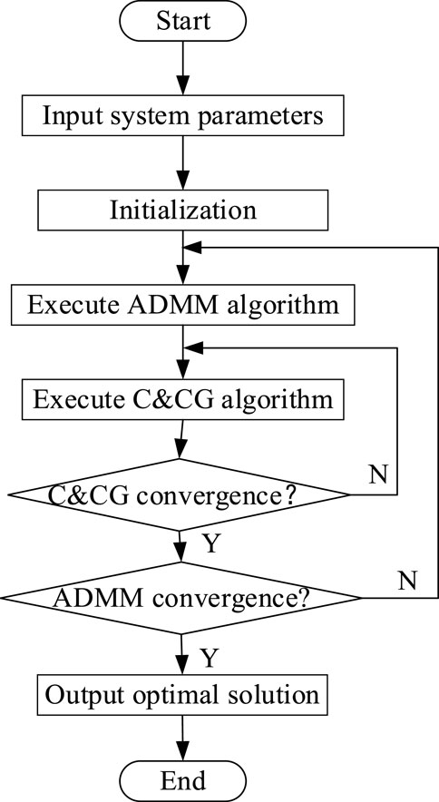
FIGURE 1. Overall flowchart of the proposed solving method.

5 Simulation example

5.1 Example parameters

The arithmetic model selected as a test example is shown in Figure 2. The upper-layer ESN includes a modified IEEE 33-node power system and a Belgian 20-node natural gas system, and the lower-layer DES model is a typical campus energy supply system. It should be pointed out that the method proposed in this study can be applied to different test examples, and only the relevant parameters need to be changed when applying to other test examples.

FIGURE 2

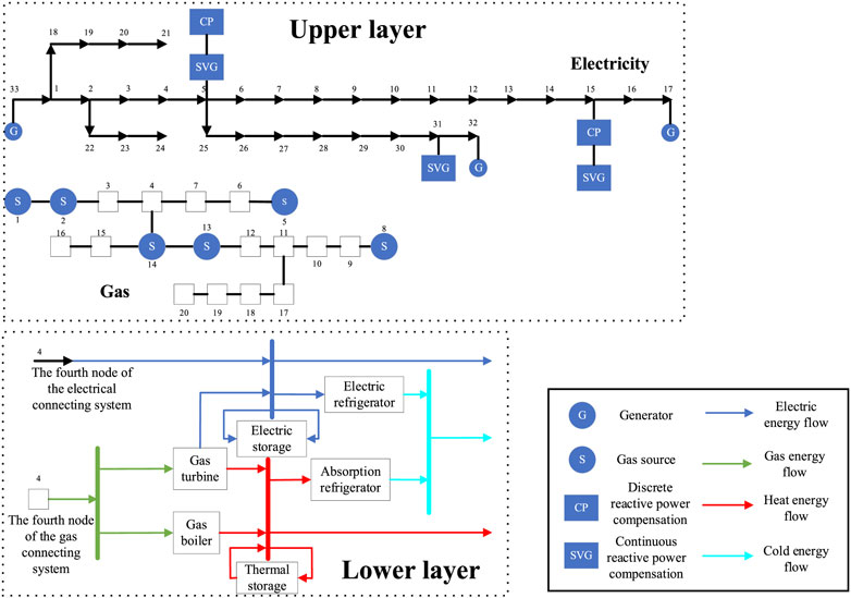
FIGURE 2. Model of the system used for simulation.

The forecast curves for each type of load in the lower-layer DES and PV are shown in Figure 3. Without loss of generality, the fluctuation range of the load is 0.1 of the predicted value, and the fluctuation range of PV is 0.15 of the predicted value. Figure 4 shows the time-of-use electricity price, and the gas price is set as 0.35 CNY/kW. The gas turbine’s maximum capacity is 1,400 kW, the maximum capacity of the gas boiler is 800 kW, the capacity of the electric chiller is 500 kW, the absorption chiller’s maximum capacity is 300 kW, the maximum storage capacity of electricity storage equipment and heat storage equipment is 1,500 kW h, and the minimum storage capacity is 200 kW h. The maximum value of charging and discharging power is 600 kW. Other parameters are selected according to references (Ding et al., 2017; Miao et al., 2020).

FIGURE 3

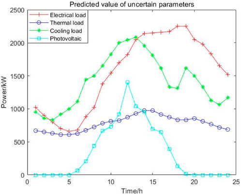
FIGURE 3. Predicted values of various loads and PV.

FIGURE 4

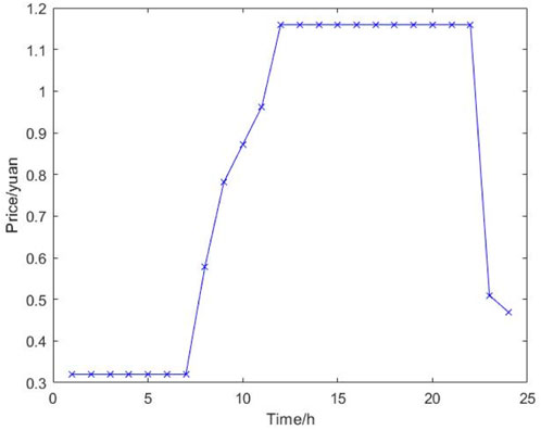
FIGURE 4. Time-of-use electricity price.

5.2 Simulation results

5.2.1 Convergence analysis

The convergence of ADMM and CCG algorithms is shown in Figure 5.

FIGURE 5

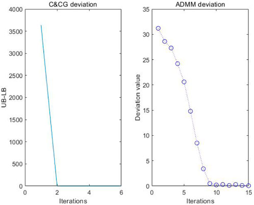
FIGURE 5. Convergence curves of the ADMM and CCG algorithms.

It can be seen from Figure 5 that both CCG and ADMM algorithms have fast convergence. The CCG algorithm almost converges to 0 after two iterations, while the ADMM algorithm needs nine iterations to obtain the optimal solution. This is because the initial value of the CCG algorithm is the predicted value of uncertain variables, and those predicted values are not very different from the final solution’s value. However, the initial value of the ADMM algorithm is set as 0, and the Lagrange coefficient increases with every iteration. At the same time, the difference between the upper and lower layers will become increasingly smaller to obtain the minimum (optimal) solution, which is the reason why the ADMM algorithm is slower than the CCG algorithm. It can be seen from the convergence diagram of the two algorithms that the ADMM algorithm is difficult to converge, which needs to be iterated nine times, while the CCG algorithm has already converged after two iterations. Therefore, the proposed method has high computational efficiency.

5.2.2 Voltage and air pressure analysis

The voltage and air pressure distribution diagrams of the upper-layer ESN are shown in Figures 6, 7, respectively.

FIGURE 6

FIGURE 6. Voltage distribution diagram.

FIGURE 7

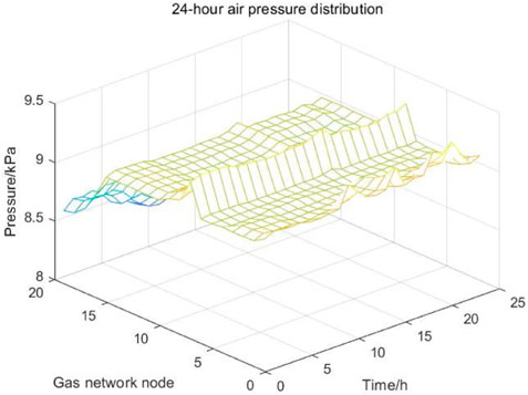
FIGURE 7. Gas pressure distribution diagram.

As shown in Figure 6, the voltage distribution of the power system of the RIES is between 0.94 and 1.06, which is within the permissible voltage limits and reflects the system’s high stability. The time and voltage magnitude relationship at node 1, for example, satisfies the load variations, with lower voltage magnitude during low-load layers and higher voltage magnitude during high-load layers. The voltage distribution corresponds to the generator access at the first hour. For example, the node closer to the generator has a higher voltage value, and the node with a higher distance from the generator has a lower voltage value.

Figure 7 shows that the air pressure distribution of the gas system of the RIES is between 8.5 and 9.5 kPa, which is in line with the engineering air pressure requirements. Therefore, the gas system has good stability. Similar to the voltage node, the barometric pressure value also corresponds to the gas source access node, i.e., the closer to the gas source node, the higher will be the barometric pressure value.

5.2.3 Equipment output analysis

The power balance diagrams of electricity, heat, and cooling of the lower-layer DES are shown in Figures 8, 9, 10, respectively.

FIGURE 8

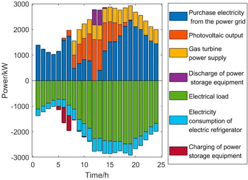
FIGURE 8. Electric-power balance.

FIGURE 9

FIGURE 9. Heat-power balance.

FIGURE 10

FIGURE 10. Cold-power balance.

Figure 8 presents the electrical load of the lower-layer DES which is mainly supplied by the purchased electricity. The gas turbine works at full load during the high-load period to reduce the pressure on the grid. Storage equipment charges during the low-load period and discharges during the high-load period to achieve peak shaving and valley filling of the electrical load, while discharging in time during the period when the electrical load just reaches its peak to avoid self-loss.

Figure 9 shows that the heat load mainly relies on the gas turbine, and the gas boiler is relied on only during the time when the gas turbine is out of service, which is because the gas turbine produces electricity and heat at the same time. Furthermore, charging and releasing the waste heat from electricity production can effectively reduce costs. Heat storage equipment is not operated because the heat load is small compared to other loads, and the peak-to-valley difference is not so evident. So, there is no high demand for heat storage, and at the same time, the process of charging, releasing, and storing heat will produce losses and increase the costs.

Figure 10 shows that the cooling load is mostly dependent on electric chillers to achieve the supply. This is due to the higher cooling factor of electric chillers, as electric chillers can directly convert electricity purchased from the grid to cooling energy, while heat is converted from gas and then converted again to cooling energy which will lead to higher losses.

5.2.4 Robustness analysis

Figures 11, 12 show the worst-case uncertainty parameters for the conservative adjustment parameters $\mathrm{\Gamma }=24$ and $\mathrm{\Gamma }=12$, respectively.

FIGURE 11

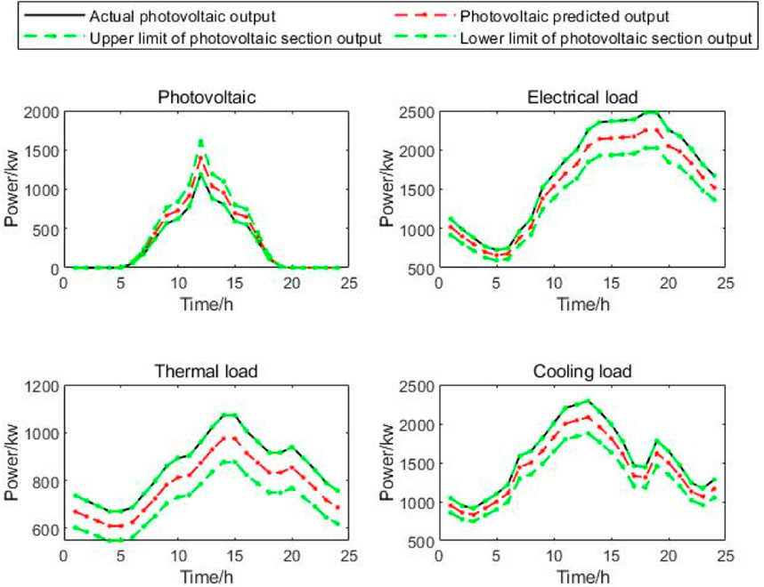
FIGURE 11. Uncertain parameters in the worst case for $\mathrm{\Gamma }=24$.

FIGURE 12

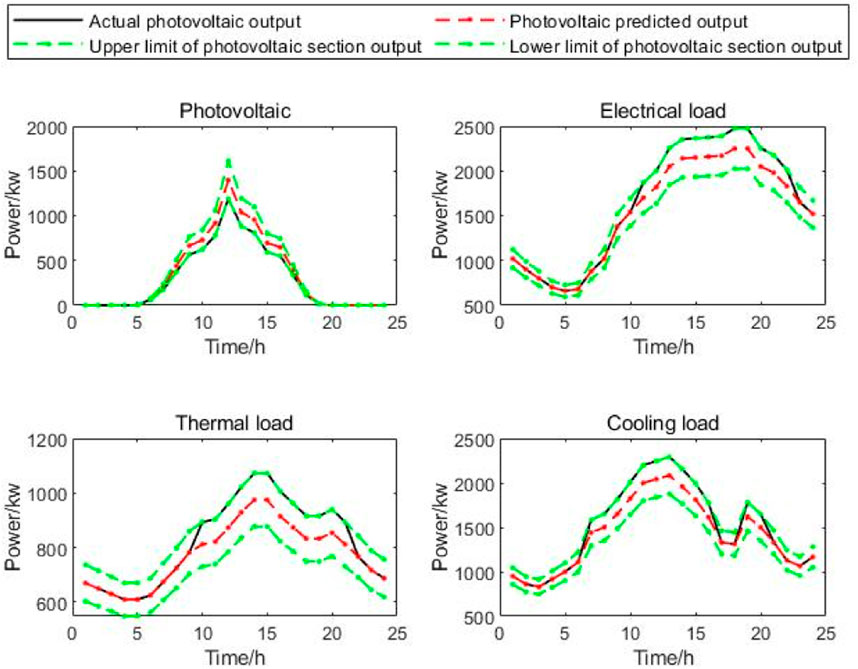
FIGURE 12. Uncertain parameters in the worst case for $\mathrm{\Gamma }=12$.

The sub-problem of the lower-layer DES is used to search for the worst-case scenario with uncertain parameters. Figures 11, 12 show that the worst-case scenarios are all those where the PV output is as small as possible and the load is as large as possible. For $\mathrm{\Gamma }=24$, the most conservative time occurs, where the worst-case scenario is that the PV output equals to the lower limit of the uncertainty interval, and the load equals the upper limit of the uncertainty interval in 24 h. For $\mathrm{\Gamma }=12$, the worst case for PV is reached only during 12 h because PV output is only in the daytime and the total output time is less than 12 h, so PV output is the minimum value in the uncertainty interval. For the load, the more output in the peak-energy consumption period, the greater the cost, so the worst case of load when its value reaches the maximum limit in the uncertainty interval appears only during 12 h, while the predicted value is maintained during the remaining hours.

In order to explore the influence of PV’s permeability on the results of this study, the following three scenarios are set. Scenario 1: all parameters are the same as the aforementioned example; scenario 2: the penetration level of PV is increased by 30%, and other parameters remain unchanged; and Scenario 3: the penetration level of PV is reduced by 30%, and the other parameters remain unchanged. Table 1 shows the simulation results of the scenarios obtained at $\mathrm{\Gamma }=0$, $\mathrm{\Gamma }=12$, and $\mathrm{\Gamma }=24$ when the worst-case scenario is applied. It can be seen that as the conservativeness parameter increases, the energy purchase cost gradually increases. Meanwhile, the supply deficit gradually decreases, which is due to the fact that the sub-problem of the lower-layer DES can search for the worst scenario and protect it in advance so that the supply deficit gradually decreases. However, this protection also comes at a cost, i.e., the energy purchase cost increases as well. The change in the conservativeness parameter from $\mathrm{\Gamma }=0$ to $\mathrm{\Gamma }=12$ increases the cost of energy purchase more and reduces the undersupply less than the change from $\mathrm{\Gamma }=12$ to $\mathrm{\Gamma }=24$. This is because the system prioritizes the protection of the worst scenarios (uncertain parameters at maximum load and maximum PV), followed by the protection of the less severe ones. Hence, the increase in the cost of energy purchase slows down with the increase in conservativeness, and the reduction in the undersupply slows down with the increase of conservativeness. It can be seen from Tables 1–3 that the penetration level of PV does not affect the aforementioned results. However, the greater the penetration level of PV, the lower the energy purchase cost of the system. Therefore, the greater the penetration level of PV in the system, the more robustly the system should be optimized.

TABLE 1

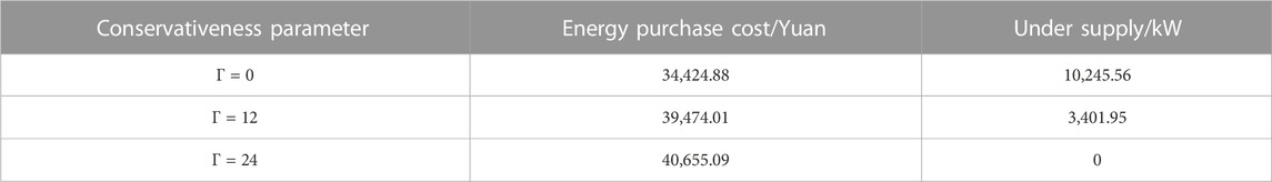
TABLE 1. Simulation results of scenario 1.

TABLE 2

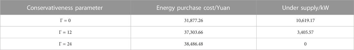
TABLE 2. Simulation results of scenario 2.

TABLE 3

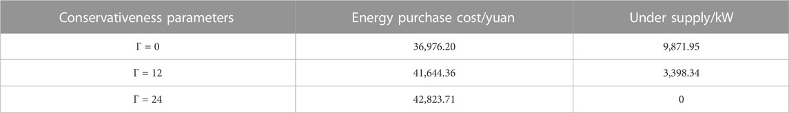
TABLE 3. Simulation results of scenario 3.

7 Conclusion

For reducing the negative impact of uncertainties brought by the DES on the system’s safe and reliable operation, a robust optimization model of the RIES considering uncertainties of the DES was developed in this study. First, the RIES with the DES was divided into an upper-layer ESN model and a lower-layer DES model according to their functions. The two layers were iteratively solved using the ADMM algorithm. Second, for the lower-layer DES, a two-stage robust optimization model was presented with the objective function of minimizing the energy purchase cost. In the first stage, the charging and discharging behaviors of storage equipment were explored, and in the second state, the optimal equipment output under the worst case could be developed. Then, for the sub-problem in the second stage, the bilinear terms were reduced to linear constraints using the big M method and solved using the CCG algorithm. Finally, the effectiveness of the proposed solving method was demonstrated by several simulation cases, which showed that the developed results could effectively suppress the uncertainty effects.

In future work, more focus will be given to the contradiction between the conservativeness of the robust optimization model and the optimization results. The robust optimization model based on the probability distribution function of uncertain variables can combine the possible probability distribution function of uncertain parameters to propose more targeted protection measures and reduce the conservativeness of the system. The robust optimization model based on the probability distribution function of uncertain variables will become an important direction for future research work. In addition, when considering larger-scale models and long-distance transmission models, losses should be taken into account, which are also the future research directions.

Data availability statement

The original contributions presented in the study are included in the article/Supplementary Material; further inquiries can be directed to the corresponding author.

Author contributions

XZ: methodology, software, writing—original draft, and data curation. YY: conceptualization of the study, supervision, and review and editing.

Funding

This work was supported by the National Natural Science Foundation of China (No. 51477041).

Conflict of interest

The authors declare that the research was conducted in the absence of any commercial or financial relationships that could be construed as a potential conflict of interest.

Publisher’s note

All claims expressed in this article are solely those of the authors and do not necessarily represent those of their affiliated organizations, or those of the publisher, the editors, and the reviewers. Any product that may be evaluated in this article, or claim that may be made by its manufacturer, is not guaranteed or endorsed by the publisher.

References

Balsamo, F., Falco, D. P., Mottola, F., and Pagano, M. (2020). Power flow approach for modeling shipboard power system in presence of energy storage and energy management systems. IEEE Trans. Energy Convers. 35, 1944–1953. doi:10.1109/tec.2020.2997307

CrossRef Full Text | Google Scholar

Ding, T., Li, C., Yang, Y., Jiang, J., Bie, Z., and Blaabjerg, F. (2017). A two-stage robust optimization for centralized-optimal dispatch of photovoltaic inverters in active distribution networks. IEEE Trans. Sustain. Energy 8, 744–754. doi:10.1109/tste.2016.2605926

CrossRef Full Text | Google Scholar

Ding, T., Liu, S., Yuan, W., Bie, Z., and Zeng, B. (2016). A two-stage robust reactive power optimization considering uncertain wind power integration in active distribution networks. IEEE Trans. Sustain. Energy 7, 301–311. doi:10.1109/tste.2015.2494587

CrossRef Full Text | Google Scholar

Farivar, M., and Low, S. H. (2013). Branch flow model: Relaxations and convexification—Part I. IEEE Trans. Power Syst. 28 (3), 2554–2564. doi:10.1109/TPWRS.2013.2255317

CrossRef Full Text | Google Scholar

Farivar, M., and Low, S. H. (2013). Branch flow model: Relaxations and convexification—Part II. IEEE Trans. Power Syst. 28 (3), 2565–2572. doi:10.1109/TPWRS.2013.2255318

CrossRef Full Text | Google Scholar

Feng, D., Lin, S., He, Z., Sun, X., and Wang, Z. (2018). Failure risk interval estimation of traction power supply equipment considering the impact of multiple factors. IEEE Trans. Transp. Electrification 4, 389–398. doi:10.1109/tte.2017.2784959

CrossRef Full Text | Google Scholar

Fu, Y., Lin, H., Ma, C., Sun, B., Li, H., Sun, Q., et al. (2021). Effects of uncertainties on the capacity and operation of an integrated energy system. Sustain. Energy Technol. Assessments 48, 101625. doi:10.1016/j.seta.2021.101625

CrossRef Full Text | Google Scholar

Li, J., Li, D., Zheng, Y., Yao, Y., and Tang, Y. (2022). Unified modeling of regionally integrated energy system and application to optimization. Int. J. Electr. Power & Energy Syst. 134, 107377. doi:10.1016/j.ijepes.2021.107377

CrossRef Full Text | Google Scholar

Li, P., Li, S., Yu, H., Yan, J., Ji, H., Wu, J., et al. (2022). Quantized event-driven simulation for integrated energy systems with hybrid continuous-discrete dynamics. Appl. Energy 307, 118268. doi:10.1016/j.apenergy.2021.118268

CrossRef Full Text | Google Scholar

Li, Q., Wang, S., Zhou, X., Zhang, A., and Zaman, R. (2021). Modeling and optimization of RIES based on composite energy pipeline energy supply. IEEE Trans. Appl. Supercond. 31, 1–5. doi:10.1109/tasc.2021.3090340

CrossRef Full Text | Google Scholar

Li, Y., Liu, C., Zhang, L., and Sun, B. (2021). A partition optimization design method for a regional integrated energy system based on a clustering algorithm. Energy 219, 119562. doi:10.1016/j.energy.2020.119562

CrossRef Full Text | Google Scholar

Li, Y., Wang, B., Yang, Z., Li, J., and Li, G. (2022). Optimal scheduling of integrated demand response-enabled community-integrated energy systems in uncertain environments. IEEE Trans. Industry Appl. 58, 2640–2651. doi:10.1109/TIA.2021.3106573

CrossRef Full Text | Google Scholar

Miao, B., Lin, J., Li, H., Liu, C., Li, B., Zhu, X., et al. (2020). Day-ahead energy trading strategy of regional integrated energy system considering energy cascade utilization. IEEE Access 8, 138021–138035. doi:10.1109/access.2020.3007224

CrossRef Full Text | Google Scholar

Rezaei, N., Pezhmani, Y., and Khazali, A. (2022). Economic-environmental risk-averse optimal heat and power energy management of a grid-connected multi microgrid system considering demand response and bidding strategy. Energy 240, 122844. doi:10.1016/j.energy.2021.122844

CrossRef Full Text | Google Scholar

Sioshansi, R., Denholm, P., Arteaga, J., Awara, S., Bhattacharjee, S., Botterud, A., et al. (2021). Energy-storage modeling: State-of-the-art and future research directions. IEEE Trans. Power Syst. 37, 860–875. doi:10.1109/tpwrs.2021.3104768

CrossRef Full Text | Google Scholar

Sun, T., Jiang, H., Cheng, L., and Zhu, W. (2018). Iteratively linearized reweighted alternating direction method of multipliers for a class of nonconvex problems. IEEE Trans. Signal Process. 66, 5380–5391. doi:10.1109/tsp.2018.2868269

CrossRef Full Text | Google Scholar

Wang, C., Yan, C., Li, G., Liu, S., and Bie, Z. (2020). Risk assessment of integrated electricity and heat system with independent energy operators based on Stackelberg game. Energy 198, 117349. doi:10.1016/j.energy.2020.117349

CrossRef Full Text | Google Scholar

Wang, Y., Huang, F., Tao, S., Ma, Y., Ma, Y., Liu, L., et al. (2022). Multi-objective planning of regional integrated energy system aiming at exergy efficiency and economy. Appl. Energy 306, 118120. doi:10.1016/j.apenergy.2021.118120

CrossRef Full Text | Google Scholar

Wang, Y., Zhao, S., Zhou, Z., Botterud, A., Xu, Y., and Chen, R. (2017). Risk adjustable day-ahead unit commitment with wind power based on chance constrained goal programming. IEEE Trans. Sustain. Energy 8, 530–541. doi:10.1109/tste.2016.2608841

CrossRef Full Text | Google Scholar

Xiang, Y., Cai, H., Liu, J., and Zhang, X. (2021). Techno-economic design of energy systems for airport electrification: A hydrogen-solar-storage integrated microgrid solution. Appl. Energy 283, 116374. doi:10.1016/j.apenergy.2020.116374

CrossRef Full Text | Google Scholar

Xu, X., Hu, S., Shi, P., Shao, H., Li, R., and Li, Z. (2022). Natural phase space reconstruction-based broad learning system for short-term wind speed prediction: Case studies of an offshore wind farm. Energy 2023, 125342. doi:10.1016/j.energy.2022.125342

CrossRef Full Text | Google Scholar

Yang, H., Liang, R., Yuan, Y., Chen, B., Xiang, S., Liu, J., et al. (2022). Distributionally robust optimal dispatch in the power system with high penetration of wind power based on net load fluctuation data. Appl. Energy 313, 118813. doi:10.1016/j.apenergy.2022.118813

CrossRef Full Text | Google Scholar

Zeng, B., and Zhao, L. (2013). Solving two-stage robust optimization problems using a column-and-constraint generation method. Operations Res. Lett. 41, 457–461. doi:10.1016/j.orl.2013.05.003

CrossRef Full Text | Google Scholar

Zhang, F., Wang, Y., Huang, D., Lu, N., Jiang, M., Wang, Q., et al. (2022). Integrated energy system region model with renewable energy and optimal control method. Front. Energy Res. 10, 1067202. doi:10.3389/fenrg.2022.1067202

CrossRef Full Text | Google Scholar

Zhang, J., Zhu, X., Chen, T., Yu, Y., and Xue, W. (2020). Improved MOEA/D approach to many-objective day-ahead scheduling with consideration of adjustable outputs of renewable units and load reduction in active distribution networks. Energy 210, 118524. doi:10.1016/j.energy.2020.118524

CrossRef Full Text | Google Scholar

Zhao, H., Wang, B., Pan, Z., Sun, H., Guo, Q., and Xue, Y. (2022). Aggregating additional flexibility from quick-start devices for multi-energy virtual power plants. IEEE Trans. Sustain. Energy 12, 646–658. doi:10.1109/tste.2020.3014959

CrossRef Full Text | Google Scholar

Zhao, Z., Wang, Y., Jiang, M., and Liu, X. (2022). Research on reliability assessment and multi-time scale improvement strategy of electricity-gas integrated energy system under cyber attack. Front. Energy Res. 10, 1049920. doi:10.3389/fenrg.2022.1049920

CrossRef Full Text | Google Scholar

Zhou, Y., and Zhang, J. (2020). Three-layer day-ahead scheduling for active distribution network by considering multiple stakeholders. Energy 207, 118263. doi:10.1016/j.energy.2020.118263

CrossRef Full Text | Google Scholar

Zhu, J., Mo, X., Xia, Y., Guo, Y., Chen, J., and Liu, M. (2022). Fully-decentralized optimal power flow of multi-area power systems based on parallel dual dynamic programming. IEEE Trans. Power Syst. 37, 927–941. doi:10.1109/tpwrs.2021.3098812

CrossRef Full Text | Google Scholar

Nomenclature

Parameters

$R_{ij}$, $X_{ij}$ Resistance/reactance of line $ij$

$n\left(j\right)$ Set of the sending nodes with node $j$ as the end node

$m\left(j\right)$ Set of the end nodes with node $j$ as the sending node

$\mathrm{\gamma }$ Maximum number of steps that can be adjusted

${\theta }_{\max }$ Maximum number of adjustments per day

$Q_{\mathrm{S}\mathrm{V}\mathrm{G}}^{\min }$, $Q_{\mathrm{S}\mathrm{V}\mathrm{G}}^{\max }$ Lower/upper limits of the regulation range

$\varsigma$ Efficiency factor of the pipe $q$

$T_0$ Standard temperature

$D_q$ Inner diameter of the pipe $q$

$p_0$ Standard pressure

$G$ Gas relative density

$L_q$ Length of the pipe $q$

$T_{qa}$ Average temperature of the pipe $q$

$Z_{qa}$ Average compression factor of the pipe $q$

$G_u$ Coefficient related to temperature and efficiency

$Z_u$ Other compression factor

$a$, $b$, $c$ Generators’ cost coefficients

$h$ Cost coefficient of gas supply

$N$, $M$ Total number of generators and gas sources

${\mathrm{\Theta }}^{\min }$, ${\mathrm{\Theta }}^{\max }$ Lower/upper limits of the variable ${\mathrm{\Theta }}^t$

${\eta }_{\mathrm{G}\mathrm{B}}$ Heat production efficiency

${\eta }_{\mathrm{G}\mathrm{T}}$ Power production efficiency

$\lambda$ Electricity-to-heat ratio

$CO{P}_{\mathrm{E}\mathrm{C}}$ Performance coefficient of the electric chiller

$CO{P}_{\mathrm{A}\mathrm{C}}$ Performance coefficient of the absorption chiller

$CO{P}_{\mathrm{A}\mathrm{C}}^0$ Rated conversion efficiency of the absorption chiller

$a_{\mathrm{A}\mathrm{C}}$, $b_{\mathrm{A}\mathrm{C}}$, $c_{\mathrm{A}\mathrm{C}}$ Conversion factors of the absorption chiller

${\beta }_{\mathrm{A}\mathrm{C}}$ Workload rate of the absorption chiller

${\delta }_i$ Self-loss rate of the energy storage device

${\eta }_{i,char}$, ${\eta }_{i,dis}$ Charging and discharging efficiencies of the energy storage device

$\mathrm{\Gamma }$, ${\mathrm{\Gamma }}_{pv}$, ${\mathrm{\Gamma }}_{i,\mathrm{L}}$ Uncertainty conservativeness adjustment parameters

$M_{BIG}$ Large positive real number, which is taken as 10⁹ in this study

$\epsilon$ Iteration convergence threshold of the CCG algorithm

Variables

$P_{jl}^t$, $Q_{jl}^t$ Active/reactive powers flowing from node $j$ to node $l$ at time $t$

$I_{ij}^t$ Current flowing through line $ij$ at time $t$

$U_i^t$ Voltage of node $i$ at time $t$

$Q_{\mathrm{C}\mathrm{P}}^t$ Compensated reactive power of the CP at time $t$

$Q_{\mathrm{C}\mathrm{P},\mathrm{U}}$ Reactive power output corresponding to each step of the CP

${\theta }_{\mathrm{C}\mathrm{P},m}^t$, ${\theta }_{\mathrm{C}\mathrm{P}\_\mathrm{a}\mathrm{d}\mathrm{d}}^t$, ${\theta }_{\mathrm{C}\mathrm{P}\_\mathrm{d}\mathrm{e}\mathrm{l}}^t$ A 0–1 variable

$Q_{\mathrm{S}\mathrm{V}\mathrm{G}}^t$ Reactive power of the SVG at time $t$

$P_{\mathrm{L},j}^t$, $Q_{\mathrm{L},j}^t$ Active/reactive loads of node $j$ at time $t$

$P_{\mathrm{G},j}^t$, $Q_{\mathrm{G},j}^t$ Active/reactive powers of the generator of node $j$ at time $t$

$f_q^t$ Flow of the pipe $q$ at time $t$

$p_m^t$ Pressure of node $m$ at time $t$

${\sigma }_u^t$ Gas flow consumed by the compressor $u$ at time $t$

${\alpha }_u$, ${\beta }_u$, ${\gamma }_u$ Energy consumption coefficients of the compressor $u$

$P_{\mathrm{c}\mathrm{o}\mathrm{m}}^t$ Gas energy consumed by the compressor $u$ at time $t$

$f_{com,u}$ Flow through compressor $u$ at time $t$

$f$ Branch flow vector

$\tau$ Compressor consumption flow vector

$A$ Branch node association matrix

$\varpi$ Node gas injection flow vector

$U$ Unit node association matrix

$T$ Compressor node association matrix

$G_G^t$ Gas supply quantity of the gas source at time $t$

$pric{e}_e^t$, $pric{e}_g^t$ Purchase prices of electricity and gas of the lower-layer DES at time $t$

$P_{grid}^t$, $P_{gas}^t$ Purchased power and gas power of the lower-layer DES from the upper-layer ESN at time $t$

$P_{G,k}^t$, $G_{G,k}^t$ The k-th generator and air source supply

${\mathrm{\Theta }}^t$ Other variables such as equipment output, voltage value, gas flow value, and node pressure

$H_{\mathrm{G}\mathrm{B}}^t$, $G_{\mathrm{G}\mathrm{B}}^t$ Heat production and gas consumption of the gas boiler at time $t$

$P_{\mathrm{G}\mathrm{T}}^t$ Power production of the gas turbine at time $t$

$G_{\mathrm{G}\mathrm{T}}^t$ Gas consumption of the gas turbine at time $t$

$H_{\mathrm{G}\mathrm{T}}^t$ Heat production of the gas turbine at time $t$

$C_{\mathrm{E}\mathrm{C}}^t$, $P_{\mathrm{E}\mathrm{C}}^t$ Cooling production and power consumption of the electric chiller at time $t$

$C_{\mathrm{A}\mathrm{C}}^t$, $H_{\mathrm{A}\mathrm{C}}^t$ Cooling production and heat consumption of the absorption chiller at time $t$

$E_i^t$ Reserves of energy storage at time $t$

$C_i^t$, $D_i^t$ Charging and discharging powers of the energy storage device

${\upsilon }_i$, $B_{i,\mathrm{L}}^t$, $D_{i,\mathrm{L}}^t$, $B_{\mathrm{P}\mathrm{V}}^t$, $D_{\mathrm{P}\mathrm{V}}^t$ 0–1 variables

$U$ Uncertainty set

$u_{\mathrm{P}\mathrm{V}}^t$, $u_{i,\mathrm{L}}^t$ Uncertainty variables of PV output and load power at time $t$ after introducing uncertainty

${\widehat{u}}_{\mathrm{P}\mathrm{V}}^t$, ${\widehat{u}}_{i,\mathrm{L}}^t$ Expected values of PV output and load power at time $t$

$\Delta u_{\mathrm{P}\mathrm{V}}^{\max ,t}$, $\Delta u_{i,\mathrm{L}}^{\max ,t}$ Maximum allowable deviations of PV output and load power at time $t$

$D_e^t$, $C_e^t$, $D_h^t$, $C_h^t$ Variables of charging and discharging powers corresponding to electric or thermal energies

$u_{e,\mathrm{L}}^t$, $u_{h,\mathrm{L}}^t$, $u_{c,\mathrm{L}}^t$ Variables of load uncertainty corresponding to electricity, heat, and cooling

${\omega }_1$, ${\omega }_2$, ${\omega }_3$ Dual variables in the lower-layer model

$B^{\prime }$ Auxiliary variable in the lower-layer model

$L_{up}$, $L_{dn}$ Augmented Lagrange function of the upper and lower layers

$P_{grid}^t$, $G_{gas}^t$ Global variables of purchased electricity and gas

$P_{grid,up}^t$, $G_{gas,up}^t$, $P_{grid,dn}^t$, $G_{gas,dn}^t$ Local variables of purchased electricity and gas in the upper and lower layers

$\eta$ Coefficient of the penalty term

${\lambda }_{1,up}^t$, ${\lambda }_{2,up}^t$, ${\lambda }_{1,dn}^t$, ${\lambda }_{2,dn}^t$ Lagrange multipliers

$\phi$ Maximum deviation of the ADMM algorithm