Multi-time-scale economic scheduling method for electro-hydrogen integrated energy system based on day-ahead long-time-scale and intra-day MPC hierarchical rolling optimization

To build a clean, secure, and efficient energy system, the hydrogen energy is an important developing trend for the energy revolution, and electro-hydrogen coupling system is expected to play an important role in the future. To obtain the optimal economic scheduling of the electro-hydrogen integrated energy system (E-H IES), this paper firstly establishes a refined model of the electrolyzer and hydrogen fuel cell and then proposes an optimal scheduling model based on day-ahead long-time-scale optimization and intra-day model predictive control (MPC) hierarchical rolling optimization. In the day-ahead stage, a long-time-scale optimization considering the impact of multi-day forecast information is proposed when performing the day-ahead optimization to achieve the effect of inter-day energy transfer of hydrogen energy and improve the overall economic efficiency. In addition, during the intra-day stage, the MPC is adopted to implement hierarchical rolling optimization to track and correct the day-ahead schedule and achieve coordinated operation between multi-energy systems while taking into account the different energy transfer characteristics. Finally, the simulation results demonstrate the feasibility of the proposed optimal scheduling model and the effectiveness of the proposed multi-time scale economic scheduling method.

1 Introduction

Environmental pollution and energy shortages lead to the urgent development of new energy sources. As a widely available, clean and efficient secondary energy source, hydrogen energy is an important carrier to support the transformation of energy and build a modern energy system (Huang et al., 2022). With the increasing penetration of renewable energy sources, the development of electro-hydrogen coupling will help to build a new type of power system (Pan et al., 2021; Pei et al., 2022). The optimal scheduling of the electro-hydrogen integrated energy system (E-H IES) will be an attractive problem which is vitally important to maximize its advantages.

At present, the optimal scheduling of the E-H IES mainly focuses on the following aspects, e.g., profit maximization (Taljan et al., 2008; El-Taweel et al., 2019; Tao et al., 2021), flexibility enhancement (Teng et al., 2019; Ma et al., 2022; Cheng et al., 2023), renewable energy consumption (Khalilnejad et al., 2018; Zhang and Yu, 2022), power fluctuations minimization (Chen et al., 2020; Wen et al., 2020). In (El-Taweel et al., 2019), a model of a private hydrogen storage station is proposed to maximize the benefits by changing the selling price of hydrogen. In (Ma et al., 2022), a Laplacian matrix is proposed to evaluate the effect of hydrogen vehicles on system flexibility improvement. Zhang and Yu (2022) proposes a dynamic programming algorithm to analyze the value of hydrogen energy in reducing carbon emissions and maximize the utilization of renewable energy. Chen et al. (2020) takes into account the challenges posed by the integration of large amounts of renewable energy into the grid, using hydrogen energy conversion to minimize power fluctuations. In the above literatures, the proposed problems are solved by adopting genetic algorithm, robust optimization, mixed integer linear programming and hybrid algorithm based on 24 h scheduling period. However, the above studies mostly ignore the effective utilization of hydrogen energy. In the electro-hydrogen coupling system, it is important to make full use of hydrogen energy storage systems (HESSs) characteristics to achieve the optimal distribution of energy on a long-time-scale. In general, electrical energy storage systems (EESSs) have short storage time and limited capacity scale. Currently, they are mainly used for regulating power grid frequency and peak, smoothing the fluctuation of renewable energy output, and implementing hourly short-cycle response and regulation. HESSs have the advantages of large storage capacity and long storage time, etc., which can be used in scenarios where electrochemical energy storage is insufficient. The existing research works rarely distinguish the storage characteristics of EESSs and HESSs which hinder the use of their respective strengths.

The coexistence and development of EESSs and HESSs are expected to play an important role in supporting the development of a large proportion of renewable energy (Gils et al., 2021). HESS is the optimal method for large-scale, long-term storage of centralized renewable energy due to its high energy density as an energy source (Yamamoto et al., 2021). Regarding the long-term storage of hydrogen energy, there are also some research works which are all manifested as seasonal storage of hydrogen energy (Converse, 2012; Li et al., 2020; Pan et al., 2020; Zhang et al., 2020). (Converse, 2012) is based on the combination of current data and social development to infer that the development of seasonal hydrogen storage is a wise choice in the future. Li et al. (2020), Zhang et al. (2020) carry out simulation analysis by giving case data and obtain the feasibility of seasonal storage through simulation results. Specifically (Zhang et al., 2020), gives the output data of wind turbine (WT) and photovoltaic (PV) for 8,760 h a year and conducts modeling analysis for 365 days a year (Pan et al., 2020). selects four typical days to represent the wind power and photovoltaic output of a year in spring, summer, autumn and winter.

Despite the fact that the aforementioned works have discussed the potential of hydrogen energy for long-term storage, there are still significant obstacles: 1) By using four typical days to represent the four seasons of the year, it is hard to truly reflect the storage situation of hydrogen energy in a year which makes it difficult to accurately simulate and exploit the advantages of seasonal storage of hydrogen energy. 2) If the data is given for 8,760 h a year, although it is possible to retain more comprehensive information on the timing of the various types of source loads, the sheer volume of data increases the complexity of the calculation and makes it difficult to solve. 3) It is true that inter-seasonal storage of hydrogen can solve the problem of uneven spatial and temporal distribution of renewable energy sources, but the above literature does not consider the security issues associated with the storage of large quantities of hydrogen, the volume of hydrogen storage tanks, the size of the capacity of electrolysis tanks and the spatial and temporal transport of hydrogen. All these issues are critical constraints for the inter-seasonal storage of hydrogen energy and need to be properly addressed.

Taking into account the fact that EESSs are difficult to conveniently store energy for long periods of time, and hydrogen energy, as a new energy source with its high energy density, can be the optimal solution for long-term energy storage. Therefore, this paper proposes an optimal operation framework for the electro-hydrogen coupled system considering multi-day forecast information. By considering the impact of future multi-day forecast information conditions on the current optimization when performing day-ahead optimization operations, the HESSs consider future renewable energy information and decide whether to transfer energy, thereby achieving optimal coordination between EESSs and HESSs. The optimized operation framework proposed in this paper has the following advantages: 1) By considering multi-day forecasting information, day-ahead optimized operation will produce hydrogen for storage when renewable energy is abundant and transfer this energy to be released when renewable energy is scarce. The overall economic efficiency of the system will be significantly improved, with a significant reduction in WT and PV abandonment. 2) It can implement the inter-day energy transfer of hydrogen energy, flexibly realize the two-way interactive transformation of electric energy-hydrogen energy and form a multi-energy complementary system to meet the diversified energy needs of electricity, heat and hydrogen according to local conditions. 3) The electric energy storage systems conduct intra-day energy transfer and the hydrogen storage systems perform inter-day energy transfer, which alleviates the excessive usage of electric energy storage to a certain extent and mitigates the loss of electric energy storage.

On the basis of the preceding study, we suggest a long-term day-ahead optimization that incorporates multi-day forecast information, i.e., the impact of future multi-day forecast information on the day-ahead optimization is also taken into account when executing the day-ahead optimization. A hierarchical rolling optimization is performed within the day using model predictive control (MPC) to track and correct the day-ahead schedule, taking into account the uncertainty of renewable energy sources and loads as well as the changes in the nature of different energy transfers. The main contributions of this paper are as follows.

1) A framework for optimizing the day-ahead long-time-scale operation of E-H IES considering multi-day forecast information is proposed, achieving the effect of inter-day energy transfer of hydrogen energy and intra-day energy transfer of electric energy, realizing that all energy that can be sold to the grid is sold and unsold energy is stored for hydrogen production, greatly reducing WT and PV abandonment and improving the economy of the system.

2) On the basis of the day-ahead optimized operation, the difference of different energy transmission properties of electricity-heat-hydrogen is considered. The MPC is used in the intra-day stage for tiered rolling control, which makes the scheduling arrangement more realistic.

3) Considering the intrinsic operating characteristics of electrolyzer and hydrogen fuel cell (HFC), proposing a refined model of electrolyzer and HFC, and considering the waste heat utilization link to realize the efficient utilization of energy.

The rest of the paper is organized as follows. Section 2 presents the structural model of the EH-IES. Section 3 presents the optimization framework. Section 4 introduces the optimization model and problem formulation. Section 5 and Section 6 are the case study and conclusion presentation, respectively.

2 The structural model of E-H IES

Figure 1 shows the structure of the E-H IES, which includes the energy supply side, the energy conversion side, the energy storage side, and the load side. Energy conversion is carried out through electro-hydrogen coupling to meet the needs of different energy sources of electricity-hydrogen-heat.

FIGURE 1

FIGURE 1. The structure of E-H IES.

2.1 Electrolyzer model

Regarding the electrolytic cells, there are mainly alkaline electrolytic cells, proton exchange membranes and solid oxide electrolytic cells. Alkaline electrolyzers are the most mature and widely used model, so this paper uses alkaline electrolyzers as an example. The waste heat generated by the electrolyzer is recycled, and the refined model of the hydrogen-heat cogeneration of the electrolyzer is proposed. Figure 2 shows the structure diagram of the refined utilization of the electrolytic cell. Electrolytic hydrogen production includes green electrolysis link, red heat transfer link and purple hydrogen energy utilization link.

FIGURE 2

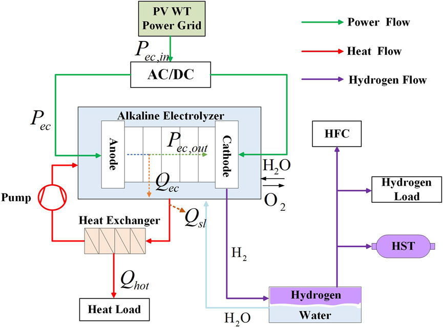
FIGURE 2. Diagram of refined utilization of electrolyzer.

Electrolysis link: During electrolysis, electrical energy is converted into hydrogen and heat. The relationship between the alternating current input to the electrolytic bath, the actual direct current used, and the hydrogen energy produced, and the heat energy is shown in (1–3).

$P_{ec,t}={\eta }_{ec}{P}_{ec,in,t}=U_{ec}\left(i_{ec,t},T_{ec,t}\right)i_{ec,t}=P_{ec,out,t}+Q_{ec,t}(1)$

$P_{ec,out,t}=i_{ec,t}{U}_{tn}\left(T_{ec,t}\right)={\eta }_{h_2}{P}_{ec,t}(2)$

$Q_{ec,t}=i_{ec,t}\left[U_{ec}\left(i_{ec,t},T_{ec,t}\right)-U_{tn}\left(T_{ec,t}\right)\right]={\eta }_h{P}_{ec,t}(3)$

where P_ec,t and P_ec,in,t are the input DC power and AC power to the electrolyzer; η_ec is electrolyzer AC/DC conversion efficiency; i_ec,t is current of the electrolyzer; T_ec,t is temperature of the electrolyzer; U_ec(i_ec,t, T_ec,t) is voltage function of electrolyzer; U_tn(T_ec,t) is thermoneutral voltage function of the electrolyzer; P_ec,out,t and Q_ec,t are hydrogen and heat production power of the electrolyzer; ${\eta }_{h_2}$ and η_h are hydrogen production efficiency and heat production efficiency of the electrolyzer.

In (2, 3), a non-linear relationship can be obtained between the thermal energy generated by the electrolyzer and the hydrogen energy and the temperature of the electrolyzer.

$Q_{ec,t}=\frac{P_{ec,out,t}}{U_{tn}\left(T_{ec,t}\right)}\left[U_{ec}\left(\frac{P_{ec,out,t}}{U_{tn}\left(T_{ec,t}\right)},T_{ec}\right)-U_{tn}\left(T_{ec,t}\right)\right](4)$

Due to the non-linear nature, it cannot be directly used in the optimal operation of E-H IES. The final model of the electrolysis link is obtained by linearizing it based on (Li et al., 2019; Pan et al., 2020).

$P_{ec,out,t}={\mu }_1{P}_{ec,in,t}+{\nu }_1{\delta }_{ec,t}{T}_{ec,t}(5)$

$Q_{ec,t}={\mu }_2{P}_{ec,in,t}+{\nu }_2{T}_{ec,t}(6)$

where μ₁, μ₂, ν₁, ν₂ denote the linearized parameters for the hot hydrogen co-production operating area of the electrolyzer; δ_ec,t is operating status of electrolyzer.

Heat transfer link: Some of the heat generated by the electrolyzer is lost and most of the rest goes to the heat exchanger. The heat entering the heat exchanger can either feed the heat load or optionally flow to the electrolyzer itself, maintaining the temperature of the electrolyzer itself. The electrolyzer can also choose to supply heat to the thermal load. The relationship between the final thermal energy supplied to the heat load and the thermal energy entering the heat exchanger is shown in (7). Quasi-steady state model of the electrolyzer temperature is expressed in (8). The thermal power lost by the electrolytic bath is shown by (9).

$Q_{he,t}={\eta }_{he}{Q}_{he,in,t}(7)$

$T_{ec,t+\mathrm{\Delta }t}=T_{ec,t}+\frac{\mathrm{\Delta }t}{C_{ec}}\left(Q_{ec,t}-Q_{sl,t}-Q_{he,in,t}\right)(8)$

$Q_{sl,t}=\left(T_{ec,t}-T_{\mathit{out,t}}\right)/R_{ec}(9)$

where Q_he,t is heat energy supplied to the heat load by the electrolyzer; η_he is conversion efficiency of heat energy in heat exchanger; Q_he,in,t is hermal energy of electrolyzer entering heat exchanger; Q_sl,t is thermal energy lost in the electrolyzer; C_ec is lumped heat capacity of electrolyzer; T_out,t is outdoor temperature; R_ec is lumped thermal resistance of electrolyzer. If Q_ec,t − Q_sl,t = Q_he,in,t, almost all of the waste heat is supplied to the heat load and the temperature of the electrolyzer is basically unchanged. If Q_ec,t − Q_sl,t > Q_he,in,t, some of the waste heat flows to the electrolyzer and the temperature of the electrolyzer rises. If Q_ec,t − Q_sl,t < Q_he,in,t, the electrolyzer releases some heat to the heat load and the corresponding temperature of the electrolyzer decreases.

In addition, the operation of the electrolyzer also needs to meet the start-stop constraints and operational constraints.

$\sum _{t=k}^{k+M_{ec,on,\min }-1}{\alpha }_{ec,on,t}\le 1(10)$

$\sum _{t=k}^{k+M_{ec,on,\min }-1}\left({\alpha }_{ec,on,t}+{\alpha }_{ec,off,t}\right)\le 1(11)$

$\sum _{t=k}^{k+M_{ec,off,\min }-1}{\alpha }_{ec,off,t}\le 1(12)$

$\sum _{t=k}^{k+M_{ec,off,\min }-1}\left({\alpha }_{ec,on,t}+{\alpha }_{ec,off,t}\right)\le 1(13)$

${\alpha }_{ec,on,t}+{\alpha }_{ec,off,t}\le 1(14)$

${\alpha }_{ec,on,t}-{\alpha }_{ec,off,t}={\delta }_{ec,t}-{\delta }_{ec,t-1}(15)$

$\sum _{t=1}^T{\alpha }_{ec,on,t}\le {\alpha }_{ec,on,\max }(16)$

$\sum _{t=1}^T{\alpha }_{ec,off,t}\le {\alpha }_{ec,off,\max }(17)$

${\delta }_{ec,0}={\delta }_{ec,T}(18)$

${\zeta }_{ec,\min }{\delta }_{ec,t}{C}_{\mathit{apa}}\le P_{ec,in,t}\le {\zeta }_{ec,\max }{\delta }_{ec,t}{C}_{\mathit{apa}}(19)$

$\left|P_{ec,in,t}-P_{ec,in,t-1}\right|\le \mathrm{\Delta }{P}_{ec,\max }(20)$

$T_{ec,\min }\le T_{ec,t}\le T_{ec,\max }(21)$

where M_ec,on, min and M_{ec,off, min} denote minimum operating time and minimum downtime for electrolyze; α_ec,on,t and α_ec,off,t denote 0–1 variables for electrolyzer start-up and shutdown actions; α_ec,on, max and α_{ec,off, max} denote the upper limit of the daily start and stop actions of the electrolyzer; ζ_ec, min and ζ_ec, max are minimum/maximum load rate of the electrolyzer; C_apa is electrolyzer capacity; ΔP_ec, max is the maximum ramping power of the electrolyzer; T_ec, min and T_ec, max are the minimum and maximum temperature of the electrolyzer. (10–13) limit the minimum working time and minimum downtime of the electrolyzer. (14) shows that the start-up and shutdown of an electrolytic cell cannot take place concurrently. (15) expresses the relationship between the state of the electrolytic cell switch and the start/stop action. (16) and (17) limit the number of start-ups and shutdowns of an electrolyzer per day. (18) ensures that the state of the electrolyzer before work is consistent with the state after work. (19) represents the relationship between the input electric power and the capacity of the electrolyzer. (20) and (21) represent the climbing constraints and the upper and lower temperature constraints for electrolyzer, respectively.

2.2 HFC model

The HFC supplies the electrical energy generated by the converter to the electrical load, and recycles the thermal energy generated by the stack reaction. The heat exchanger heats the return water of the circulating thermal system to supply the heat load and can also supply the fuel cell stack itself. HFC itself can absorb and release thermal energy. The relationship diagram of HFC cogeneration can be drawn, as shown in Figure 3. There is a clear proportional relationship between the electrical and thermal power generated by HFC. Considering that the loss of heat energy taken away by air flow does not affect the electrical output, the operating interval is shifted down overall from the ideal case. In the operating interval where air flow is considered, the highest electricity production efficiency is 0.6, corresponding to a heat production efficiency of 0.35, and the highest heat production efficiency is 0.53, corresponding to an electricity production efficiency of 0.33. According to the combined heat and power operating range of HFC, the operating model of the external characteristics of HFC can be summarized.

$P_{\mathit{hfc,t}}={\eta }_{\mathit{hfc,e,t}}{P}_{\mathit{hfc,in,t}}(22)$

$Q_{\mathit{hfc,t}}={\eta }_{\mathit{hfc,h,t}}{P}_{\mathit{hfc,in,t}}(23)$

${\eta }_{\mathit{hfc,e,min}}\le {\eta }_{\mathit{hfc,e,t}}\le {\eta }_{\mathit{hfc,e,max}}(24)$

${\eta }_{\mathit{hfc,h,min}}\le {\eta }_{\mathit{hfc,h,t}}\le {\eta }_{\mathit{hfc,h,max}}(25)$

${\eta }_{\mathit{hfc,h,t}}\le k_{h,\max }{\eta }_{\mathit{hfc,e,t}}(26)$

${\eta }_{\mathit{hfc,h,t}}\ge k_{e,\max }{\eta }_{\mathit{hfc,e,t}}(27)$

$Q_{\mathit{hfc,sl,t}}=\left(T_{\mathit{hfc,t}}-T_{\mathit{out,t}}\right)/R_{\mathit{hfc,ec}}(28)$

$P_{\mathit{hfc,in,t}}=P_{\mathit{hfc,t}}+Q_{\mathit{hfc,t}}+Q_{\mathit{hfc,sl,t}}(29)$

$Q_{\mathit{hfc,he,t}}={\eta }_{he}{Q}_{\mathit{hfc,he,in,t}}(30)$

$T_{\mathit{hfc,t+\Delta t}}=T_{\mathit{hfc,t}}+\frac{\mathrm{\Delta }t}{C_{\mathit{hfcc}}}\left(Q_{\mathit{hfc,t}}-Q_{\mathit{hfc,he,in,t}}\right)(31)$

${\zeta }_{\mathit{hfc,min}}{\delta }_{\mathit{hfc,t}}{C}_{\mathit{apb}}\le P_{\mathit{hfc,in,t}}\le {\zeta }_{\mathit{hfc,max}}{\delta }_{\mathit{hfc,t}}{C}_{\mathit{apb}}(32)$

$\left|P_{\mathit{hfc,in,t}}-P_{\mathit{hfc,in,t-1}}\right|\le \mathrm{\Delta }{P}_{\mathit{hfc,max}}(33)$

$T_{\mathit{hfc,min}}\le T_{\mathit{hfc,t}}\le T_{\mathit{hfc,max}}(34)$

where P_hfc,t and Q_hfc,t denote electricity and thermal energy generated by HFC; P_hfc,in,t is hydrogen power input HFC; η_hfc,e,t and η_hfc,h,t denote electricity generation efficiency and heat generation efficiency of HFC; η_hfc,e,min and η_hfc,e,max are minimum and maximum efficiency of electricity generation; η_hfc,h,min and η_hfc,h,max are minimum and maximum efficiency of heat generation; k_h, max and k_e, max are the slope of maximum thermal efficiency and electrical efficiency operating boundary; Q_hfc,sl,t is the heat energy lost by HFC; T_hfc,t is the temperature of the HFC; R_hfc,ec is lumped thermal resistance of HFC; Q_hfc,he,t is the heat energy supplied by HFC to the heat load; Q_hfc,he,in,t is the heat energy entering the heat exchanger; η_he is the heat efficiency; C_hfcc is lumped heat capacity of HFC; δ_hfc,t is perating status of HFC; ζ_hfc,min and ζ_hfc,max are the minimum and maximum load rate of the HFC; C_apb is HFC Capacity; ΔP_hfc,max is the maximum ramping power of the HFC; T_hfc,min and T_hfc,max are the minimum and maximum temperature of HFC. (22) and (23) express the relationship between the power generation and heat generation and the input hydrogen energy. (24) and (25) place limits on the efficiency of heat production and electricity production respectively. (26) and (27) ensure that HFC operates within the allowable range. The thermal power lost by HFC is shown by (28). (29) ensures that the input and output energy of HFC is conserved. (30) represents the relationship between the thermal energy supplied to the heat load and the thermal energy entering the heat exchanger. Eq. 31 is a quasi-steady-state model of HFC temperature. (32) represents the relationship between the input hydrogen power and the capacity of HFC. (33) and (34) represent the climbing constraint and the upper and lower temperature constraints for HFC, respectively.

FIGURE 3

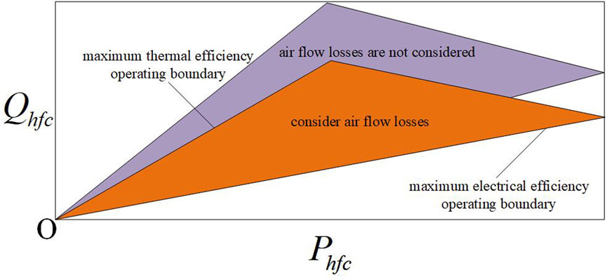
FIGURE 3. HFC cogeneration operating range.

There are non-linear terms in (22, 23) for the product of two continuous variables. To simplify the computation, the following linearized transformation of the non-linear terms is performed using the binary method and the big M method.

$W^x=W_{\min }^x+y\sum _{n=0}^p{2}^n{\delta }_n^x(35)$

$0\le y\sum _{n=0}^p{2}^n{\delta }_n^x\le W_{\max }^x-W_{\min }^x(36)$

${\delta }_n^x\in \left\{\mathrm{0,1}\right\}(37)$

$m{W}^x=m{W}_{\min }^x+y\sum _{n=0}^p{2}^n{\tau }_n^x(38)$

$m-M\left(1-{\delta }_n^x\right)\le {\tau }_n^x\le m+M\left(1-{\delta }_n^x\right)(39)$

$-M{\delta }_n^x\le {\tau }_n^x\le M{\delta }_n^x(40)$

where m and W^x are continuous variables. ${\delta }_n^x$ is a binary variable. ${\tau }_n^x$ is an auxiliary variable. M is a very large number. $W_{\max }^x$ and $W_{\min }^x$ are the maximum and minimum values of the continuous variable W^x, respectively. p is the number of digits in the binary. y is the resolution.

2.3 Hydrogen storage tank (HST) model

In this paper, the ideal gas equation of state is used to describe the relationship between the hydrogen mass and the pressure in HST.

$P_{\mathit{HST,t}}{V}_{\mathit{HST}}=n_{\mathit{HST,t}}R{T}_H(41)$

$n_{\mathit{HST,t}}=\frac{m_{\mathit{HST,t}}}{M_{H_2}}(42)$

$P_{\mathit{HST,min}}\le P_{\mathit{HST,t}}\le P_{\mathit{HST,max}}(43)$

$m_{\mathit{HST,t+1}}=m_{\mathit{HST,t}}+m_{\mathit{HST,in,t}}-m_{\mathit{HST,out,t}}(44)$

$0\le m_{\mathit{HST,in,t}}\le B_{\mathit{HST,in,t}}{m}_{\mathit{HST,in,max}}(45)$

$0\le m_{\mathit{HST,out,t}}\le B_{\mathit{HST,out,t}}{m}_{\mathit{HST,out,max}}(46)$

$B_{\mathit{HST,in,t}}+B_{\mathit{HST,out,t}}\le 1(47)$

where P_HST,t is the pressure of the HST; V_HST is the volume of the HST; n_HST,t is amount of hydrogen substance; R is ideal gas constant; T_H is gas temperature; m_HST,t is mass of hydrogen; $M_{H_2}$ is molar mass of hydrogen; P_HST,min and P_HST,max are the minimum and maximum pressure of HST; m_HST,in,t and m_HST,out,t are hydrogen storage and release in HST; m_HST,in,max and m_HST,out,max are the maximum hydrogen storage and release rate; B_HST,in,t and B_HST,out,t are HST hydrogen storage and release 0–1 variable. (43–47) shows the operating model of HST. (43) is the pressure safe operating range of HST. (44) is the relationship between the hydrogen mass in HST at two adjacent moments. (45, 46) are the maximum constraints of hydrogen storage and hydrogen release. (47) is the constraint of hydrogen storage state and hydrogen release state to ensure that the HST does not store and release hydrogen at the same time.

2.4 EESSs model

Electric energy storage model including energy model (48–53) and life model (54–58).

$E_t=E_{t-\mathrm{\Delta }t}-P_{\mathit{dis,t}}\mathrm{\Delta }t/{\eta }_d+{\eta }_c{P}_{ch,t}\mathrm{\Delta }t(48)$

$0\le P_{ch,t}\le B_{ch,t}{P}_{ch,\max }(49)$

$0\le P_{\mathit{dis,t}}\le B_{\mathit{dis,t}}{P}_{\mathit{dis,max}}(50)$

$B_{ch,t}+B_{\mathit{dis,t}}\le 1(51)$

$E_{\min }\le E_t\le E_{\max }(52)$

$E_0=E_T(53)$

${\mathrm{\Gamma }}_R=L_R{D}_R{C}_R(54)$

$d_{\mathit{eff}}=k_0\left(1-k_{1}SO{C}_t+k_{2}SO{C}_t^2\right)(55)$

$k_0=e^{u_1-1+\frac{1}{D_R}}{d}_R/D_R^{u_0}(56)$

$k_1=u_0+u_1/D_R(57)$

$k_2=u_0\left(u_0-1\right)/2+u_0{u}_1/D_R+u_1^2/2D_R^2(58)$

where E_t is the amount of electricity contained in the EES; P_ch,t and P_dis,t are charging and discharging power; η_c and η_d are charging and discharging efficiency; P_ch, max and P_dis,max are the maximum charging and discharging power; B_ch,t and B_dis,t are charging and discharging 0–1 flag variable; E_min and E_max are the minimum and maximum energy of EES; E₀ and E_T are the initilal and the end energy of EES; Γ_R represents the rated usage Ampere hours of the electric energy storage; L_R is the rated cycle life; d_R is rated Ampere hours consumed by single discharge; D_R is rated depth of discharge; C_R is rated ampere-hour capacity. d_eff represents the ampere-hours consumed by a single use of electrical energy storage; SOC is the state of charge of the EES; k₀, k₁, k₂ are constants. u₀, u₁ are the parameter values obtained from the test during the simulation process.

3 Optimization framework

This paper proposes a day-ahead long-time-scale optimization considering multi-day forecast information and an intra-day MPC hierarchical rolling optimization operation strategy. The proposed optimized operation framework is shown in Figure 4. The multi-time scale in this paper consists of two stages.

FIGURE 4

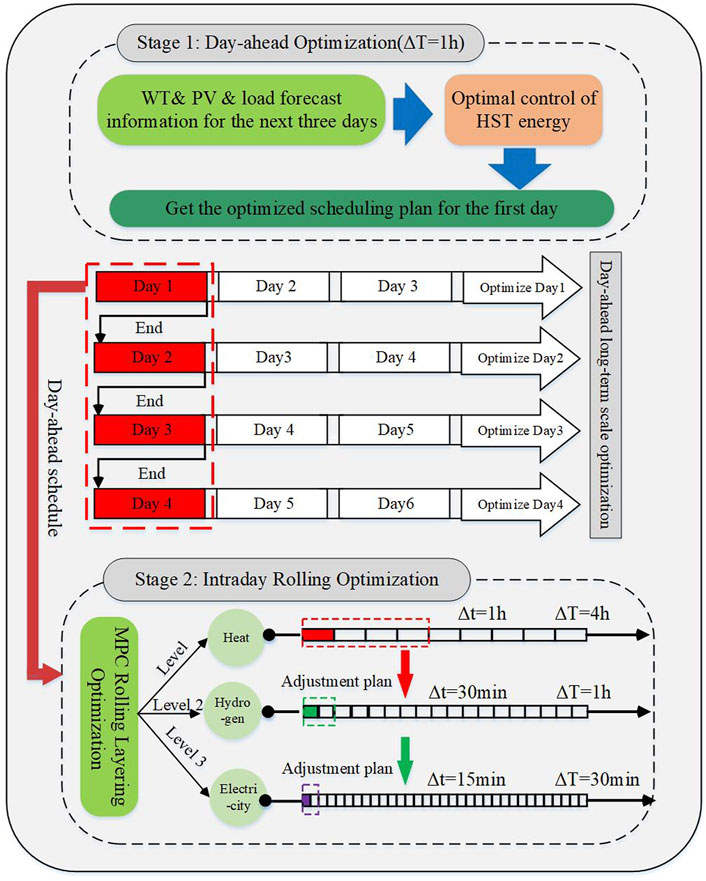
FIGURE 4. The proposed framework.

Stage 1: day-ahead optimization. When performing day-ahead optimization, the optimization duration is not 24 h on the short-time-scale. The system considers not only the WT, PV and load information of the day, but also the forecast information of the next few days. The system only retains the optimized operation results for the first day. After the first day’s optimization is complete, the system’s scheduling information is transferred to the second day, where the identical optimization approach is executed. In this way, the inter-day energy transfer of hydrogen energy is implemented in the day-ahead long-time-scale optimization considering multi-day forecast information.

Stage 2: intra-day rolling optimization. To solve the uncertainty of wt, pv and load day-ahead output, MPC is used for rolling optimization control during intra-day. Considering the difference among various energy transport properties of electricity-heat-hydrogen, this paper sets the control period for heat to 1 h and the prediction period to 4 h, the control period for hydrogen to 30 min and the prediction period to 1 h, and the control period for electricity to 15 min and the prediction period to 30 min. The day-ahead plan is tracked and corrected through the MPC rolling control.

4 Problem formulation

In the proposed E-H IES optimization operation strategy, the overall economic efficiency of the optimization cycle is optimized by taking forecast information for several days into account.

4.1 Day-ahead optimization

4.1.1 Objective function

A mixed-integer linear programming (MILP) problem is posed during day-ahead optimization. The objective function is to minimize the overall operating cost of the system.

$F=\min \left(f_1+f_2+f_3+f_4-f_5\right)(59)$

$f_1=\sum _{t=1}^T\left(c_{in,t}{P}_{in,t}-c_{\mathit{out,t}}{P}_{\mathit{out,t}}\right)(60)$

$f_2=\sum _{t=1}^T{K}_{in}{\lambda }_{in}{P}_{in,t}(61)$

$f_3=\sum _{t=1}^T\left(d_{\mathit{eff}}/{\mathrm{\Gamma }}_R\right)C_s(62)$

$f_4=\sum _{t=1}^T\left(\alpha \mathrm{\Delta }{P}_{pv,t}+\beta \mathrm{\Delta }{P}_{wt,t}\right)(63)$

$f_5=\sum _{t=1}^T\left(\rho Q_{yl,t}\right)(64)$

where c_in,t and c_out,t are the price of electricity purchase and sale; P_in,t and P_out,t are the electricity purchased and sold; K_in is conversion factor for converting electricity purchased into carbon; λ_in is environmental penalty factor for CO ₂ emissions; C_s is the investment cost of EES; α and β are penalty factor for abandoning WT and PV; ΔP_pv,t and ΔP_wt,t are abandoned PV and WT power; ρ is heat selling price; Q_yl,t is the heat energy sold by the system; (60) represents the transaction cost with the upper-level grid. (61) represents the system carbon emission cost. (62) represents the life loss cost of electrical energy storage. (63) represents the cost of abandoning WT and PV. (64) represents the profit from the sale of some heat energy.

4.1.2 Operation constraints

$P_{pv,t}+P_{wt,t}+P_{in,t}+P_{\mathit{dis,t}}+P_{\mathit{hfc,t}}=P_{ec,in,t}+P_{ch,t}+P_{\mathit{out,t}}+P_{gl,t}+P_{\mathit{load,t}}(65)$

$Q_{gl,t}+Q_{he,t}+Q_{\mathit{hfc,he,t}}+Q_{\mathit{dis,t}}=Q_{\mathit{heat,t}}+Q_{ch,t}+Q_{yl,t}(66)$

$P_{ec,out,t}+m_{\mathit{HST,out,t}}HH{V}_{h_2}=P_{h_2,t}+m_{\mathit{HST,in,t}}HH{V}_{h_2}+P_{\mathit{hfc,in,t}}(67)$

$0\le P_{in,t}\le F_{in,t}{P}_{in,\max }(68)$

$0\le P_{\mathit{out,t}}\le F_{\mathit{out,t}}{P}_{\mathit{out,max}}(69)$

$F_{in,t}+F_{\mathit{out,t}}\le 1(70)$

$Q_{gl,t}={\eta }_{gl}{P}_{gl,t}(71)$

$Q_{gl,\min }{U}_{gl,t}\le Q_{gl,t}\le Q_{gl,\max }{U}_{gl,t}(72)$

$\sum _{t=1}^T\left|U_{gl,t}-U_{gl,t-1}\right|\le N_{gl}(73)$

where P_pv,t and P_wt,t are PV and WT power; P_gl,t is the electric power generated by the electric boiler; P_load,t is load demand; Q_gl,t is the thermal energy generated by the electric boiler; Q_ch,t and Q_dis,t are the heat charging and releasing of the HST; Q_heat,t is heat load; $HH{V}_{h_2}$ is high calorific value of hydrogen; $P_{h_2,t}$ is hydrogen load; P_in, max and P_out,max are the maximum purchase and sale electricity; F_in,t and F_out,t are electricity purchase and sale 0–1 flag variable; η_gl is electric boiler electric heat conversion efficiency; Q_gl, min and Q_gl, max are the minimum and maximum heat output of electric boilers; U_gl,t is the start-stop state of the electric boiler; N_gl is daily maximum start and stop times of electric boiler. (65), (66), and (67) represent the electrical, thermal, and hydrogen power balances, respectively. (68–70) represents the constraint relationship between the system and the grid tie line. The operating constraints of electric boilers include (71–73).

4.2 Intra-day rolling optimization

Although the renewable energy forecasting technology is always evolving and the forecasting accuracy is constantly improving, the optimized operation results derived by considering only the day-ahead renewable energy and load output may differ from the actual operation results.

Model predictive control (MPC) has the characteristics of rolling optimization and feedback correction (Ye et al., 2022), which can update the state of the system in real time and reduce the system error caused by inaccurate prediction. MPC mainly includes three steps: model prediction, rolling optimization and feedback correction (Vasilj et al., 2019).

4.2.1 Model prediction

Model prediction is to predict the future output of the system based on historical information, and optimize the control to make the final output as close to the reference value as possible. Predictive models emphasize system inputs and outputs rather than the model’s specific structure. In this paper, the incremental state space model is used as the system control expression, as shown in (74).

$\left\{\begin{array}{c}\hfill \mathrm{\Delta }x\left(k+1\right)=A\mathrm{\Delta }x\left(k\right)+B\mathrm{\Delta }u\left(k\right)+D\mathrm{\Delta }e\left(k\right)\hfill \\ \hfill y\left(k\right)=C\mathrm{\Delta }x\left(k\right)+y\left(k-1\right)\hfill \end{array}\right.(74)$

where Δx(k), Δu(k), Δe(k), and y(k) represent the state variables, input variables, the increase of disturbance variables and output variables of the system, respectively. A, B, C, D are system control parameters.

According to (74), the predicted output of the system at time (k + j) can be written as follows,

$\begin{array}{cc}\hfill y\left(k+j|k\right)=& \sum _{i=0}^{j}C{A}^i\mathrm{\Delta }x\left(k\right)+\sum _{i=1}^{j}C{A}^{i-1}B\mathrm{\Delta }u\left(k\right)+\sum _{i=1}^{j}C{A}^{i-1}B\mathrm{\Delta }u\left(k+1\right)\hfill \\ \hfill & +\cdots +\sum _{i=1}^{j-m+1}C{A}^{i-1}B\mathrm{\Delta }u\left(k+m-1\right)\hfill \\ \hfill & +\sum _{i=1}^{j}C{A}^{i-1}D\mathrm{\Delta }e\left(k\right)+y\left(k\right)\hfill \end{array}(75)$

where j is the prediction period, and m is the control period.

4.2.2 Rolling optimization

MPC performs optimization solution by rolling forward, calculates the optimal control sequence according to the optimization index in the forecast period at each control moment, and continuously updates the forecast period. In general, the minimum weighted sum of the variance of the actual output and the reference trajectory and the variance of the control variable can be taken as the system optimization index, as shown below:

$minJ\left(k\right)=P\sum _{j=1}^M{‖y\left(k+j\right)-y\left(k+j|k\right)‖}^2+Q\sum _{j=1}^M{‖\mathrm{\Delta }u\left(k+j|k\right)‖}^2(76)$

where P and Q are the weighting matrices of the output and control variables, respectively. M is the prediction time domain.

4.2.3 Feedback correction

To ensure that the system state will not significantly deviate from the safe and normal range in the event of system error interference, the system only executes the control plan at the current timestep. In the next timestep, the system will re-predict, and then compensate for the latest error during the subsequent optimization procedures. The above process constitutes a closed-loop feedback system, which makes the system optimization control strategy more effective. The system updates the error through (77).

$\left\{\begin{array}{c}\hfill \mathrm{\Delta }r\left(k\right)=y\left(k\right)-y\left(k|k-1\right)\hfill \\ \hfill \mathrm{\Delta }x\left(k+1\right)=\mathrm{\Delta }x\left(k+1|k\right)+{\lambda }_r\mathrm{\Delta }r\left(k\right)\hfill \end{array}\right.(77)$

where, Δr(k) is the actual deviation between the predicted value and the actual value, and λ_r is the error coefficient matrix.

4.2.4 Hierarchical optimization

The E-H IES contains various types of energy such as electricity, hydrogen, and heat. Due to the various transmission properties of multiple energy sources, if the dynamic characteristics of various energy sources are ignored in the operation optimization of E-H IES, the final output plan will depart significantly from the real situation. Therefore, on the basis of MPC, this paper proposes a hierarchical optimization operation method that considers the difference of energy transmission characteristics.

The dynamic characteristics of various energy networks in E-H IES are highly distinct, and so is the response of each piece of equipment to the system. Among them, the power transmission speed and the response speed to the system power fluctuation are the quickest. It can be considered that the power transmission is completed instantaneously. In general, the transient process of the power transmission does not need to be considered in the scheduling. The hydrogen transmission may be affected by the pipeline, the transmission speed is relatively slow, and the influence of the transient process needs to be considered in the optimal scheduling. The transmission speed of thermal energy is the slowest of the three types of energy, as it transmits thermal energy through mediums such as hot water.

In the multi-time-scale optimization of E-H IES, the planned output of each piece of equipment in the next day is obtained through day-ahead optimization, and the scheduling period is 1 h. Intra-day hierarchical rolling optimization is an adjustment to the day-ahead plan. Among them, the intra-day control period of thermal energy is 1 h, and the prediction period is 4 h. The intra-day control period of hydrogen energy is 30 min, and the prediction period is 1 h. The intra-day control period of electric energy is 15 min, and the prediction period is 30 min.

Thermal energy control scheduling: This stage is to adjust the output of heat-generating equipment according to the day-ahead output plan and the deviation of predicted heat load. The objective is to minimize the operating cost of the thermal layer and the power adjustment cost of related components.

$\begin{array}{ll}\hfill F_{\mathit{heat}}=& \min \sum _{t=1}^{T_{\mathit{heat}}}\left(-\rho Q_{yl,t}+S_{gl}\left|\mathrm{\Delta }{Q}_{gl,t}\right|+S_{\mathit{TST}}\left|\mathrm{\Delta }{Q}_{\mathit{tst,t}}\right|+S_{ez}\left|\mathrm{\Delta }{Q}_{he,t}\right|\right.\hfill \\ \hfill & \left.+S_{\mathit{hfc}}\left|\mathrm{\Delta }{Q}_{\mathit{hfc,he,t}}\right|\right)\hfill \end{array}(78)$

where T_heat is heat intra-day scheduling cycle; S_gl is electric boiler unit power adjustment cost; S_TST is TST unit power adjustment cost; S_ez is electrolyzer unit power adjustment cost; S_hfc is HFC unit power adjustment cost; ΔQ_gl,t is difference between the heat production of electric boiler and the day-ahead plan; ΔQ_tst,t is difference between TST output and day-ahead plan; ΔQ_he,t is difference between heat production of the electrolyzer and day-ahead plan; ΔQ_hfc,he,t is difference between HFC heat production and day-ahead plan.

Hydrogen energy control scheduling: This stage is to adjust the output of hydrogen-generating equipment according to the output plan of the day-ahead and the output plan of the thermal layer and the deviation of the hydrogen load prediction. The objective is to minimize the operating cost of the hydrogen layer and the power adjustment cost of related components.

$\begin{array}{ll}\hfill F_{\mathit{hydrogen}}& =\min \sum _{t=1}^{T_{\mathit{hydrogen}}}\left(\alpha \mathrm{\Delta }{P}_{pv,t}+\beta \mathrm{\Delta }{P}_{wt,t}+S_{\mathit{HST}}\left|\mathrm{\Delta }{M}_{\mathit{hst,t}}\right|+S_{ez}\left|\mathrm{\Delta }{P}_{ec,out,t}\right|\right.\hfill \\ \hfill & \left.+S_{\mathit{hfc}}\left|\mathrm{\Delta }{P}_{\mathit{hfc,in,t}}\right|\right)\hfill \end{array}(79)$

where T_hydrogen is hydrogen intra-day scheduling cycle; S_HST is HST unit power adjustment cost; ΔM_hst,t is difference between HST output and day-ahead plan; ΔP_ec,out,t is difference between the hydrogen produced by electrolyzer and the plan of the thermal dispatch layer; ΔP_hfc,in,t is difference between the hydrogen consumption of HFC and the plan of the thermal dispatch layer.

Electric energy control scheduling: This stage is to adjust the output of power equipment according to the output plan of the day-ahead, the output plan of the thermal layer, the output plan of the hydrogen layer, the deviation of the electric load forecast and the deviation of the wind power photovoltaic prediction. The objective is to minimize the operating cost of the electrical layer and the power adjustment cost of related components.

$F_{\mathit{ele}}=\min \sum _{t=1}^{T_{\mathit{ele}}}\left\{\begin{array}{c}\hfill ci{n}_t{P}_{in,t}-cou{t}_t{P}_{\mathit{out,t}}+K_{in}{\lambda }_{in}{P}_{in,t}+\left(d_{\mathit{eff}}/{\mathrm{\Gamma }}_R\right)C_s+\alpha \mathrm{\Delta }{P}_{pv,t}+\beta \mathrm{\Delta }{P}_{wt,t}+\hfill \\ \hfill S_{gl}\left|\mathrm{\Delta }{P}_{gl,t}\right|+S_{\mathit{EES}}\left|\mathrm{\Delta }{E}_{\mathit{ees,t}}\right|+S_{ez}\left|\mathrm{\Delta }{P}_{ec,in,t}\right|+S_{\mathit{hfc}}\left|\mathrm{\Delta }{P}_{\mathit{hfc,t}}\right|+S_{\mathit{grid}}\left|\mathrm{\Delta }{P}_{\mathit{grid,t}}\right|\hfill \end{array}\right\}(80)$

where T_ele is electric intra-day scheduling cycle; S_EES is EES unit power adjustment cost; S_grid is grid contact lines unit power adjustment cost; ΔE_ees,t is difference between EES output and day-ahead plan; ΔP_ec,in,t is difference between the electric energy consumed by the electrolyzer and the plan of the hydrogen dispatch layer; ΔP_hfc,t is difference between the electric energy consumed by HFC and the plan of the hydrogen dispatch layer; ΔP_grid,t is difference between the power of the contact line and the day-ahead plan.

5 Case study

To validate the effectiveness of the proposed day-ahead scheduling strategy comparisons between the proposed strategy and traditional day-ahead optimization are illustrated. In the intra-day stage, MPC is used to track and correct the day-ahead plan obtained by the proposed approach.

5.1 System parameters and data

The structure diagram of the E-H IES is shown in Figure 1. Load, photovoltaic and wind power forecast information are shown in Figures 5, 6, respectively. The parameters of some devices are shown in Table 1.

FIGURE 5

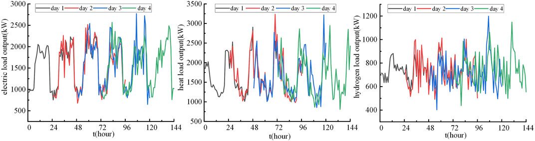
FIGURE 5. Electricity-heat-hydrogen load forecast information.

FIGURE 6

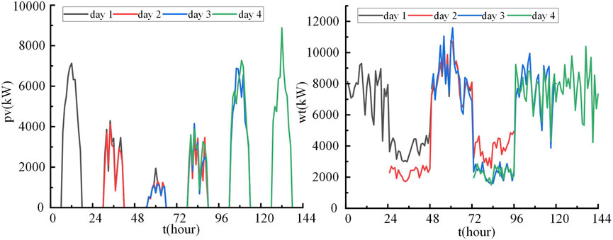
FIGURE 6. PV and WT forecast information.

TABLE 1

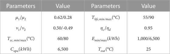
TABLE 1. Parameters of related devices.

The World Meteorological Organization divides weather forecasts into three categories based on their duration: very short-range weather forecasting (next 12 h), short-range weather forecasting (next 3 days) and medium-range weather forecasting (next 10 days). In order to consider both the long-term operation of hydrogen energy and the accuracy of the forecast, this paper chooses to predict the information of the next 3 days. In addition, renewable energy and load forecasting are not the focus of this paper.

5.2 Day-ahead optimization

The comparison cases in this paper are as follows.

Case 1: Traditional day-ahead optimization.

Case 2: Day-ahead optimization considering multi-day forecast information.

To see the transfer effect of hydrogen energy more intuitively, a 4-day optimization operation is conducted. In Case 1 and Case 2, the energy changes of electric and hydrogen energy storage are shown in Figure 7. The relationship between thermal energy and temperature in the electrolyzer and HFC is shown in Figures 8, 9, respectively.

FIGURE 7

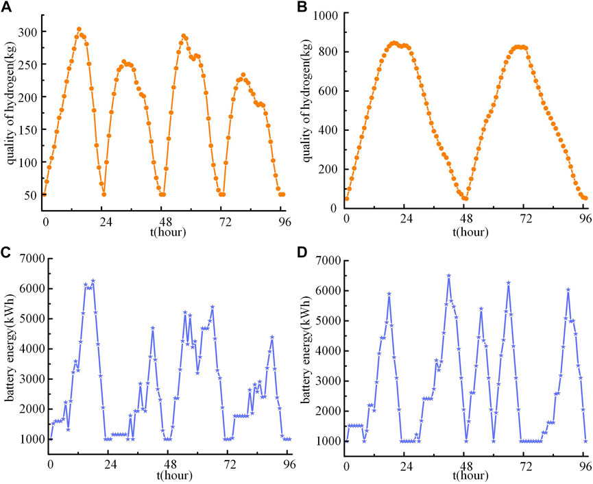
FIGURE 7. HES and EES energy. (A) Case 1 HES. (B) Case 2 HES. (C) Case 1 EES. (D) Case 2 EES.

FIGURE 8

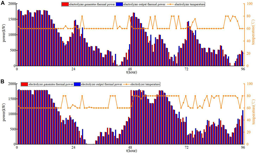
FIGURE 8. The relationship between thermal energy and temperature of electrolyzer. (A) Case 1. (B) Case 2.

FIGURE 9

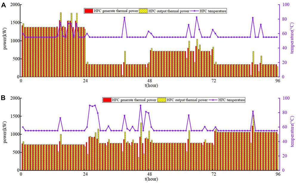
FIGURE 9. The relationship between thermal energy and temperature of HFC. (A) Case 1. (B) Case 2.

Figure 6 depicts the weather conditions over the next 4 days. The changes in the quality of hydrogen in the HST in cases 1 and case 2 are significant. In the traditional day-ahead optimization, the energy of hydrogen returns to its initial state at the end of each day, which can only meet the daily energy demand. In day-ahead optimization that considers multi-day forecast information, hydrogen is stored while renewable energy is abundant and released when it is scarce. The proposed method maximizes the use of renewable energy, resolves the problem of uneven distribution of renewable energy, and implement the inter-day energy transfer for hydrogen energy. Under the traditional optimal operation strategy, the electric energy storage is frequently charged and discharged and the SOC of electric energy storage is at a low level. The day-ahead optimal operation strategy proposed in this paper shows that the frequency of charging and discharging of electric energy storage is reduced and the SOC is at a high level, which has a certain mitigation effect on the life depreciation of electric energy storage. The proposed day-ahead long-time-scale optimal operation strategy achieves the inter-day energy transfer of hydrogen energy storage and the intra-day energy transfer of electric energy storage, and realizes the coordinated control of multiple types of energy storage.

Renewable energy is abundant in the system on the first and third days, when the electrolyzer produces a large amount of hydrogen with a large amount of heat. In case 1, the electrolyzer must continue to operate on the second and fourth days to maintain a balance between hydrogen energy and heat energy. However, in case 2, the HST plays a significant role on the second and fourth days, and the HFC can use this portion of the free resources to generate heat. In the day-ahead optimization considering multi-day forecast information, it is evident that the electrolyzer can reduce some workload when wind and solar resources are insufficient, thereby preventing damage to the equipment from excessive use. Based on the heat generation and the heat supply to the heat load, the temperature of the electrolyzer changes accordingly.

In case 1, on the first day when renewable energy is abundant, HFC employs hydrogen to generate a great deal of heat to prevent excessive abandonment of wind power and photovoltaics. When renewable energy is scarce, hydrogen is provided primarily to the hydrogen load, with any excess going to the HFC. Thus, the output of the HFC is relatively low. In case 2, when the renewable energy is sufficient, the HFC uses the hydrogen generated by the electrolyzer to work, as the HFC cannot work with the hydrogen stored in the HST, and the output of the HFC remains stable.

In the day-ahead stage, the power balances of different energy sources in case 1 and case 2 are shown in Figures 10, 11, respectively. In case 1, when the renewable energy is sufficient, E-H IES chooses to sell electricity to the upper power grid to make a profit. Under the penalty of abandoning wind power and photovoltaics, part of the renewable energy is converted into hydrogen through the electrolyzer, and HFC uses this part of the hydrogen to generate heat for sale. When there is a shortage of renewable energy, the system can only choose to buy electricity from the upper-level grid to meet the system demand, and the system does not sell heat to the outside. The traditional day-ahead optimization may obtain greater benefits in some cases, but in the long-term development, it is not a smart development model.

FIGURE 10

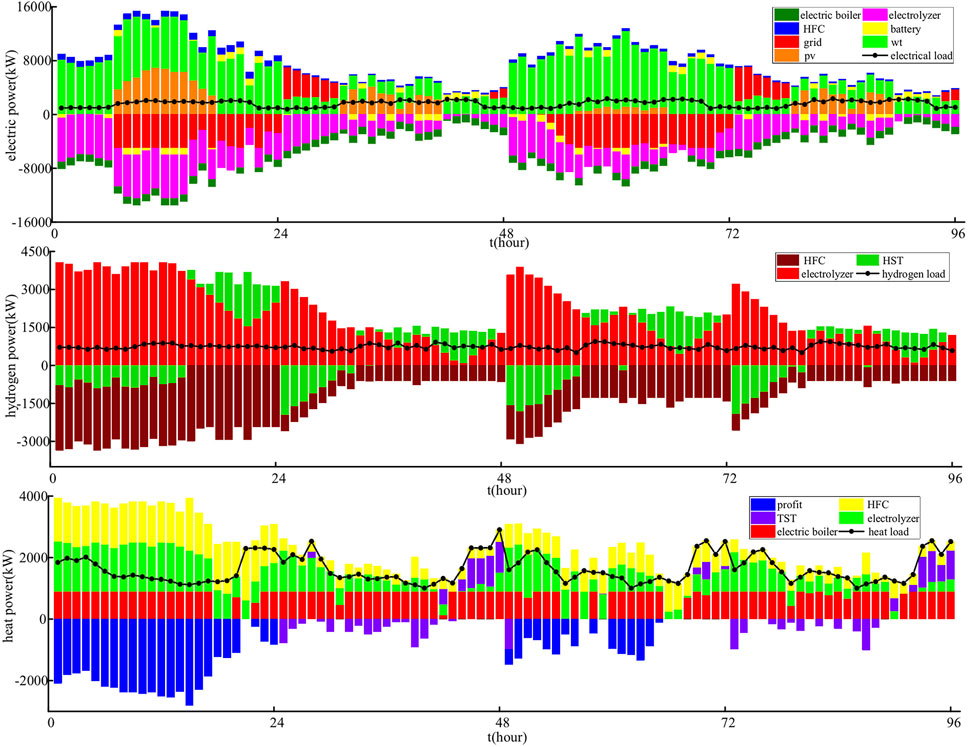
FIGURE 10. Power balance of different energy sources in case 1.

FIGURE 11

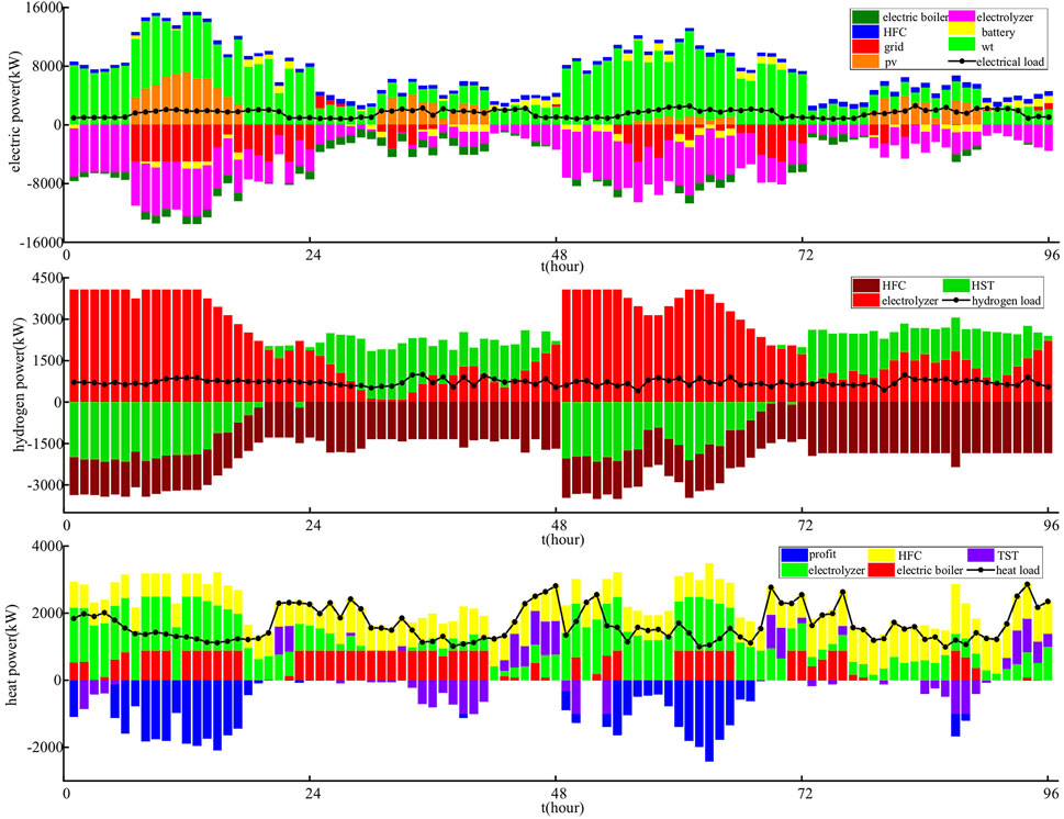
FIGURE 11. Power balance of different energy sources in case 2.

In case 2, from the electricity-hydrogen-thermal coupling point of view, the HST is almost in the storage state on the first and third days and is released for system usage on the second and fourth days. When renewable energy is in excess, the system also sells power and heat. When there is a shortage of renewable energy, the system not only greatly reduces the purchase of electricity from the upper grid, but also has a small profit from heat sales. The system’s overall economic value is then significantly enhanced.

Comparisons of case 1 and case 2 are shown in Table 2. It can be calculated from Table 2 that the average cost of case 1 is −24,435.8 yuan, while the average cost of case 2 is −32,421.7 yuan. The average life of the EES in case 1 is 5.80605 years, and the average life of the EES in case 2 is 6.1829 years. It can be seen that the profitability of case 1 is slightly higher than that of case 2 on the first and third days, but it is much lower than that of case 2 on the second and fourth days. From the perspective of long-term development of the system, day-ahead optimization considering multi-day forecast information can tackle the problem of uneven distribution of renewable energy. The overall economic effect of the system is better, and it also has a certain mitigation effect on the loss of EES, reducing the abandonment of wind power and photovoltaics in the system.

TABLE 2

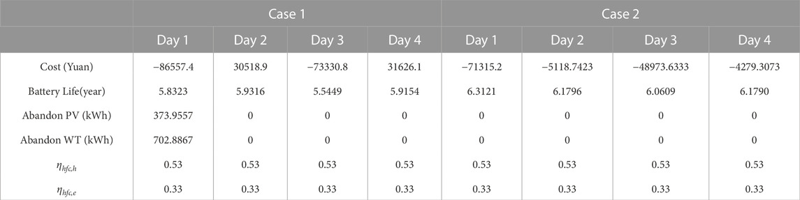
TABLE 2. Optimization results for two cases.

5.3 Intra-day rolling optimization

After the day-ahead plan is obtained, MPC is used to track and correct the day-ahead plan within the day. Since the steps of intra-day rolling are the same, this paper only analyses the intra-day optimization on the first day. According to the different dispatch periods of electricity-heat-hydrogen, Figure 12 shows the comparison results of the load day-ahead forecast and the intra-day forecast, respectively.

FIGURE 12

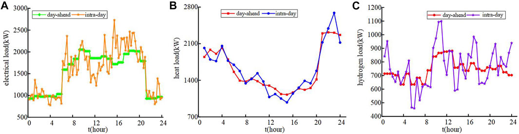
FIGURE 12. Intra-day forecast data. (A) Electricity load. (B) Heat load. (C) Hydrogen load.

In the heat energy dispatching stage, the output adjustment of related heat equipment and thermal storage tank (TST) is mainly determined by the heat load prediction inaccuracy. Since the heat energy dispatching cycle is the longest, as the first stage of intra-day dispatching, it is sufficient to follow the system’s day-ahead plan and analyze the system operating economy and the output fluctuation of each component under the premise of meeting the load requirements. In the second stage of intra-day hydrogen scheduling, in addition to following the system’s day-ahead output plan, it also needs to follow the adjustment plan of the thermal energy scheduling stage. In the hydrogen scheduling stage, the output adjustment of the relevant hydrogen energy equipment is mostly determined by the hydrogen load prediction inaccuracy. Electric energy dispatching has the shortest cycle and is also the last stage of intra-day dispatching. On the basis of following the system’s day-ahead output plan, it is also necessary to meet the output adjustment plans of each component in the first two stages. In the electric energy dispatching stage, the output adjustment of related electric energy equipment and EES is mainly carried out according to the electric load and the forecast error of wind power photovoltaic. Figure 13 shows intra-day heat balance, hydrogen balance, and electrical power balance, respectively.

FIGURE 13

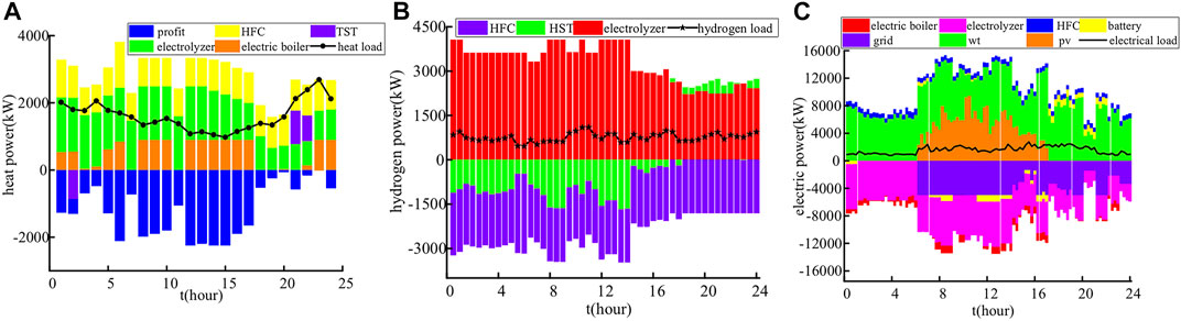
FIGURE 13. Intra-day operation. (A) Heat balance. (B) Hydrogen balance. (C) Electrical power balance.

6 Conclusion

This paper proposes a multi-time-scale optimization operation strategy, which includes day-ahead long-time-scale optimization considering multi-day forecast information and intra-day MPC hierarchical rolling optimization. In the day-ahead stage, the system achieves a balanced distribution of renewable energy via hydrogen energy transfer by incorporating forecast information for multi-day in the future. In the intra-day stage, using MPC to track and revise the day-ahead plan, more precise scheduling control is obtained with consideration of variable energy transmission qualities. The case analysis shows that.

1) Compared with the typical day-ahead optimization, the proposed day-ahead optimization that takes into account the multi-day forecast information enables the inter-day energy transfer of hydrogen energy, for sake that the electric energy storage has a greater impact on intra-day energy transfer. With the cooperation of the long-time-scale of hydrogen energy and the short-time-scale of electric energy, the overall economy of the system has been improved, the utilization rate of renewable energy has been greatly improved, and there is also a certain protective effect on the life of electric energy storage.

2) Since there are errors in the forecast of renewable energy and load, as well as differences in the transmission qualities of various energy sources, hierarchical rolling optimization through MPC is required to track and adjust the day-ahead plan, resulting in a more accurate dispatch plan.

Data availability statement

The original contributions presented in the study are included in the article/Supplementary Material, further inquiries can be directed to the corresponding author.

Author contributions

LZ: Conceptualization, methodology, validation, software, investigation, writing–review editing, project administration, resources. WD: Methodology, software, formal analysis, validation, writing–original draft, visualization, funding acquisition. BZ: Methodology, validation, writing–review editing, project administration. XZ: Methodology, validation, writing–review editing, project administration. ML: Methodology, validation, writing–review editing, project administration. QW: Methodology, validation, writing–review editing, project administration. JC: Methodology, writing–review editing, supervision.

Funding

This work was supported by Research on multi-time scale coordinated control and operation optimization technology of distributed electro-hydrogen coupling system, Science and Technology Project of State Grid Zhejiang Electric Power Co., Ltd. (No. B311DS221003).

Conflict of interest

LZ, BZ, XZ, ML, and QW were employed by State Grid Zhejiang Electric Power Research Institute.

The remaining authors declare that the research was conducted in the absence of any commercial or financial relationships that could be construed as a potential conflict of interest.

Publisher’s note

All claims expressed in this article are solely those of the authors and do not necessarily represent those of their affiliated organizations, or those of the publisher, the editors and the reviewers. Any product that may be evaluated in this article, or claim that may be made by its manufacturer, is not guaranteed or endorsed by the publisher.

References

Chen, X., Cao, W., Zhang, Q., Hu, S., and Zhang, J. (2020). Artificial intelligence-aided model predictive control for a grid-tied wind-hydrogen-fuel cell system. IEEE Access 8, 92418–92430. doi:10.1109/ACCESS.2020.2994577

CrossRef Full Text | Google Scholar

Cheng, L., Zang, H., Wei, Z., and Sun, G. (2023). Secure multi-party household load scheduling framework for real-time demand-side management. IEEE Trans. Sustain. Energy 14, 602–612. doi:10.1109/TSTE.2022.3221081

CrossRef Full Text | Google Scholar

Converse, A. O. (2012). Seasonal energy storage in a renewable energy system. Proc. IEEE 100, 401–409. doi:10.1109/JPROC.2011.2105231

CrossRef Full Text | Google Scholar

El-Taweel, N. A., Khani, H., and Farag, H. E. Z. (2019). Hydrogen storage optimal scheduling for fuel supply and capacity-based demand response program under dynamic hydrogen pricing. IEEE Trans. Smart Grid 10, 4531–4542. doi:10.1109/TSG.2018.2863247

CrossRef Full Text | Google Scholar

Gils, H. C., Gardian, H., and Schmugge, J. (2021). Interaction of hydrogen infrastructures with other sector coupling options towards a zero-emission energy system in Germany. Renew. Energy 180, 140–156. doi:10.1016/j.renene.2021.08.016

CrossRef Full Text | Google Scholar

Huang, J., Wu, X., Zheng, Z., Huang, Y., and Li, W. (2022). Multi-objective optimal operation of combined cascade reservoir and hydrogen system. IEEE Trans. Ind. Appl. 58, 2836–2847. doi:10.1109/tia.2021.3138949

CrossRef Full Text | Google Scholar

Khalilnejad, A., Sundararajan, A., and Sarwat, A. I. (2018). Optimal design of hybrid wind/photovoltaic electrolyzer for maximum hydrogen production using imperialist competitive algorithm. J. Mod. Power Syst. Clean. Energy 6, 40–49. doi:10.1007/s40565-017-0293-0

CrossRef Full Text | Google Scholar

Li, J., Lin, J., Song, Y., Xing, X., and Fu, C. (2019). Operation optimization of power to hydrogen and heat (p2hh) in adn coordinated with the district heating network. IEEE Trans. Sustain. Energy 10, 1672–1683. doi:10.1109/TSTE.2018.2868827

CrossRef Full Text | Google Scholar

Li, J., Lin, J., Zhang, H., Song, Y., Chen, G., Ding, L., et al. (2020). Optimal investment of electrolyzers and seasonal storages in hydrogen supply chains incorporated with renewable electric networks. IEEE Trans. Sustain. Energy 11, 1773–1784. doi:10.1109/TSTE.2019.2940604

CrossRef Full Text | Google Scholar

Ma, X., Zhou, H., and Li, Z. (2022). Toward the resilient design of interdependencies between hydrogen refueling and power systems. IEEE Trans. Ind. Appl. 58, 2792–2802. doi:10.1109/TIA.2021.3122401

CrossRef Full Text | Google Scholar

Pan, G., Gu, W., Lu, Y., Qiu, H., Lu, S., and Yao, S. (2020). Optimal planning for electricity-hydrogen integrated energy system considering power to hydrogen and heat and seasonal storage. IEEE Trans. Sustain. Energy 11, 2662–2676. doi:10.1109/TSTE.2020.2970078

CrossRef Full Text | Google Scholar

Pan, G., Hu, Q., Gu, W., Ding, S., Qiu, H., and Lu, Y. (2021). Assessment of plum rain’s impact on power system emissions in yangtze-huaihe river basin of China. Nat. Commun. 12, 6156. doi:10.1038/s41467-021-26358-w

PubMed Abstract | CrossRef Full Text | Google Scholar

Pei, W., Zhang, X., Deng, W., Tang, C., and Yao, L. (2022). Review of operational control strategy for dc microgrids with electric-hydrogen hybrid storage systems. CSEE J. Power Energy Syst. 8, 329–346. doi:10.17775/CSEEJPES.2021.06960

CrossRef Full Text | Google Scholar

Taljan, G., Canizares, C., Fowler, M., and Verbic, G. (2008). The feasibility of hydrogen storage for mixed wind-nuclear power plants. IEEE Trans. Power Syst. 23, 1507–1518. doi:10.1109/TPWRS.2008.922579

CrossRef Full Text | Google Scholar

Tao, Y., Qiu, J., Lai, S., and Zhao, J. (2021). Integrated electricity and hydrogen energy sharing in coupled energy systems. IEEE Trans. Smart Grid 12, 1149–1162. doi:10.1109/TSG.2020.3023716

CrossRef Full Text | Google Scholar

Teng, Y., Wang, Z., Li, Y., Ma, Q., Hui, Q., and Li, S. (2019). Multi-energy storage system model based on electricity heat and hydrogen coordinated optimization for power grid flexibility. CSEE J. Power Energy Syst. 5, 266–274. doi:10.17775/CSEEJPES.2019.00190

CrossRef Full Text | Google Scholar

Vasilj, J., Gros, S., Jakus, D., and Zanon, M. (2019). Day-ahead scheduling and real-time economic mpc of chp unit in microgrid with smart buildings. IEEE Trans. Smart Grid 10, 1992–2001. doi:10.1109/TSG.2017.2785500

CrossRef Full Text | Google Scholar

Wen, T., Zhang, Z., Lin, X., Li, Z., Chen, C., and Wang, Z. (2020). Research on modeling and the operation strategy of a hydrogen-battery hybrid energy storage system for flexible wind farm grid-connection. IEEE Access 8, 79347–79356. doi:10.1109/ACCESS.2020.2990581

CrossRef Full Text | Google Scholar

Yamamoto, H., Fujioka, H., and Okano, K. (2021). Cost analysis of stable electric and hydrogen energy supplies derived from 100% variable renewable resources systems. Renew. Energy 178, 1165–1173. doi:10.1016/j.renene.2021.06.061

CrossRef Full Text | Google Scholar

Ye, Q., Lin, H., Jin, J., and Chen, W. (2022). An optimal dispatching strategy of island microgrid considering economy and flexibility. Zhejiang Electr. Power 41, 54–64. doi:10.19585/j.zjdl.202203007

CrossRef Full Text | Google Scholar

Zhang, Y., and Yu, Y. (2022). Carbon value assessment of hydrogen energy connected to the power grid. IEEE Trans. Ind. Appl. 58, 2803–2811. doi:10.1109/TIA.2021.3126691

CrossRef Full Text | Google Scholar

Zhang, M., Zhang, N., Guan, D., Ye, P., Song, K., Pan, X., et al. (2020). Optimal design and operation of regional multi-energy systems with high renewable penetration considering reliability constraints. IEEE Access 8, 205307–205315. doi:10.1109/ACCESS.2020.3036640

CrossRef Full Text | Google Scholar