An effective approach for deriving and evaluating approximate optimal design solutions of energy supply systems by time series aggregation

It is important to design multi-energy supply systems optimally in consideration of their operations for variations in energy demands. An approach for efficiently solving such an optimal design problem with a large number of periods for variations in energy demands is to derive an approximate optimal design solution by time series aggregation. However, such an approach does not provide any information on the accuracy for the optimal value of the objective function. In this paper, an effective approach for time series aggregation is proposed to derive an approximate optimal design solution and evaluate a proper gap between the upper and lower bounds for the optimal value of the objective function based on a mixed-integer linear model. In accordance with aggregation, energy demands are relaxed to uncertain parameters and the problem for deriving an approximate optimal design solution and evaluating it is transformed to a three-level optimization problem, and it is solved by applying both the robust and hierarchical optimization methods. A case study is conducted on a cogeneration system with a practical configuration, and it turns out that the proposed approach enables one to derive much smaller gaps as compared with those obtained by a conventional approach.

1 Introduction

Distributed multi-energy supply systems have been widespread in the commercial sector. These systems have to flexibly cope with satisfying multiple energy demands whose values and their ratios vary with season and time by activities at target districts and buildings in the sector. It is also required for the systems to be designed so as to reduce capital and operation costs, energy consumptions, and environmental impacts. However, it is a hard task for designers to design the systems rationally and efficiently in consideration of operations of constituent energy conversion and storage equipment for variations in energy demands. For the purpose of designing the systems rationally and efficiently, modeling and optimization are important issues, and some review papers have been published on these issues (Mancarella, 2014; Andiappan, 2017; Frangopoulos, 2018; Ringkjøb et al., 2018; Guepa et al., 2019; Ganschinietz, 2021). In addition, some papers, which give guidelines for modeling and optimization, have also been published (Rech, 2019; Kotzer et al., 2021).

One of the ways for the optimization-based design is to use mathematical programming. Especially, as one of the most effective approaches, the mixed-integer linear programming (MILP), has been extensively utilized (Yokoyama and Shinano, 2015). This is because it can use not only continuous but also integer decision variables which express the load allocation and the selection, numbers, and on/off status of operation, respectively, of the equipment. In addition, it can use piecewise linear equations which express non-linear performance characteristics of the equipment approximately, when they are rather simple. However, MILP-based optimal design problems result in strong NP-hard problems, which cannot be solved in practical computation times (Goderbauer et al., 2019).

In early years, when commercial MILP solvers were inefficient, MILP-based optimal design problems formulated in several forms were solved by allowing gaps between the upper bounds (UBs) and lower bounds (LBs) for the optimal value of the objective function (OF) obtained by MILP solvers to compromise only on deriving proper feasible design solutions, or by setting limited numbers of representative days and sampling times a priori in advance to derive optimal design solutions (Horii et al., 1987; Yokoyama and Ito, 2006; Lozano et al., 2009; Lozano et al., 2010; Carvalho et al., 2011; Buoro et al., 2012; Voll et al., 2013a; Buoro et al., 2013; Voll et al., 2013b; Piacentino et al., 2013; Zhou et al., 2013; Wakui and Yokoyama, 2014). In addition, efforts have been made to obtain approximate optimal design solutions in practical computation times by combining the MILP with other optimization approaches (Iyer and Grossmann, 1998; Yokoyama et al., 2002), or to derive optimal design solutions by utilizing a hierarchical structure of optimal design problems and conducting the optimization calculation efficiently (Yokoyama et al., 2015). Even in recent years, when commercial MILP solvers have become efficient dramatically, it is still very hard to derive optimal design solutions by setting large numbers of representative days and sampling times for the purpose of considering variations in energy demands in detail.

A practical approach of dealing with optimal design problems in consideration of large numbers of periods for representative days and sampling times is to reduce the numbers of periods by aggregating them and derive approximate optimal design solutions. This time series aggregation approach has been extensively utilized (Hoffmann et al., 2020; Teichgraeber and Brandt, 2022), and the numbers of periods have been especially reduced by aggregating representative days in many works (Domínguez-Muñoz et al., 2011; Fazlollahi et al., 2014; Lythcke-Jørgensen et al., 2016; Nahmmacher et al., 2016; Poncelet et al., 2017; Kotzur et al., 2018; Schütz et al., 2018; Kannengießer et al., 2019; Scott et al., 2019; Teichgraeber and Brandt, 2019; Zatti et al., 2019). However, the validity of time series aggregation has only been investigated based on the differences between the original and aggregated energy demands and has not been investigated based on the differences between the true and approximate optimal design solutions for the original and aggregated energy demands, respectively. This is natural because true optimal design solutions cannot be obtained, and thus, the differences between the true and approximate optimal design solutions cannot be evaluated. In addition, sensitivity analyses with respect to the number of clusters for time series aggregation should be conducted to investigate its effectiveness in terms of the accuracy of the approximate optimal design solutions. However, comparison can be made only among the solutions obtained with different numbers of clusters.

To overcome the aforementioned defects of time series aggregation, some works have focused not only on deriving approximate optimal design solutions but also on evaluating UBs and LBs for the optimal value of OF. Generally, although UBs can be evaluated relatively easily corresponding to approximate optimal design solutions, it is rather difficult to evaluate proper LBs close to the optimal value of OF. For example, UBs have been evaluated by solving only the optimal operation problems for the original energy demands after obtaining the approximate optimal design solutions for energy supply systems without storage units, but LBs have not been evaluated (Lin et al., 2016; Bahl et al., 2017). In a revised work, not only UBs but also LBs have been evaluated simultaneously in deriving the approximate optimal design solutions (Bahl et al., 2018). However, the LBs seem to be much smaller than the optimal value of the OF, and the gaps between UBs and LBs seem to be large. Thus, the number of clusters for time series aggregation has to be increased to obtain proper LBs. In extreme cases, unless the LB is evaluated for the original energy demands, it cannot coincide with the UB, or the gap between the UB and LB cannot be zero. However, as the number of clusters increases, the optimization problem for deriving approximate optimal design solutions and evaluating LBs approaches to the original optimal design problem, and thus, it becomes very hard to be solved. Therefore, this approach seems to include a contradiction. This approach has also been extendedly applied to the optimal design of energy supply and daily/seasonal storage systems (Baumgärtner et al., 2019a; Baumgärtner et al., 2019b). In these works, to cover the drawback of LBs evaluated by a similar approach, additional LBs have been evaluated by solving the optimal design problem with the original energy demands using commercial MILP solvers. However, for a similar reason, this approach seems to include a contradiction. Therefore, the evaluation of proper LBs has not been established for the approximate optimal design based on time series aggregation. One of the reasons why the gaps between UBs and LBs have been large is that the gaps have been evaluated using different energy demands: the UBs have been based on the original energy demands, while the LBs have been based on the aggregated energy demands. If the same energy demands are used to evaluate the gaps, it is expected that the gaps may become much smaller. This has motived the work presented in this paper.

In this paper, an effective approach for time series aggregation is proposed to derive an approximate optimal design solution and evaluate the gap between the UB and LB for the optimal value of OF in an optimal design problem based on a mixed-integer linear model. The evaluation of the UB is the same as that used in the aforementioned approaches. However, an essential difference is that the LB is not evaluated directly, but the gap between the UB and LB is evaluated directly. As a result, the LB is easily calculated by subtracting the gap from the UB. The important point is that the gap is evaluated using the same energy demands. Thus, the gap is expected to become much smaller, and the LB is expected to become close to the optimal value of OF. Energy demands for clustered periods are selected among the original energy demands for the original periods included in the clustered periods, and the original optimal design problem is transformed into a robust optimization one by taking into account the energy demands as uncertain parameters (Yokoyama et al., 2018). An approximate optimal design solution is derived as the optimal solution of this robust optimization problem, and the gap is simultaneously evaluated as the minimum of the maximum regret in the OF. For systems with complex configurations, it may be difficult to apply the robust optimization method directly because it may needs long computation times. Thus, a hierarchical optimization method is applied to some optimization calculations necessary in the robust optimization method (Yokoyama et al., 2021). To show how the proposed approach is effective, a case study is carried out on the optimal design of a cogeneration system with a practical configuration using the robust optimization method combined with the hierarchical optimization method.

2 Optimal design problem of energy supply systems

Since a purpose of this paper is to propose a novel approach for time series aggregation, the optimal design problem of an energy supply system treated in this paper is conventional. This optimal design problem is described in brief as follows by taking its original version from the work of Yokoyama et al. (2019b) and modifying it slightly for the purpose of this paper.

“A typical year is divided into M periods to consider the seasonal and hourly variations in energy demands, and each period is identified by the subscript or argument m (m = 1, 2, ⋯, M). Energy demands Y(m) are estimated certainly at each period. First, a super structure for an energy supply system, which is composed of all the units of the equipment considered as candidates for selection, is created to match the energy demand requirements. Here, it is assumed that energy storage units are not included in the system. Then, a real structure is designed by selecting some units of the equipment from the candidates. Furthermore, some units of the equipment are operated to satisfy energy demands at each period. Here, it is assumed that transient characteristics of the equipment are not considered. The selection, capacities, and numbers of equipment, as well as the maximum demands of utilities, such as purchased electricity and city gas, are considered as integer (including binary) design variables (DVs) x. The number of equipment at on status of operation and the load allocation of the equipment and consumptions of utilities are considered as integer and continuous operation variables (OVs) z(m). The annual total cost is adopted as the OF to be minimized f. It is evaluated as the sum of the annual capital cost of the equipment and the annual operational cost of utilities.”

Here, it should be noted that although a fundamental part of the approach proposed as follows allows that DVs may be only integer, only continuous, or both integer and continuous, the hierarchical optimization method requires that DVs must be integers.

To clearly show the methodology of the proposed approach as follows, the aforementioned optimal design problem is expressed as the following simple form:

$\underset{\mathit{x}}{\min }\underset{\mathit{z}}{\min }f\left(\mathit{x},\mathit{Y},\mathit{z}\right),(1)$

where Y and z are the vectors comprising Y(m) and z(m), respectively, for the periods, and are defined as

$\left.\begin{array}{c}\mathit{Y}={\left(\mathit{Y}{\left(1\right)}^{\mathrm{T}},\mathit{Y}{\left(2\right)}^{\mathrm{T}},\cdots ,\mathit{Y}{\left(M\right)}^{\mathrm{T}}\right)}^{\mathrm{T}}\hfill \\ \mathit{z}={\left(\mathit{z}{\left(1\right)}^{\mathrm{T}},\mathit{z}{\left(2\right)}^{\mathrm{T}},\cdots ,\mathit{z}{\left(M\right)}^{\mathrm{T}}\right)}^{\mathrm{T}}\hfill \end{array}\right\}.(2)$

3 Conceptual comparison of approaches for time series aggregation

Before showing the methodology of the proposed approach theoretically, it is compared with the conventional approaches conceptually, which is useful for grasping their features, differences, and relative advantages/disadvantages.

Figure 1 shows how energy demands are treated in these approaches. Although multiple types of energy demands such as electricity, cooling, and heating can be treated simultaneously in any approach, only a type of energy demands is shown in this figure to avoid complexity. Figures (a) to (d) show the following cases:

•Case I: Optimal design using the original energy demands

•Case II: Approximate optimal design by the conventional approach for time series aggregation using the average energy demands

•Case III: Approximate optimal design by the conventional approach for time series aggregation using the lowest energy demands

•Case IV: Approximate optimal design by the proposed approach

FIGURE 1

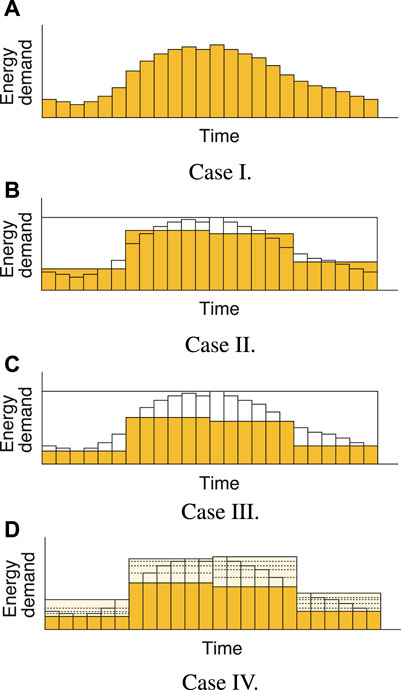
FIGURE 1. Treatment of energy demands by time series aggregation: (A) Case I; (B) Case II; (C) Case III; and (D) Case IV.

In addition, Figure 2 shows the values of the OF obtained in these cases. The numbers 1 to 3 attached in cases III and IV denote the orders in which the UB, LB, and their gap are evaluated.

FIGURE 2

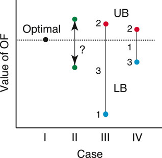
FIGURE 2. Change in the value of OF by time series aggregation.

Case I corresponds to the original optimal design problem using the original energy demands described in chapter 2. If this problem can be solved, the value of the OF will be the true optimal one. Case II corresponds to an approximate optimal design problem using the energy demands averaged for aggregated periods. Even if the value of the OF is obtained by solving this problem, it cannot be compared with the true optimal one; that is, it cannot be judged whether and how the value of the OF is larger or smaller than the true optimal one. Case III corresponds to an approximate optimal design problem using the lowest energy demands selected for aggregated periods (Bahl et al., 2018). If the value of the OF is obtained by solving this problem, it is guaranteed to be smaller than the true optimal one. This means that it can be an LB for the true optimal value of the OF. The approximate optimal design solution derived simultaneously is used to evaluate the value of the OF for the original energy demands, which becomes a UB for the true optimal value of the OF. However, since the lowest energy demands are used, it is easily guessed that the LB can be much smaller than the true optimal value of the OF, and resultantly, the gap between UB and LB can be much large. Thus, it cannot be judged whether the approximate optimal design solution is appropriate or not. In addition, to increase the LB for it to be close to the true optimal value of the OF, the number of clusters for aggregated periods must be increased. However, the approximate optimal design solution cannot coincide with the true optimal one, unless the lowest energy demands coincide with the original energy demands.

Case IV corresponds to an approximate optimal design problem by the proposed approach. In comparison with the aforementioned conventional approaches using the energy demands set in advance, the proposed approach does not fix the energy demands but can select them from their candidates for the original energy demands. In addition, even if any UB and LB are unknown, a gap between them can be evaluated and an approximate optimal design solution can be derived. To realize this, the energy demands are selected so as to keep the true optimal value of the OF within the UB and LB and minimize the gap between them. The approximate optimal design solution is used to evaluate the value of the OF for the original energy demands, which becomes a UB for the true optimal value of the OF. This is similar to the conventional approach in case III. Finally, an LB is obtained from the UB and gap. Thus, since the gap between the UB and LB is minimized, the LB can be expected to be much larger and closer to the true optimal value of the OF, even a small number of clusters for aggregated periods. In addition, there is a possibility that the approximate optimal design solution may coincide with the true optimal one even using aggregated energy demands. Therefore, it is expected that it can be judged whether the approximate optimal design solution is appropriate or not.

In the next section, the proposed approach is described theoretically.

4 Derivation and evaluation of approximate optimal design solutions

It is assumed that the number of periods M is large, and thus, the numbers of the OVs, especially integer OVs, and constraints are large in the optimal design problem of Eq. 1. In this case, it is difficult to derive the optimal design solution and evaluate the optimal value of the OF even by a commercial MILP solver.

4.1 Evaluation of design solutions

First, a design solution given a priori is evaluated; that is, it is evaluated how such a design solution is far from or close to the optimal one in terms of the value of the OF.

Although Eq. 1 may not be solved directly, the value of the OF for the optimal design solution of Eq. 1 is expressed as follows:

$F^{*}=\underset{\mathit{x}}{\min }\underset{\mathit{z}}{\min }f\left(\mathit{x},\mathit{Y},\mathit{z}\right).(3)$

On the other hand, if the values of the DVs $\tilde{\mathit{x}}$ for a design solution are given, the corresponding value of the OF is expressed as follows:

$\tilde{F}=\underset{\tilde{\mathit{z}}}{\min }f\left(\tilde{\mathit{x}},\mathit{Y},\tilde{\mathit{z}}\right).(4)$

This optimal operation problem, under the given values of the DVs $\tilde{\mathit{x}}$, can be divided into the ones for the respective periods in consideration of the independence of the OVs and constraints, and they can be solved easily. Then, the difference in the value of the OF is expressed as follows:

$\begin{array}{ll}\hfill R^{*}& =\tilde{F}-F^{*}\hfill \\ \hfill & =\underset{\tilde{\mathit{z}}}{\min }f\left(\tilde{\mathit{x}},\mathit{Y},\tilde{\mathit{z}}\right)-\underset{\mathit{x}}{\min }\underset{\mathit{z}}{\min }f\left(\mathit{x},\mathit{Y},\mathit{z}\right).\hfill \end{array}(5)$

However, since the second term on the right side of Eq. 5 cannot be evaluated, the difference of Eq. 5 can also not be evaluated.

Here, certain energy demands Y used in Eq. 5 are replaced with relaxed energy demands y which include Y, and the maximum of Eq. 5 with respect to y is evaluated as follows:

$\tilde{R}=\underset{\mathit{y}}{\max }\left(\underset{\tilde{\mathit{z}}}{\min }f\left(\tilde{\mathit{x}},\mathit{y},\tilde{\mathit{z}}\right)-\underset{\mathit{x}}{\min }\underset{\mathit{z}}{\min }f\left(\mathit{x},\mathit{y},\mathit{z}\right)\right).(6)$

Since energy demands Y are relaxed to y and the most inconvenient values are used as y, the following inequality is satisfied between Eqs. 5, 6:

$0\le R^{*}\le \tilde{R}.(7)$

This means that if $\tilde{R}$ is evaluated by Eq. 6 in place of R*, it is certified that R* cannot be larger than $\tilde{R}$. Thus, $\tilde{R}$ cannot be underestimated as an approximate difference for Eq. 5. Then, from Eqs. 5, 7, the following inequalities are satisfied for the optimal value of the OF:

$\tilde{F}-\tilde{R}\le \tilde{F}-R^{*}=F^{*}\le \tilde{F}.(8)$

These inequalities mean that even if the optimal value of the OF F* is unknown, its LB $\tilde{F}-\tilde{R}$ can be obtained. From these inequalities, it may be judged how the given design solution $\tilde{\mathit{x}}$ is far from or close to the optimal one. For this purpose, Y should be relaxed to y appropriately to reduce the differences between $\tilde{R}$ and R* as well as $\tilde{F}-\tilde{R}$ and $\tilde{F}-R^{*}$.

4.2 Aggregation of periods and energy demands

Since the operations of maximization and minimization have to be executed hierarchically in the optimization problem of Eq. 6, it becomes more complex than the ordinary optimization problem of Eq. 3, and it cannot be solved easily. Thus, time series aggregation is applied to Eq. 6; that is, all the periods are categorized into clusters of periods based on energy demands. In accordance with this clustering, the energy demands, OVs, and constraints are made common in each cluster of periods. As a result, the optimization problem of Eq. 6 is reduced and becomes easier to be solved.

As one of the general clustering methods, the k-medoids method has been applied to time series aggregation in some previous works, and it is also applied to that in this paper (Vinod, 1969). The indices m (m = 1, 2, ⋯, M) for the original periods are categorized into L sets or clusters of periods A_l (l = 1, 2, ⋯, L). First, the Euclid distance based on the energy demands for any two different original periods is calculated. Then, under the number of clusters L given as a condition, the Euclid distance between a representative period as the medoid and another period is evaluated in each cluster, and the clusters are determined to minimize the sum of the Euclid distances. If it is inappropriate to categorize some periods into a same cluster, constraints are added to categorize those periods into different clusters. This optimization problem is formulated as an integer linear programming one and can be solved using a commercial MILP solver.

With this time series aggregation of periods, the relaxed energy demands y are related with the original energy demands Y as follows:

$\mathit{y}\left(m\right)\in \left\{\mathit{Y}\left(m^{\prime }\right)|\forall m^{\prime }\in A_l\right\}\left(\forall m\in A_l;l=\mathrm{1,2},\dots ,L\right).(9)$

This means that the energy demands are common in each cluster of periods. Then, the operational strategies can also be made common by optimizing them. Thus, the energy demands and OVs for each cluster of periods are expressed as follows:

$\left.\begin{array}{c}{\mathit{y}}^{\prime }\left(l\right)=\mathit{y}\left(m\right)\hfill \\ {\mathit{z}}^{\prime }\left(l\right)=\mathit{z}\left(m\right)\hfill \\ {\tilde{\mathit{z}}}^{\prime }\left(l\right)=\tilde{\mathit{z}}\left(m\right)\hfill \end{array}\right\}\left(\forall m\in A_l;l=1,2,\cdots ,L\right),(10)$

where ( )′ denotes the values of energy demands and OVs after time series aggregation. From this relation, the energy demands after time series aggregation are selected only among the values before the time series aggregation as follows:

${\mathit{y}}^{\prime }\left(l\right)\in \left\{\mathit{Y}\left(m\right)|\forall m\in A_l\right\}\left(l=1,2,\cdots ,L\right).(11)$

This restraint minimizes the region of the energy demands y, and $\tilde{R}$ of Eq. 6 decreases as much as possible and approaches to R*.

As a result, the optimization problem of Eq. 6 is reduced to the following equation:

${\tilde{R}}^{\prime }=\underset{{\mathit{y}}^{\prime }}{\max }\left(\underset{{\tilde{\mathit{z}}}^{\prime }}{\min }f\left(\tilde{\mathit{x}},{\mathit{y}}^{\prime },{\tilde{\mathit{z}}}^{\prime }\right)-\underset{\mathit{x}}{\min }\underset{{\mathit{z}}^{\prime }}{\min }f\left(\mathit{x},{\mathit{y}}^{\prime },{\mathit{z}}^{\prime }\right)\right),(12)$

where the vectors y′, z′, and ${\tilde{\mathit{z}}}^{\prime }$ are composed of y′(l), z′(l), and ${\tilde{\mathit{z}}}^{\prime }(l)$, respectively, as follows:

$\left.\begin{array}{c}{\mathit{y}}^{\prime }={\left({\mathit{y}}^{\prime }{\left(1\right)}^{\mathrm{T}},{\mathit{y}}^{\prime }{\left(2\right)}^{\mathrm{T}},\cdots ,{\mathit{y}}^{\prime }{\left(L\right)}^{\mathrm{T}}\right)}^{\mathrm{T}}\hfill \\ {\mathit{z}}^{\prime }={\left({\mathit{z}}^{\prime }{\left(1\right)}^{\mathrm{T}},{\mathit{z}}^{\prime }{\left(2\right)}^{\mathrm{T}},\cdots ,{\mathit{z}}^{\prime }{\left(L\right)}^{\mathrm{T}}\right)}^{\mathrm{T}}\hfill \\ {\tilde{\mathit{z}}}^{\prime }={\left({\tilde{\mathit{z}}}^{\prime }{\left(1\right)}^{\mathrm{T}},{\tilde{\mathit{z}}}^{\prime }{\left(2\right)}^{\mathrm{T}},\cdots ,{\tilde{\mathit{z}}}^{\prime }{\left(L\right)}^{\mathrm{T}}\right)}^{\mathrm{T}}\hfill \end{array}\right\}.(13)$

y′ is only a concrete example of y. Thus, Eqs. 7, 8 remain valid even if ${\tilde{R}}^{\prime }$ of Eq. 12 is used in place of $\tilde{R}$ of Eq. 6.

4.3 Derivation of approximate optimal design solutions

Next, an approximate optimal design solution is derived and evaluated. Based on the aforementioned result, $\tilde{\mathit{x}}$ is treated as DVs, and ${\tilde{R}}^{\prime }$ of Eq. 12 is minimized with respect to $\tilde{\mathit{x}}$ as follows:

${\tilde{R}}^{″}=\underset{\tilde{\mathit{x}}}{\min }\underset{{\mathit{y}}^{\prime }}{\max }\left(\underset{{\tilde{\mathit{z}}}^{\prime }}{\min }f\left(\tilde{\mathit{x}},{\mathit{y}}^{\prime },{\tilde{\mathit{z}}}^{\prime }\right)-\underset{\mathit{x}}{\min }\underset{{\mathit{z}}^{\prime }}{\min }f\left(\mathit{x},{\mathit{y}}^{\prime },{\mathit{z}}^{\prime }\right)\right).(14)$

Eqs. 7, 8 remain valid even if ${\tilde{R}}^{″}$ of Eq. 14 is used in place of $\tilde{R}$ of Eq. 6. Through this optimization, ${\tilde{R}}^{″}$ can be decreased as much as possible. According to Eqs. 7, 8, this means that ${\tilde{R}}^{″}$ and $\tilde{F}-{\tilde{R}}^{″}$ approach R* and $\tilde{F}-R^{*}$, respectively, as much as possible. If ${\tilde{R}}^{″}$ and $\tilde{F}-{\tilde{R}}^{″}$ are close to zero and $\tilde{F}$, respectively, the unknown optimal value of the OF F* is bounded tightly by their UB and LB, $\tilde{F}$ and $\tilde{F}-{\tilde{R}}^{″}$, respectively, which are close to each other. Thus, it is guaranteed that the UB $\tilde{F}$ is a suitable approximate value for F* and that $\tilde{\mathit{x}}$ is a suitable approximate optimal design solution. In addition, if ${\tilde{R}}^{″}=0$, it is certified that R* = 0 and $F^{*}=\tilde{F}$, and thus, the derived approximate optimal design solution $\tilde{\mathit{x}}$ is certified to be the optimal one.

4.4 Consideration of flexibility in energy supply

The flexibility or feasibility in energy supply is not discussed in Section 4.1, Section 4.2, and Section 4.3. Since the aggregated energy demands differ from the original energy demands, design solutions $\tilde{\mathit{x}}$ and x may not satisfy the original energy demands. Thus, flexibility has to be considered for both the design solutions $\tilde{\mathit{x}}$ and x. As stated in the next section, Eqs. 12, 14 are solved by partly modifying the procedures proposed for the robust optimal design of energy supply systems under uncertain energy demands based on a mixed-integer linear model. In this robust optimal design, the flexibility is secured for all the possible values of the uncertain energy demands by introducing another objective function, which expresses the infeasibility in energy supply as a penalty term, and this objective function is minimized or made zero prior to the original objective function (Yokoyama et al., 2018). In this paper, the same approach is adopted to secure flexibility for the original energy demands. A concrete formulation is omitted here.

5 Solutions of optimization problems

5.1 Application of the robust optimization method

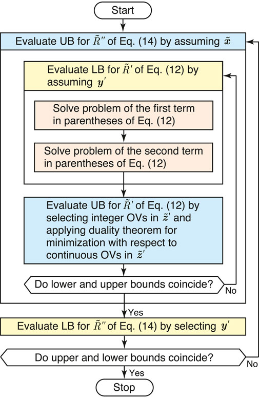
The optimization problems of Eqs. 12, 14 are bi-level and three-level MILP ones, respectively. The former has the hierarchical maximization and minimization operations with respect to the energy demands and OVs, respectively. The latter adds the minimization operation with respect to the DVs. Thus, it is difficult to solve these problems using the ordinary optimization methods. Here, they are solved by partly modifying the procedures proposed for the robust optimal design of energy supply systems under uncertain energy demands based on a mixed-integer linear model. Here, only a summary of the solutions is described as follows. For the details of the robust optimal design, refer to the work of Yokoyama et al. (2018). A flow diagram for the solutions is shown in Figure 3, where the inner and outer loops correspond to the solutions of the optimization problems of Eqs. 12, 14, respectively.

FIGURE 3

FIGURE 3. Flow diagram for solutions of optimization problems of Eqs. 12, 14.

5.1.1 Evaluation of design solutions

The optimization problem of Eq. 12 is solved as follows. First, the values of energy demands y′ in Eq. 12 are assumed, and Eq. 12 is divided into two MILP problems of the first and second terms in the parentheses, which can be solved independently using an ordinary commercial MILP solver. An LB for ${\tilde{R}}^{\prime }$ of Eq. 12 and candidate values of the integer OVs in ${\tilde{\mathit{z}}}^{\prime }$ are obtained by this procedure. Second, minimization with respect to the integer and continuous OVs in ${\tilde{\mathit{z}}}^{\prime }$ is conducted by selecting the values of the integer OVs among the ones obtained in evaluating LBs and by applying the duality theorem, respectively. In the original robust optimal design based on a mixed-integer linear model, the Karush–Kuhn–Tucker conditions have been used for minimization with respect to the continuous OVs. However, binary variables have to be added to linearize the complementarity condition by the Fortuny-Amat–McCarl approach (Fortuny-Amat and McCarl, 1981), which can lead to long computation times. Here, minimization with respect to the continuous OVs is converted to maximization with respect to their dual variables based on the duality theorem. Since the energy demands after the time series aggregation of Eq. 11 can be expressed by binary variables, the products of these dual and binary variables are linearized by adding linear inequalities by the Glover approach (Glover, 1975). Thus, this conversion is effective to solve such a type of bi-level MILP problems (Zare et al., 2019) and has been applied to a bi-level linear programming problem for the robust optimal design based on a linear model in consideration of its features (Yokoyama et al., 2014). The resultant optimization problem is also an MILP one, which can be solved using an ordinary commercial MILP solver. A UB for ${\tilde{R}}^{\prime }$ of Eq. 12 and candidate values of the energy demands y′ for the next iteration are obtained by this procedure. Through these procedures, UBs and LBs for ${\tilde{R}}^{\prime }$ of Eq. 12 are evaluated alternately and repeatedly until they coincide with each other.

5.1.2 Derivation of approximate optimal design solutions

The optimization problem of Eq. 14 is solved as follows. First, the values of the DVs $\tilde{\mathit{x}}$ in Eq. 14 are assumed, and then, Eq. 14 is reduced to Eq. 12, which can be solved as mentioned previously. A UB for ${\tilde{R}}^{″}$ of Eq. 14 and candidate values of the energy demands y′ are obtained by this procedure. Second, Eq. 14 is relaxed by selecting the values of y′ among the ones obtained in evaluating UBs. This optimization problem results in an MILP problem, which can be solved using an ordinary commercial MILP solver. An LB for ${\tilde{R}}^{″}$ of Eq. 14 and candidate values of the DVs $\tilde{\mathit{x}}$ for the next iteration are obtained by this procedure. Using these procedures, UBs and LBs for ${\tilde{R}}^{″}$ of Eq. 14 are evaluated alternately and repeatedly until they coincide with each other.

5.2 Application of the hierarchical optimization method

As mentioned previously, three MILP problems of different types have to be solved repeatedly to solve the optimization problem of Eq. 12. Also, another MILP problem of a different type has to be solved repeatedly to solve the optimization problem of Eq. 14. One of these four MILP problems has only the OVs, and it can be solved easily. However, three of them have both the DVs and OVs, and they cannot be solved easily when the configuration of the energy supply system is complex and the number of periods is still large, even after time series aggregation. This is because the OVs for all the periods are related through the DVs and the problem can be large scale. A hierarchical MILP method has been proposed to solve the ordinary optimal design problems efficiently (Yokoyama et al., 2015). In addition, this method has been applied to the robust optimal design (Yokoyama et al., 2021). In this paper, the method is applied to solve the three MILP problems with both the DVs and OVs. Since the three MILP problems are of different types, the original hierarchical MILP method is applied to each problem without and with its modification. For the details of the hierarchical MILP method and its application to the robust optimal design, refer to the work of Yokoyama et al. (2015) and Yokoyama et al. (2021).

6 Case study

6.1 Input data

A gas turbine cogeneration system with a practical configuration for district energy supply is dealt with in the case study, and the proposed approach is applied to its optimal design. The configuration of this system is shown in Figure 4. Since another purpose of this paper is to show the effectiveness of the proposed approach for time series aggregation, the system treated for the case study is conventional, and not only the optimal but also the 2nd to 1000th best design solutions have been known by the work of Yokoyama et al. (2019a). The conditions for the optimal design are described in brief as follows by taking its original versions from this reference and modifying them slightly for the purpose of this paper.

FIGURE 4

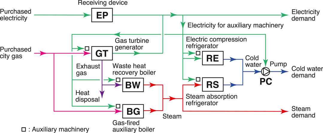
FIGURE 4. Configuration of the gas turbine cogeneration system.

“The super structure for the gas turbine cogeneration system is composed of gas turbine generators (GTs), waste heat recovery boilers (BWs), gas-fired auxiliary boilers (BGs), electric compression refrigerators (REs), steam absorption refrigerators (RSs), a receiving device for purchasing electricity (EP), and pumps for supplying cold water (PCs). The capacities for candidates of the equipment for selection are shown together with their representative performance characteristic values in Table 1. The maximum demands of purchased energy are selected among their discrete values. The annual total cost is adopted as the objective function. The capital unit costs of the equipment are shown together with the unit costs for demand and energy charges of purchased energy in Table 2. Other design conditions are summarized in Table 3”.

TABLE 1

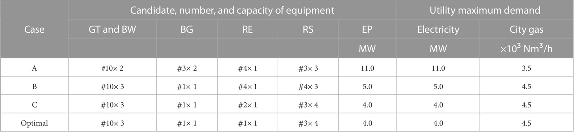
TABLE 1. Values of DVs for design solutions.

TABLE 2

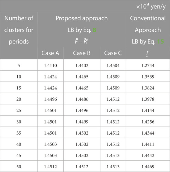
TABLE 2. LBs for the optimal value of OF for design solutions.

TABLE 3

TABLE 3. Values of DVs for the approximate optimal design solutions by the proposed approach.

Here, Tables 1–3 are the ones included in the work of Yokoyama et al. (2019a). A part of the formulation of this optimal design problem is described in Supplementary Appendix SA1, and a set of input data for the optimization calculation is shown in Supplementary Appendix SA2.

Seasonal and hourly variations in electricity, cold water, and steam demands estimated originally are shown in green lines in Figures 5A–C, respectively. The number of the clusters for periods is changed as L = 5 to 50, and the periods and energy demands are aggregated under each value of L. Since the unit costs for energy charge of purchased electricity are different in summer and other seasons, the periods in summer and other seasons are categorized into different clusters. In addition, the operation of refrigerators is necessary and unnecessary for non-zero and zero cold water demands, respectively, and the periods in mid-season with non-zero and zero cold water demands are categorized into different clusters.

FIGURE 5

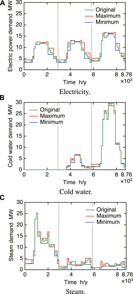
FIGURE 5. Seasonal and hourly variations in original and aggregated energy demands (L = 20): (A) electricity; (B) cold water; and (C) steam.

Since the system configuration is rather complex, the optimization calculation by the proposed approach is conducted with the aid of the hierarchical optimization method. To show how the proposed approach is effective, the values of DVs as well as UBs and LBs for the optimal value of the OF are also derived by the conventional approach proposed by Bahl et al. (2018) and modified slightly. In this approach, the energy demands for clustered periods which minimize the OF are adopted, and the values of DVs $\underset{̃}{\mathit{x}}$ and an LB $\underset{̃}{F}$ for the unknown optimal value of the OF F* are obtained by solving the following optimization problem:

$\underset{̃}{F}=\underset{\underset{̃}{\mathit{x}}}{\min }\underset{{\mathit{y}}^{\prime }}{\min }\underset{{\underset{̃}{\mathit{z}}}^{\prime }}{\min }f\left(\underset{̃}{\mathit{x}},{\mathit{y}}^{\prime },{\underset{̃}{\mathit{z}}}^{\prime }\right).(15)$

This method can increase the LB even slightly as compared with that obtained by Bahl et al. (2018). Although the optimization problem of Eq. 15 includes the DVs and OVs, it can be solved easily because of the aggregated periods and energy demands. The flexibility or feasibility in the energy supply for the original energy demands is secured by the approach stated in Section 4.4. In addition, a UB $\tilde{F}$ for the unknown optimal value of the OF F* is determined by solving the following optimization problem:

$\tilde{F}=\underset{\underset{̃}{\mathit{z}}}{\min }f\left(\underset{̃}{\mathit{x}},\mathit{Y},\underset{̃}{\mathit{z}}\right).(16)$

This is the optimal operation problem under the given values of the DVs $\underset{̃}{\mathit{x}}$, and it can be solved easily.

IBM ILOG CPLEX Optimization Studio Ver. 12.10.0 is used as a commercial MILP solver to execute all the optimization calculations necessary for the proposed and conventional approaches on an iMac Pro with Intel Xeon W processor (10 cores and 3.0 GHz) (IBM Corporation, 2019).

6.2 Results and discussion

6.2.1 Aggregation of periods and energy demands

First, the results obtained by aggregating periods and energy demands are shown. Figure 6 shows the load duration curves of the maxima and minima for the aggregated energy demands in case of the number of clusters L = 20 as an example. The maxima and minima for the aggregated energy demands are arranged in the descending order of the average energy demands. This figure also includes the original energy demands arranged in their descending order in each cluster. Figures (A) to (C) correspond to the electricity, cold water, and steam demands, respectively. As a result, the orders of the clusters in figures (A) to (C) differ from one another. Figures 5A–C also include seasonal and hourly variations in the maxima and minima for the aggregated energy demands. From these figures, it turns out that although the widths between the maxima and minima for the aggregated energy demands and the numbers of periods in clusters depend on clusters, clustering is conducted appropriately in consideration of the magnitudes of the original electricity, cold water, and steam demands. Thus, the maxima and minima for the aggregated energy demands are determined appropriately.

FIGURE 6

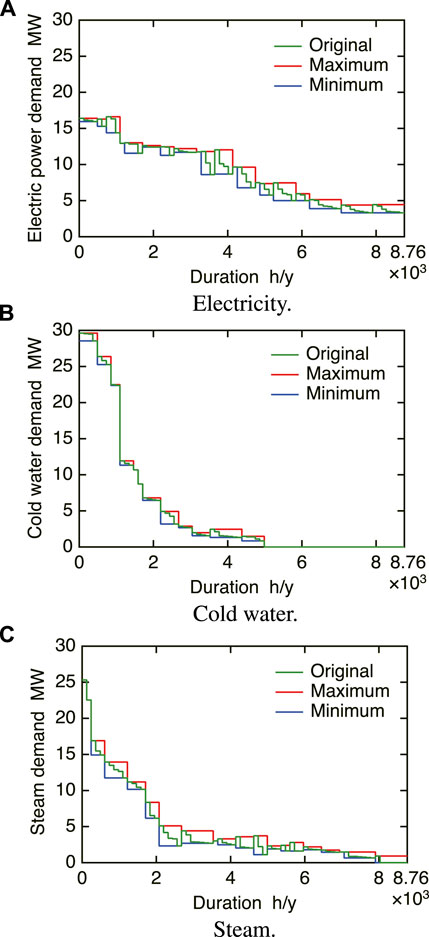
FIGURE 6. Load duration curves for the original and aggregated energy demands (L = 20): (A) electricity; (B) cold water; and (C) steam.

6.2.2 Evaluation of design solutions

Next, the results obtained by evaluating LBs for the optimal value of the OF are shown in three cases, namely, A to C, when the number of clusters is changed as L = 5 to 50. Table 1 shows the values of the DVs for the design solutions given a priori in these cases and the optimal design solution. Here, the optimal design solution has been obtained by Yokoyama et al. (2019a). In the order of cases, A to C, the design solutions approach the optimal one. The values of the OF for the design solutions are evaluated by solving the optimal operation problem of Eq. 4 for the original energy demands, using the given values of the DVs. The LBs for the optimal value of the OF in the proposed approach are obtained by Eq. 8 using the gaps between UBs and LBs obtained by Eq. 12. The LBs for the optimal value of the OF in the conventional approach are calculated by Eq. 15. The values of the OF by Eq. 4 for the design solutions in cases A to C are $\tilde{F}=$ 1.5249, 1.4875, and 1.4667 ×10⁹ yen/y, respectively. Table 2 shows the LBs for the optimal value of the OF in cases A to C evaluated by the proposed approach and those in all the cases evaluated by the conventional approach. Figures 7A–C also show these values in cases A to C, respectively. Here, the increase or decrease rate in the OF is adopted as the longitudinal axis with its reference value F* =1.4513 ×10⁹ yen/y corresponding to the optimal design solution.

FIGURE 7

FIGURE 7. Values of OF and LBs for the optimal value of OF evaluated using design solutions: (A) Case A; (B) Case B; and (C) Case C.

Since the design solutions are given a priori, the values of the OF are constant regardless of the number of clusters L in the transverse axis. The LBs evaluated by the proposed approach are very close to the optimal value of the OF in most of the design solutions and the numbers of clusters, and the validity of the proposed approach is clarified. As the aggregation rate becomes high and the number of clusters decreases, the LB tends to decrease and becomes far from the optimal value of the OF. However, as the design solutions approach the optimal one, this tendency becomes weak. This suggests that the proposed approach may derive suitable approximate optimal design solutions with the UBs and LBs, which tightly bound the optimal value of the OF. On the other hand, the LB evaluated by the conventional approach increases with the number of clusters and approaches the optimal value of the OF. However, the LBs evaluated by the conventional approach are much smaller than those by the proposed approach in all the numbers of clusters. This feature does not depend on the design solutions because the LBs are evaluated independently of the design solutions and dependently only on the energy demands.

6.2.3 Derivation of approximate optimal design solutions

Next, the results obtained by deriving the approximate optimal design solutions and evaluating UBs and LBs for the optimal value of the OF are shown, when the number of clusters is changed as L = 5 to 50. Tables 3, 4 show the values of the DVs for the approximate optimal design solutions obtained by the proposed and conventional approaches, respectively, and the optimal design solution. The UBs for the optimal value of the OF in the proposed and conventional approaches are evaluated by solving the optimal operation problems of Eqs. 4, 16 for the original energy demands, using the values of the DVs for the approximate optimal design solutions obtained by Eqs. 14, 15, respectively. The LBs for the optimal value of the OF in the proposed approach are calculated by Eq. 8 using the gaps between UBs and LBs obtained simultaneously in deriving the approximate optimal design solutions. The LBs for the optimal value of the OF in the conventional approach are calculated by Eq. 15. Table 5 shows the UBs and LBs for the optimal value of the OF corresponding to the approximate optimal design solutions obtained by the proposed and conventional approaches. Figure 8 shows these values. Here, the increase or decrease rate in the OF is adopted as the longitudinal axis with its reference value F* =1.4513 ×10⁹ yen/y corresponding to the optimal design solution.

TABLE 4

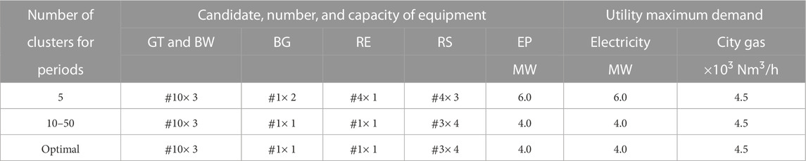
TABLE 4. Values of DVs for the approximate optimal design solutions by the conventional approach.

TABLE 5

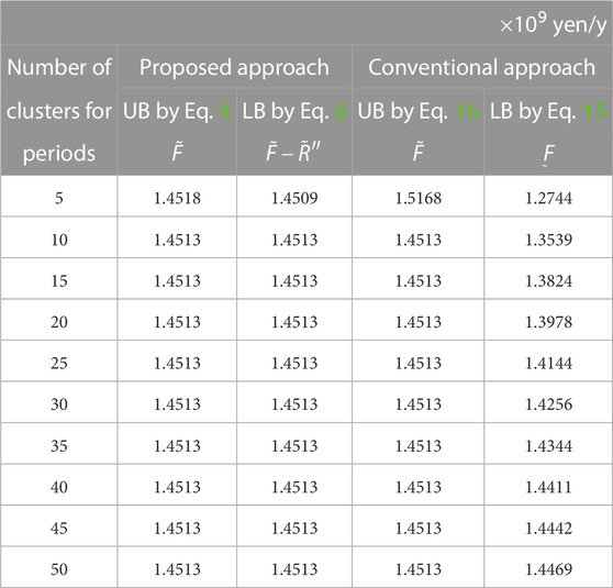
TABLE 5. UBs and LBs for the optimal value of OF for the approximate optimal design solutions.

FIGURE 8

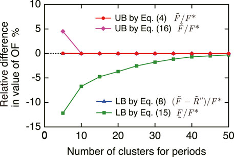
FIGURE 8. UBs and LBs for the optimal value of OF evaluated using the approximate optimal design solutions.

The optimal design solutions are obtained as the approximate ones in cases of L = 10 to 50 by both the proposed and conventional approaches, and thus, the UBs coincide with the optimal value of the OF. In case of L = 5, the approximate optimal design solutions, different from the optimal one, are derived by both the proposed and conventional approaches. Although the UB obtained by the conventional approach is much larger than the optimal value of the OF, the one obtained by the proposed approach is only slightly larger. According to Yokoyama et al. (2019a), the approximate optimal solution obtained by the conventional approach is inferior to the 1000th best solution, while the one obtained by the proposed approach is the 2nd best solution. On the other hand, the LBs obtained by the proposed approach differ significantly from those by the conventional approach, which are the same as those in Figure 7. In the proposed approach, the LBs coincide with the UBs in cases of L = 10 to 50, and thus, the optimality of the approximate optimal design solutions is guaranteed. In addition, the gap between the UB and LB is very small, even in the case of L = 5, and thus, it is guaranteed that the approximate optimal design solution is very close to the optimal one. This is because the gaps between UBs and LBs are evaluated directly using the aggregated energy demands. In the conventional approach, however, the gap decreases with an increase in the number of clusters, but the UBs and LBs never coincide with each other. This is because the UBs and LBs are evaluated using different energy demands. As a result, if time series aggregation is applied, the UBs and LBs cannot coincide with each other. For example, the LB in case of L = 50 by the conventional approach is smaller than that in case of L = 5 by the proposed approach. Therefore, to guarantee a same degree of gap, the proposed approach can heighten the aggregation rate as compared with the conventional approach.

6.2.4 Computation times for optimization calculations

Finally, the computation times for the optimization calculations in the proposed approach are investigated, and their examples are shown here. The numbers of clusters for periods L = 10, 30, and 50 are selected as examples. In addition, the values of the DVs for the design solutions given a priori in case B are selected as the initial values of the DVs to derive the approximate optimal design solutions. Tables 6a–c show the total and breakdown of the computation times for L = 10, 30, and 50, respectively. Since the optimization problems of Eqs. 12, 14 are solved as shown in Figure 3, the breakdown of the computation times is shown according to the flow of the solutions. Only the 1st outer iteration corresponds to the solution of Eq. 12 to evaluate the design solutions, and the whole corresponds to the solution of Eq. 14 to derive the approximate optimal design solutions. The computation times to evaluate LB for ${\tilde{R}}^{\prime }$ and LB for ${\tilde{R}}^{″}$ are relatively short and decrease with a decrease in L. This is because the number of periods decreases. On the other hand, the computation times to evaluate UB for ${\tilde{R}}^{\prime }$ are relatively long and tend to increase with a decrease in L. This is because although the number of periods decreases, the number of candidate values of the energy demands in each period increases, which complicates the corresponding MILP problem. In addition, the numbers of the inner and outer iterations tend to increase with a decrease in L. For comparison, the optimal design problem with the original energy demands for 72 periods is solved by the commercial MILP solver only. The UBs and LBs do not coincide even in a long computation time. For example, the UBs and LBs are 1.4513 and 1.4481 ×10⁹ yen/y, respectively, and their gap 0.22% remains in 1,200 s, which is longer than the total computation times shown in Table 6. The comparison of this LB and the ones shown in Tables 2, 5 indicates the effectiveness of the proposed approach. This is because the hierarchical optimization method makes the optimization calculation in the proposed approach possible in practical computation times.

TABLE 6

TABLE 6. Computation times for optimization calculations in the proposed approach: (a)L = 10; (b)L = 30; and (c)L = 50.

7 Conclusions

An effective approach for time series aggregation has been proposed to derive an approximate optimal design solution and evaluate the gap between the UB and LB for the optimal value of OF in an optimal design problem of the energy supply systems based on a mixed-integer linear model. First, an approach for evaluating a design solution has been presented, and it has been followed by an approach for deriving an approximate optimal design solution and evaluating it. The optimization problems for these purposes have been treated as bi-level and three-level MILP problems, and they have been solved by the aid of the robust optimization method. In addition, the hierarchical optimization method has been applied for them to be solved in practical computation times.

A case study has been carried out on the optimal design of a cogeneration system with a practical configuration to show how the proposed approach is effective in comparison with a conventional approach. The study has led to the following main results:

•In most of the cases for design solutions and numbers of clusters for aggregated periods, the proposed approach can evaluate LBs close to the optimal value of the OF, and thus, it can be evaluated suitably how design solutions are far from or close to the optimal one.

•In most of the numbers of clusters for aggregated periods, the proposed approach can evaluate UBs and LBs equal to the optimal value of the OF, and thus, can derive the approximate optimal design solutions which are certified to be the optimal one. Even in other cases, the proposed approach can evaluate UBs and LBs close to the optimal value of the OF, and thus, derive suitable approximate optimal design solutions close to the optimal one.

•In most of the numbers of clusters for aggregated periods, the conventional approach can also evaluate UBs equal to the optimal value of the OF, but it evaluates much smaller LBs as compared with the proposed approach. In other cases, the conventional approach evaluates much larger UBs and much smaller LBs as compared with the proposed approach.

•Form these results, the proposed approach surpasses the conventional one in evaluating small gaps between UBs and LBs, and thus, it can reduce the number of clusters for aggregated periods significantly for time series aggregation.

In this paper, it has been assumed that the energy supply systems do not include any energy storage units. However, the proposed method will be extended for systems with energy storage units for their short-term cyclic operation by modifying the time series aggregation. This work will be conducted in the future.

Data availability statement

The original contributions presented in the study are included in the article/Supplementary Material. Further inquiries can be directed to the corresponding author.

Author contributions

RY was involved in conceptualization, methodology, software, formal analysis, investigation, resources, data curation, visualization, writing—original draft preparation, writing—reviewing and editing, supervision, and funding acquisition. YS was involved in software, formal analysis, writing—reviewing and editing, and funding acquisition. TW was involved in validation, resources, and writing—reviewing and editing. All authors contributed to the article and approved the submitted version.

Funding

A part of the work in this paper has been conducted with support by the JSPS Grant-in-Aid for Scientific Research (KAKENHI) (C) No. 18K05017 and the Research Campus Modal funded by the German Federal Ministry of Education and Research No. 05M20ZBM. This support is greatly acknowledged.

Acknowledgments

A part of the work in this paper has been conducted with support by the IBM Academic Initiative. This support is greatly acknowledged.

Conflict of interest

The authors declare that the research was conducted in the absence of any commercial or financial relationships that could be construed as a potential conflict of interest.

Publisher’s note

All claims expressed in this article are solely those of the authors and do not necessarily represent those of their affiliated organizations, or those of the publisher, the editors, and the reviewers. Any product that may be evaluated in this article, or claim that may be made by its manufacturer, is not guaranteed or endorsed by the publisher.

Supplementary material

The Supplementary Material for this article can be found online at: https://www.frontiersin.org/articles/10.3389/fenrg.2023.1128681/full#supplementary-material

References

Andiappan, V. (2017). State-of-the-art review of mathematical optimisation approaches for synthesis of energy systems. Process Integration Optim. Sustain.1, 165–188. doi:10.1007/s41660-017-0013-2

CrossRef Full Text | Google Scholar

Bahl, B., Kümpel, A., Seele, H., Lampe, M., and Bardow, A. (2017). Time-series aggregation for synthesis problems by bounding error in the objective function. Energy135, 900–912. doi:10.1016/j.energy.2017.06.082

CrossRef Full Text | Google Scholar

Bahl, B., Lützow, J., Shu, D., Hollermann, D. E., Lampe, M., Hennen, M., et al. (2018). Rigorous synthesis of energy systems by decomposition via time-series aggregation. Comput. Chem. Eng.112, 70–81. doi:10.1016/j.compchemeng.2018.01.023

CrossRef Full Text | Google Scholar

Baumgärtner, N., Bahl, B., Hennen, M., and Bardow, A. (2019a). RiSES³: Rigorous Synthesis of Energy Supply and Storage Systems via time-series relaxation and aggregation. Comput. Chem. Eng.127, 127–139. doi:10.1016/j.compchemeng.2019.02.006

CrossRef Full Text | Google Scholar

Baumgärtner, N., Temme, F., Bahl, B., Hennen, M., Hollermann, D., and Bardow, A. (2019b). “RiSES⁴ Rigorous Synthesis of Energy Supply Systems with Seasonal Storage by relaxation and time-series aggregation to typical periods,” in Proceeding of the 32nd international conference on efficiency, cost, optimization, simulation and environmental impact of energy systems (ECOS 2019).263–274.

Google Scholar

Buoro, D., Casisi, M., De Nardi, A., Pinamonti, P., and Reini, M. (2013). Multicriteria optimization of a distributed energy supply system for an industrial area. Energy58, 128–137. doi:10.1016/j.energy.2012.12.003

CrossRef Full Text | Google Scholar

Buoro, D., Casisi, M., Pinamonti, P., and Reini, M. (2012). Optimal synthesis and operation of advanced energy supply systems for standard and domotic home. Energy Convers. Manag.60, 96–105. doi:10.1016/j.enconman.2012.02.008

CrossRef Full Text | Google Scholar

Carvalho, M., Serra, L. M., and Lozano, M. A. (2011). Optimal synthesis of trigeneration systems subject to environmental constraints. Energy36, 3779–3790. doi:10.1016/j.energy.2010.09.023

CrossRef Full Text | Google Scholar

Domínguez-Muñoz, F., Cejudo-López, J. M., Carrillo-Andrés, A., and Gallardo-Salazar, M. (2011). Selection of typical demand days for CHP optimization. Energy Build.43, 3036–3043. doi:10.1016/j.enbuild.2011.07.024

CrossRef Full Text | Google Scholar

Fazlollahi, S., Bungener, S. L., Mandel, P., Becker, G., and Maréchal, F. (2014). Multi-objectives, multi-period optimization of district energy systems: I. Selection of typical operating periods. Comput. Chem. Eng.65, 54–66. doi:10.1016/j.compchemeng.2014.03.005

CrossRef Full Text | Google Scholar

Fortuny-Amat, J., and McCarl, B. (1981). A representation and economic interpretation of a two-level programming problem. J. Operational Res. Soc.32, 783–792. doi:10.2307/2581394

CrossRef Full Text | Google Scholar

Frangopoulos, C. A. (2018). Recent developments and trends in optimization of energy systems. Energy164, 1011–1020. doi:10.1016/j.energy.2018.08.218

CrossRef Full Text | Google Scholar

Ganschinietz, C. (2021). Design of on-site energy conversion systems for manufacturing companies—a concept-centric research framework. J. Clean. Prod.310, 1–20, Paper No. 127258. doi:10.1016/j.jclepro.2021.127258

CrossRef Full Text | Google Scholar

Glover, F. (1975). Improved linear integer programming formulations of nonlinear integer problems. Manag. Sci.22, 455–460. doi:10.1287/mnsc.22.4.455

CrossRef Full Text | Google Scholar

Goderbauer, S., Comis, M., and Willamowski, F. J. L. (2019). The synthesis problem of decentralized energy systems is strongly NP-hard. Comput. Chem. Eng.124, 343–349. doi:10.1016/j.compchemeng.2019.02.002

CrossRef Full Text | Google Scholar

Guepa, E., Bischi, A., Verda, V., Chertkof, M., and Lund, H. (2019). Towards future infrastructures for sustainable multi-energy systems: A review. Energy184, 2–21. doi:10.1016/j.energy.2019.05.057

CrossRef Full Text | Google Scholar

Hoffmann, M., Kotzur, L., Stolten, D., and Robinius, M. (2020). A review on time series aggregation methods for energy system models. Energies13, 1–71. Paper No. 641. doi:10.3390/en13030641

CrossRef Full Text | Google Scholar

Horii, S., Ito, K., Pak, P. S., and Suzuki, Y. (1987). Optimal planning of gas turbine co-generation plants based on mixed-integer linear programming. Int. J. Energy Res.11, 507–518. doi:10.1002/er.4440110407

CrossRef Full Text | Google Scholar

IBM Corporation (2019). IBM ILOG CPLEX optimization Studio V12.10.0 documentation.

Google Scholar

Iyer, R. R., and Grossmann, I. E. (1998). Synthesis and operational planning of utility systems for multiperiod operation. Comput. Chem. Eng.22, 979–993. doi:10.1016/s0098-1354(97)00270-6

CrossRef Full Text | Google Scholar

Kannengießer, T., Hoffmann, M., Kotzur, L., Stenzel, P., Schuetz, F., Peters, K., et al. (2019). Reducing computational load for mixed integer linear programming: An example for a district and an island energy system. Energies12, 1–27. Paper No. 2825. doi:10.3390/en12142825

CrossRef Full Text | Google Scholar

Kotzer, L., Nolting, L., Hoffmann, M., Groß, T., Smolenko, A., Priesmann, J., et al. (2021). A modeler’s guide to handle complexity in energy system optimization. Adv. Appl. Energy4. 1–19, Paper No. 100063. doi:10.1016/j.adapen.2021.100063

CrossRef Full Text | Google Scholar

Kotzur, L., Markewitz, P., Robinius, M., and Stolten, D. (2018). Impact of different time series aggregation methods on optimal energy system design. Renew. Energy117, 474–487. doi:10.1016/j.renene.2017.10.017

CrossRef Full Text | Google Scholar

Lin, F., Leyffer, S., and Munson, T. (2016). A two-level approach to large mixed-integer programs with application to cogeneration in energy-efficient buildings. Comput. Optim. Appl.65, 1–46. doi:10.1007/s10589-016-9842-0

CrossRef Full Text | Google Scholar

Lozano, M. A., Ramos, J. C., Carvalho, M., and Serra, L. M. (2009). Structure optimization of energy supply systems in tertiary sector buildings. Energy Build.41, 1063–1075. doi:10.1016/j.enbuild.2009.05.008

CrossRef Full Text | Google Scholar

Lozano, M. A., Ramos, J. C., and Serra, L. M. (2010). Cost optimization of the design of CHCP (combined heat, cooling and power) systems under legal constraints. Energy35, 794–805. doi:10.1016/j.energy.2009.08.022

CrossRef Full Text | Google Scholar

Lythcke-Jørgensen, C., Münster, M., Ensinas, A. V., and Haglind, F. (2016). A method for aggregating external operating conditions in multi-generation system optimization models. Appl. Energy166, 59–75. doi:10.1016/j.apenergy.2015.12.050

CrossRef Full Text | Google Scholar

Mancarella, P. (2014). MES (multi-energy systems): An overview of concepts and evaluation models. Energy65, 1–17. doi:10.1016/j.energy.2013.10.041

CrossRef Full Text | Google Scholar

Nahmmacher, P., Schmid, E., Hirth, L., and Knopf, B. (2016). Carpe diem: A novel approach to select representative days for long-term power system modeling. Energy112, 430–442. doi:10.1016/j.energy.2016.06.081

CrossRef Full Text | Google Scholar

Piacentino, A., Barbaro, C., Cardona, F., Gallea, R., and Cardona, E. (2013). A comprehensive tool for efficient design and operation of polygeneration-based energy grids serving a cluster of buildings. Part I: Description of the method. Appl. Energy111, 1204–1221. doi:10.1016/j.apenergy.2012.11.078

CrossRef Full Text | Google Scholar

Poncelet, K., Höschle, H., Delarue, E., Virag, A., and D’haeseleer, W. (2017). Selecting representative days for capturing the implications of integrating intermittent renewables in generation expansion planning problems. IEEE Trans. Power Syst.32, 1936–1948. doi:10.1109/tpwrs.2016.2596803

CrossRef Full Text | Google Scholar

Rech, S. (2019). Smart energy systems: Gudelines for modeling and optimizing a fleet of units of different configurations. Energies12, 1–36. Paper No. 1320. doi:10.3390/en12071320

CrossRef Full Text | Google Scholar

Ringkjøb, H.-K., Haugan, P. M., and Solbrekke, I. M. (2018). A review of modelling tools for energy and electricity systems with large shares of variable renewables. Renew. Sustain. Energy Rev.96, 440–459. doi:10.1016/j.rser.2018.08.002

CrossRef Full Text | Google Scholar

Schütz, T., Schraven, M. H., Fuchs, M., Remmen, P., and Müller, D. (2018). Comparison of clustering algorithms for the selection of typical demand days for energy system synthesis. Renew. Energy129, 570–582. doi:10.1016/j.renene.2018.06.028

CrossRef Full Text | Google Scholar

Scott, I. J., Carvalho, P. M. S., Botterud, A., and Silva, C. A. (2019). Clustering representative days for power systems generation expansion planning: Capturing the effects of variable renewables and energy storage. Appl. Energy253, 1–17. Paper No. 113603. doi:10.1016/j.apenergy.2019.113603

CrossRef Full Text | Google Scholar

Teichgraeber, H., and Brandt, A. R. (2019). Clustering methods to find representative periods for the optimization of energy systems: An initial framework and comparison. Appl. Energy239, 1283–1293. doi:10.1016/j.apenergy.2019.02.012

CrossRef Full Text | Google Scholar

Teichgraeber, H., and Brandt, A. R. (2022). Time-series aggregation for the optimization of energy systems: Goals, challenges, approaches, and opportunities. Renew. Sustain. Energy Rev.157, 1–17. Paper No. 111984. doi:10.1016/j.rser.2021.111984

CrossRef Full Text | Google Scholar

Vinod, H. D. (1969). Integer programming and the theory of grouping. J. Am. Stat. Assoc.64, 506–519. doi:10.1080/01621459.1969.10500990

CrossRef Full Text | Google Scholar

Voll, P., Hennen, M., Klaffke, C., Lampe, M., and Bardow, A. (2013a). Exploring the near-optimal solution space for the synthesis of distributed energy supply systems. Chem. Eng. Trans.35, 277–282. doi:10.3303/CET1335046

CrossRef Full Text | Google Scholar

Voll, P., Klaffke, C., Hennen, M., and Bardow, A. (2013b). Automated superstructure-based synthesis and optimization of distributed energy supply systems. Energy50, 374–388. doi:10.1016/j.energy.2012.10.045

CrossRef Full Text | Google Scholar

Wakui, T., and Yokoyama, R. (2014). Optimal structural design of residential cogeneration systems in consideration of their operating restrictions. Energy64, 719–733. doi:10.1016/j.energy.2013.10.002

CrossRef Full Text | Google Scholar

Yokoyama, R., Fujiwara, K., Ohkura, H., and Wakui, T. (2014). A revised method for robust optimal design of energy supply systems based on minimax regret criterion. Energy Convers. Manag.84, 196–208. doi:10.1016/j.enconman.2014.03.045

CrossRef Full Text | Google Scholar

Yokoyama, R., Hasegawa, Y., and Ito, K. (2002). A MILP decomposition approach to large scale optimization in structural design of energy supply systems. Energy Convers. Manag.43, 771–790. doi:10.1016/s0196-8904(01)00075-9

CrossRef Full Text | Google Scholar

Yokoyama, R., and Ito, K. (2006). Optimal design of gas turbine cogeneration plants in consideration of discreteness of equipment capabilities. Trans. ASME, J. Eng. Gas Turbines Power128, 336–343. doi:10.1115/1.2131889

CrossRef Full Text | Google Scholar

Yokoyama, R., Kamada, H., Shinano, Y., and Wakui, T. (2021). A hierarchical optimization approach to robust design of energy supply systems based on a mixed-integer linear model. Energy229, 1–12. Paper No. 120343. doi:10.1016/j.energy.2021.120343

CrossRef Full Text | Google Scholar

Yokoyama, R., and Shinano, Y. (2015). “MILP approaches to optimal design and operation of distributed energy systems,” in Optimization in the real world—toward solving real world optimization problems. Editors K. Fujisawa, Y. Shinano, and H. Waki (Tokyo: Springer), 157–176.

CrossRef Full Text | Google Scholar

Yokoyama, R., Shinano, Y., Taniguchi, S., Ohkura, M., and Wakui, T. (2015). Optimization of energy supply systems by MILP branch and bound method in consideration of hierarchical relationship between design and operation. Energy Convers. Manag.92, 92–104. doi:10.1016/j.enconman.2014.12.020

CrossRef Full Text | Google Scholar

Yokoyama, R., Shinano, Y., Taniguchi, S., and Wakui, T. (2019a). Search for K-best solutions in optimal design of energy supply systems by an extended MILP hierarchical branch and bound method. Energy184, 45–57. doi:10.1016/j.energy.2018.02.077

CrossRef Full Text | Google Scholar

Yokoyama, R., Shinano, Y., Wakayama, Y., and Wakui, T. (2019b). Model reduction by time aggregation for optimal design of energy supply systems by an MILP hierarchical branch and bound method. Energy181, 782–792. doi:10.1016/j.energy.2019.04.066

CrossRef Full Text | Google Scholar

Yokoyama, R., Tokunaga, A., and Wakui, T. (2018). Robust optimal design of energy supply systems under uncertain energy demands based on a mixed-integer linear model. Energy153, 159–169. doi:10.1016/j.energy.2018.03.124

CrossRef Full Text | Google Scholar

Zare, M. H., Borrero, J. S., Zeng, B., and Prokopyev, O. A. (2019). A note on linearized reformulations for a class of bilevel linear integer problems. Ann. Operations Res.272, 99–117. doi:10.1007/s10479-017-2694-x

CrossRef Full Text | Google Scholar

Zatti, M., Gabba, M., Freschini, M., Rossi, M., Gambarotta, A., Morini, M., et al. (2019). k-MILP: A novel clustering approach to select typical and extreme days for multi-energy systems design optimization. Energy181, 1051–1063. doi:10.1016/j.energy.2019.05.044

CrossRef Full Text | Google Scholar

Zhou, Z., Liu, P., Li, Z., and Ni, W. (2013). An engineering approach to the optimal design of distributed energy systems in China. Appl. Therm. Eng.53, 387–396. doi:10.1016/j.applthermaleng.2012.01.067

CrossRef Full Text | Google Scholar