Intelligent Decoupling Control Study of PMSM Based on the Neural Network Inverse System

This study obtains the analytical inverse system of a permanent magnet synchronous motor (PMSM) model based on the traditional magnetic field orientation decoupling control mode by analyzing the inverse quality of the PMSM. Using the neural network’s excellent approximation ability and well learning functions, a neural network inverse system (NNIS) of the decoupling control system was established by identifying and offline training the back propagation neural network (BPNN) and radial basis function neural network (RBFNN). The data collected from the analytical inverse system of the PMSM model are used to analyze and compare the prediction accuracy and running time of the neural network, so as to optimize the structure and parameters of the neural network. The simulation results of three PMSM decoupling control systems show that the PMSM decoupling control system based on RBF NNIS has good dynamic and static decoupling performance, and robustness.

Introduction

PMSM is an efficient and energy-saving motor, and it is a nonlinear, multivariable, and strongly coupled control object (Bu et al., 2015; Sun et al., 2016; Bu et al., 2019a). The control effect of traditional motor control methods is not ideal. Various control methods of modern motors are essentially decoupling control. At present, the industry adopts field-oriented control to realize decoupling control through id = 0. This is a decoupling method based on an accurate mathematical model, which has good performance in steady-state decoupling. However, the system performance in the dynamic process and when the motor parameters change is not very ideal, and intelligent control is the development trend in the future. This kind of the control method does not have high requirements for the mathematical model. At present, it has many successful applications (Li et al., 2019a; Jie et al., 2020), such as NNIS. This method is an important branch of intelligent decoupling control of the PMSM.

In the decoupling strategy of the NNIS, the key is the design and construction of the neural network, but the relevant research and literature have not been discussed too much. A typical error in the back-propagation feed-forward neural network (BPNN) is selected in many documents to identify the inverse system (Bu et al., 2019b; Xie and Xie, 2020). There is no detailed description on how to select the parameters and algorithm in the BPNN. Similarly, RBFNN with good approximation and fitting ability has not been used to identify the inverse system, let alone compare the decoupling performance of two different neural network structures.

This study deeply discusses the structural design of the BPNN, compares the decoupling effect between RBFNN and BPNN inverse systems, and finally obtains a PMSM decoupling system with excellent dynamic and static performance, and strong robustness when the parameters change and load disturbances occur.

Neural Network Identification and Sample Collection

The original training data of neural networks can be obtained through MATLAB simulation experiment of closed-loop analytical inverse decoupling control. Each group of training data of neural networks includes 5 input signals y₁, y₁, y₂, y₂', and y₂″, and 2 output signals u_d and u_q of the neural network (Wang et al., 2018; Bu and Li, 2019).

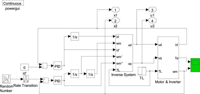
The stator current input is given as 0, the speed input is given as a random quantity with amplitude ranging from 40 rad/s to 140 rad/s, and the sampling system of the PMSM NNIS is shown in Figure 1.

FIGURE 1

FIGURE 1. PMSM inverse system sampling simulation diagram.

Design and Decoupling of BP NNIS for the Permanent Magnet Synchronous Motor

BPNN (Back Propagation Neural Network)

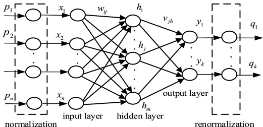
BPNN is an error back propagation feedforward neural network. The structure of the BPNN is shown in Figure 2. The sample input vector p=(p₁, p₂, … , p_n) is normalized to obtain the input layer vector x∈(x₁, x₂, … , x_n)^T. There are m neurons in the hidden layer, and the hidden layer output h=(h₁, h₂, … , h_m)^T is obtained. There are k neurons in the output layer, and the output y=(y₁, y₂, … , y_k)^T of the output layer is obtained. The output is de-normalized to obtain q=(q₁, q₂, … , q_k)^T sample training output. The weight between the input layer and the hidden layer is w_ij, and the threshold is θ_j. The weight between the hidden layer and the output layer is v_jh, and the threshold is τ_h.

FIGURE 2

FIGURE 2. BPNN structure.

The output of neurons in each layer meets the following requirements:

$\{\begin{array}{c}{h}_j=f({\displaystyle \sum _{i=1}^n{w}_{ij}{x}_i}-{\theta }_j)\\ y_h=f({\displaystyle \sum _{j=1}^m{v}_{jh}{h}_j}-{\tau }_h)\end{array}(1)$

Number of Hidden Layer Nodes

There is a relationship among the number of hidden layer neurons J, the input vector dimension n, and the number of partitions M (Yin et al., 2004). Given the other two of them, one of the three parameters can be calculated. In the n-dimensional input space, the maximum number of linearly divisible J hidden layer neurons is

$M(J,n)={\displaystyle \sum _{k=0}^n\left(\begin{array}{c}J\\ k\end{array}\right)}(2)$

Now consider the case that the size of hidden layer nodes is small, when n ≥ J,

$M=\left(\begin{array}{c}J\\ 0\end{array}\right)+\left(\begin{array}{c}J\\ 1\end{array}\right)+\cdots +\left(\begin{array}{c}J\\ J\end{array}\right)=2^J(3)$

It is concluded that the hidden layer with 3 nodes will be able to provide classification, but when J ≥ n, the scale of the input vector must be larger than 3.

According to the above formula, J required to complete the classification as M in the n-dimensional pattern space can be found. This M constitutes the solution of the equation:

$M=1+J+\frac{J(J-1)}{2!}+\cdots +\frac{J(J-1)\cdots (J-n+1)}{n!}J>n(4)$

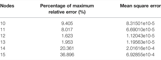
According to the previous section, the BPNN to be trained has 5 inputs and 2 outputs. Set the number of training iterations at net. trainparam. epochs: 2000, net. trainparam. goal: 10e-6 when using MATLAB training. The relationship between prediction error and the number of hidden layer nodes M is shown in Table 1.

TABLE 1

TABLE 1. Prediction error of BPNN with different hidden layer nodes.

The accuracy of neural network prediction decreases first and then increases with the number of nodes increasing. When the number of nodes is 12, the mean square error of prediction is minimum, so the number of nodes in the hidden layer is determined to be 12.

Hidden Layers of the Back Propagation Neural Network

According to Kolmoagorov’s theorem (the representation theorem for continuous functions), given a continuous function:

$\mathrm{\Phi }:E^m\to R^n,\mathrm{\Phi }\left(X\right)=Y(5)$

E^m is a unit cube, then Ф can be precisely realized by a three-layer neural network (Zhao and Wang, 2022a), the first layer of the neural network has 5 processing units, the middle layer has 12 processing units, and the third layer has 2 processing units. The continuity theorem guarantees that any continuous function and mapping can be implemented by a three-layer neural network (Ting, 2017).

When using the single-layer hidden layer BPNN for training, the optimal number of hidden layer nodes is determined to be 12 (Zhao and Wang, 2022a). Now consider using the multi-layer hidden layer, and the prediction error of single-layer and dual-layer BPNN is shown in Table 2.

TABLE 2

TABLE 2. Prediction error of BPNN with different hidden layer nodes.

Compared with the single hidden layer, the multi-hidden layer has stronger generalization ability and higher prediction accuracy, but the training time is longer. When choosing the number of hidden layers, both network precision and training time should be considered. When the network precision meets the requirement, the single hidden layer can be selected to speed up the process (Li et al., 2021a). The comparative analysis not only verifies the reliability of the continuity theorem but also determines the use of the single hidden layer in training.

Back Propagation Neural Network Transfer Function

The transfer function is used to calculate the output of the hidden layer and the output layer, and logsig (S-shaped transfer function) is available:

$f\left(x\right)=\frac{1}{1+e^{-\alpha x_i}}(6)$

tansig (hyperbolic tangent S transfer function):

$f\left(x_i\right)=\frac{1-e^{-\alpha x_i}}{1+e^{-\alpha x_i}}(7)$

purelin (linear transfer function):

$f\left(x_i\right)=x_i(8)$

The default settings tansig and purelin are used for offline training using MATLAB/Simulink as shown earlier. After repeated comparison of different transfer functions, the prediction accuracy is greatly improved when tansig and tansig are used for the transfer functions of the hidden layer and output layer. The prediction errors of the BPNN with different activation functions are shown in Table 3.

TABLE 3

TABLE 3. Prediction error of BPNN with different activation functions.

Therefore, the BPNN is used to select the hyperbolic tangent S transfer function for function fitting approximation (Yin et al., 2004).

The Optimized Back Propagation Neural Network Module Is Generated

Repeated training is needed to determine the optimal parameters of the BPNN, and the neural network module generated by training is used to replace the inverse system for offline decoupling simulation of the BP NNIS of the PMSM (Yin et al., 2004; Pang et al., 2020). The main parameters of the program to generate BPNN are as follows:

net = newff (miN•max (pn) [122], {“tansig”, “tansig”}, “trainlm”, “learngdm”); net. trainPar.epochs = 2000; net. trainPar.show = 10; net. trainPar.goal = 10e-6; net. trainPar.min_grad = 1e-15;

net.trainPar.mu_dec = 0.1; net. trainPar.mu_inc = 7; net. trainPar.goal = 0.04; net. trainPar.lr = 0.5;

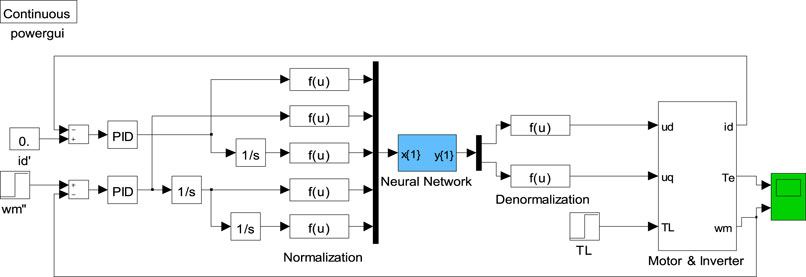
The PMSM decoupling control system based on the BP NNIS can be constructed by replacing the inverse system module with the generated BPNN module and adding normalization and inverse normalization modules before and after the neural network module, as shown in Figure 3.

FIGURE 3

FIGURE 3. NNIS of PMSM decoupling control system.

The parameter setting of PI and PD regulator of BP NNIS is shown in Table 4.

TABLE 4

TABLE 4. PID parameters of BP NNIS.

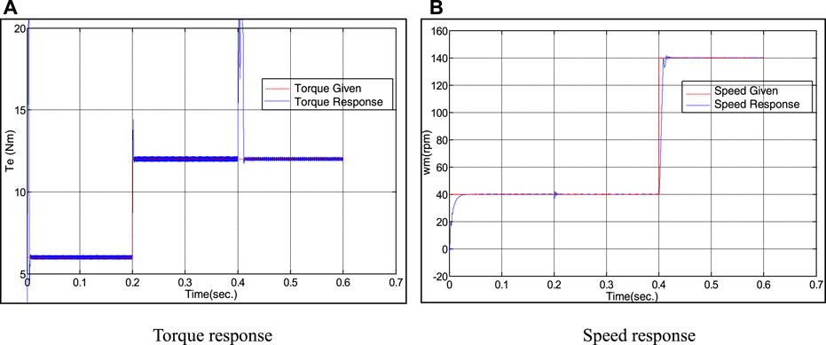
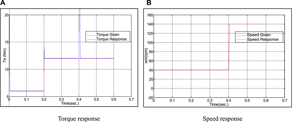
At 0–0.2 s, the given load torque TL is 6 N m, and at 0.4 s, the load torque mutates to 12 N m; at 0–0.4 s, the given rotor speed ωr is 40 rad/s, in 0.4 s, ωr changes to 140 rad/s. Torque and speed response curves under inverse control mode are shown in Figure 4, and Figure 5 shows the torque and speed response curves of the inverse system based on the BPNN under the same conditions (Zhang, 2010).

FIGURE 4

FIGURE 4. Response curve of inverse system decoupling control.

FIGURE 5

FIGURE 5. Response curve of BPNN inverse system decoupling control.

Comparing Figure 4 and Figure 5, it can be found that when the set load torque changes suddenly, both controls can maintain the stability of load speed, but the inverse system control method has long torque response time and large peak value, and the peak value of torque reaches 17 N m. The overshoot is 41%, while the torque response time of BP NNIS is short and the peak value is small, and the overshoot is only 16%. When the set speed changes suddenly, the speed response of the two control modes is relatively fast, and there is basically no overshoot. However, in the inverse system control mode, the torque fluctuation is large and the adjustment time is long, while in the BP NNIS, the torque fluctuation is small and the recovery time is short.

In the test, the speed is kept at 90 rad/s, and the load has periodic step change between 6 N m and 12 N m rated load torque. The response curve of speed and torque under inverse control mode is shown in Figure 6. Figure 7 shows the speed and torque response curves of the inverse system based on the BPNN under the same conditions.

FIGURE 6

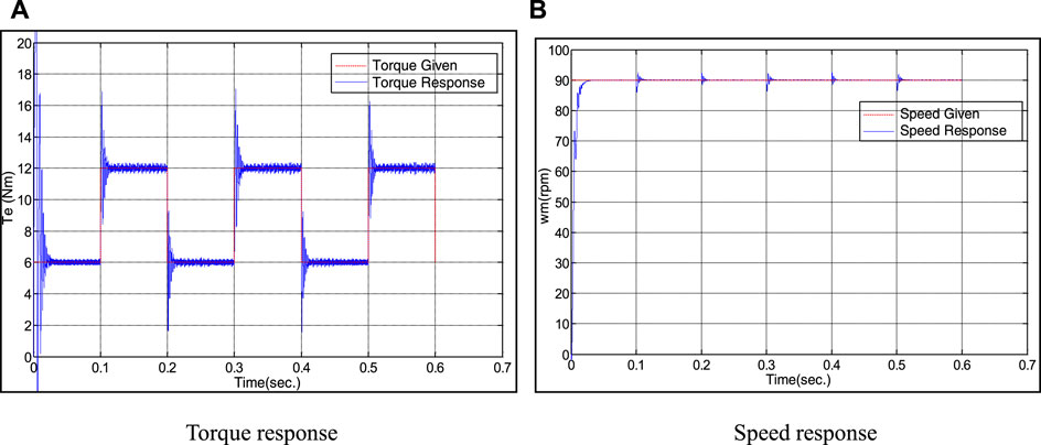
FIGURE 6. Response curve of BPNN inverse system decoupling control when torque changes periodically.

FIGURE 7

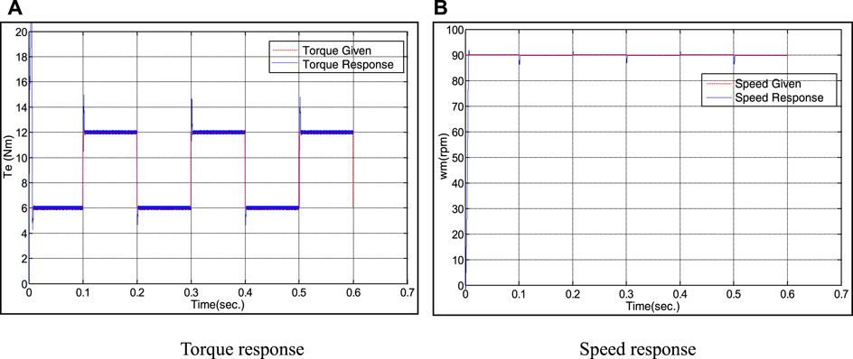
FIGURE 7. Response curve of BPNN inverse system decoupling control when torque changes periodically.

Comparing Figure 6 and Figure 7, it is not difficult to find that when the rated load torque changes periodically, the two control modes can maintain the speed stability, but under the inverse system control mode based on BPNN, the torque response overshoot is smaller and the adjustment time is shorter.

Inverse System Design and Decoupling of Radial Basis Function Neural Network for Permanent Magnet Synchronous Motor

Radial Basis Function Neural Network

RBFNN as a feedforward network can approximate analytic nonlinear relations with arbitrary accuracy (Wang et al., 2022; Yang et al., 2020). It is a powerful tool to deal with complex nonlinear, uncertain, and coupling problems in MIMO systems. Now a PMSM decoupling control system based on the RBF NNIS is established (Zhao and Wang, 2022b), which makes the system have good dynamic and static characteristics.

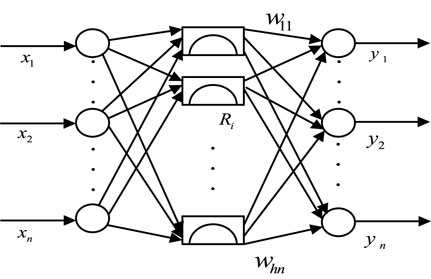
The RBF neural model is shown in Figure 8.

FIGURE 8

FIGURE 8. RBF neural model. RBFNN structure as shown in Figure 9.

FIGURE 9

FIGURE 9. RBF neural network.

Before using the RBFNN, it is necessary to determine the number of hidden layer neurons, the center of transfer function, expansion constant, and a set of corresponding weights.

Structure of the Radial Basis Function Neural Network

The design methods of the RBFNN can be divided into two categories (Li et al., 2020; Li et al., 2021b; Huang et al., 2022).

1) The function center is randomly selected from the sample data and the center is fixed. After the RBF center is determined, the output of hidden layer is known (Chen, 2021).

Gaussian function is selected as radial basis function, so the transfer function of radial basis function neural network can be expressed as

$R(X-c_i)=\exp (-\frac{M}{d_m^2}||X-c_i{||}^2)(9)$

In the formula, M is the number of neurons in the hidden layer; d_m is the maximum distance between the selected centers. In this case, the mean square deviation of Gaussian RBF is fixed as

$\sigma =\frac{d_m}{\sqrt{2M}}(10)$

The connection weight of the network can be directly calculated by the previous formula:

$W=R^{+}d(11)$

In the formula, d is the desired response vector. R⁺ is the pseudo inverse of matrix R, and R is determined by

$R=\left\{r_{ji}\right\}(12)$

$g_{ji}=\exp (-\frac{M}{d_m^2}||X_j-c_i{||}^2)(13)$

In the formula, X_j is the data quantity of the jth input sample, and the singular value decomposition method can be used to calculate the pseudo inverse of the matrix. This method corresponds to the MATLAB/newrb construction method.

2) In the dynamic adjustment method of function center, the center of RBF is moved, and its position is determined by self-organizing learning, while the linear weight of the output layer is calculated by supervised learning rules. The purpose of learning is to have the center of RBF located in the important area of input space. The specific steps are as follows:

1) Initialize the cluster center c_i. Generally, M samples are selected from the input sample X_i as the clustering center.

2) The input samples are grouped according to the nearest neighbor rule (Zuo et al., 2014); that is, M samples in Xi are assigned to the input sample cluster set θ_i with center c_i, that is, X_j∈θ_i, and meet

$d_i=\min \left|\right|X_j-c_i\left|\right|(14)$

where d_i represents the minimum Euclidean distance.

3) Calculate the mean value of samples in θ_i (i.e., clustering center c_i)

$c_i=\frac{1}{M_i}{\displaystyle \sum _{x_j\in {\theta }_j}{X}_j}(15)$

where M_i is the number of input samples in θ_i. Calculate according to the aforementioned steps until the distribution of cluster center no longer changes. After the center of RBF is determined, if RBF is a Gaussian function, its mean square deviation σ can be calculated by Eq. 18. The output of the hidden layer can then be calculated. This method corresponds to the MATLAB/newrbe construction method.

Newrb and newrbe were, respectively, used to establish two kinds of RBFNNs. The error of the sum of squares was set as 10e-4 pairs of neurons. By comparing the sum of square error, the structure prediction error of different RBFNNs is shown in Table 5.

TABLE 5

TABLE 5. Prediction error of different RBFNN structures.

By comparison, it is concluded that newrbe can only be stopped when the number of neurons reaches the number of training samples. Although the required error precision is reached, the running time is too long. On the contrary, newrb can use fewer neurons to achieve the error precision, and the running time is shorter.

The Spread of the Radial Basis Function Neural Network

When applying the newrbe function to the design of the radial basis function neural network, the spread needs to cover as many input intervals as possible (Li et al., 2019b; Yang et al., 2019), so it needs to be set as large as possible. However, too large spread will lead to the difficulty of numerical calculation, and the corresponding regions cross too much, which will reduce the accuracy. Reasonable selection of spread values has great influence on the prediction accuracy of the RBFNN. Newrb is used to construct the RBFNN and spread is set as different values for comparison (Wang and Xu, 2012; Pang et al., 2020). The prediction errors of different RBF spreads are shown in Table 6.

TABLE 6

TABLE 6. Prediction error of different RBF spread.

Generating Optimized Back Propagation Neural Network Module

In addition, the display interval was set as 1, the maximum number of neurons was set as 600, and the neural network module generated by training was used to replace the inverse system for the decoupling offline simulation of the inverse system of the RBFNN of the PMSM. The main parameters of the program to generate the RBFNN (Zuo et al., 2014) are as follows:

goal = 0.0001; spread = 1; MN = 600; DF = 1;

net = newrb (pn, tn, goal, spread, MN, DF);

By replacing the inverse system module with the generated RBFNN module, and adding the normalized and anti-normalized modules in the front and back to the neural network module, a PMSM decoupling control system based on the NNIS can be constructed, as shown in Figure 3.

The parameter setting of PI and PD regulator of RBF NNIS is shown in Table 7.

1) Static decoupling experiment under the same conditions as section 3:

TABLE 7

TABLE 7. PID parameters of RBF NNIS.

Figure 10 shows the torque and speed response curves under the RBF NNIS control mode under the same conditions.

FIGURE 10

FIGURE 10. Response curve of RBFNN inverse system decoupling control.

Comparing Figure 10A with Figure 5A, it can be found that when the speed remains unchanged and the torque changes suddenly, the control mode based on the RBF NNIS has faster response speed and shorter system stability time than BPNN. When the speed changes suddenly, the RBF NNIS also has a faster response speed.

2) Dynamic decoupling experiment against load disturbance under the same conditions as in Section 3:

Figure 11 shows the torque and speed response curves under the RBF NNIS control mode under the same conditions.

FIGURE 11

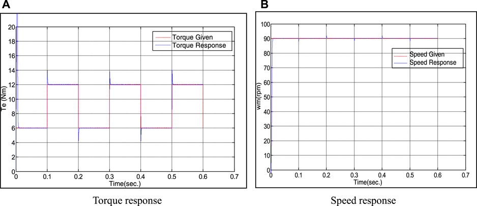
FIGURE 11. Response curve of RBFNN inverse system decoupling control when torque changes periodically.

Comparing Figure 7A with Figure 11A, it can be found that when the set speed remains unchanged and the torque changes step periodically, the control method based on the RBF NNIS has faster response speed, smaller overshoot, and more stable torque in a steady state than BPNN torque regulation. Comparing Figure 11B with Figure 7B, it can be found that when the torque changes suddenly, the speed of the RBF NNIS is also more stable.

Decoupling Performance Analysis

The static decoupling test can verify the static decoupling performance of the system, that is, the stability of one variable when the other variable changes. It can be seen from Figure 5 that the inverse decoupling control system based on the RBFNN has a very small overshoot, basically no oscillation, and the fastest response time when the speed and torque change.

The anti-load disturbance experiment can verify the dynamic decoupling performance of the system, and the dynamic decoupling performance is an important criterion for evaluating the advantages and disadvantages of the decoupling system. As can be seen from Figure 7, the inverse decoupling control system based on the RBFNN responds rapidly and is basically synchronized with the given load. The speed response under the control mode of the inverse system decoupling control system based on the RBFNN has no overshoot, the oscillation amplitude is very small, and the stability value is quickly restored. The speed response of the inverse system decoupling control system based on the BPNN has overshoot and large oscillation amplitude. Under the control mode of the inverse system decoupling control system (Bu et al., 2018), speed has a long-time jitter, and the recovery to the stable value is slow.

Conclusion

After verification and comparative analysis, it can be confirmed that the PMSM based on the RBF NNIS control mode has excellent static decoupling characteristics and better dynamic decoupling control performance. The simulation research based on RBF NNIS decoupling control has good robustness and stability compared with the other two decoupling controls. This is an optimized NNIS PMSM decoupling control system, which has a certain application value.

Data Availability Statement

The original contributions presented in the study are included in the article/Supplementary Material. Further inquiries can be directed to the corresponding author.

Author Contributions

GD-W is responsible for the MATLAB modeling of PMSM. QZ-Q, ZW, and KZ-W are responsible for theoretical derivation. LY is responsible for neural network inverse system simulation.

Funding

This work was supported by the National Defense Pre-Research Foundation of China (1126170104A, 1126180204B, 1126190508A, and 1126190508A).

Conflict of Interest

The authors declare that the research was conducted in the absence of any commercial or financial relationships that could be construed as a potential conflict of interest.

Publisher’s Note

All claims expressed in this article are solely those of the authors and do not necessarily represent those of their affiliated organizations, or those of the publisher, the editors, and the reviewers. Any product that may be evaluated in this article, or claim that may be made by its manufacturer, is not guaranteed or endorsed by the publisher.

Acknowledgments

All data included in this study are available upon request by contact with the corresponding author.

References

Bu, W., Chen, Y., and Zu, C. (2019). Stator Flux Orientation Inverse System Decoupling Control Strategy of Bearingless Inductionmotor Considering Stator Current Dynamics[J]. IEEJ Trans. Electr. Electron. Eng. 14 (4), 22847. doi:10.1002/tee.22847

CrossRef Full Text | Google Scholar

Bu, W., He, F., Li, Z., Zhang, H., and Shi, J. (2018). Neural Network Inverse System Decoupling Control Strategy of BLIM Considering Stator Current Dynamics. London: Transactions of the Institute of Measurement and Control.

Google Scholar

Bu, W., Li, B., He, F., and Li, J. (2019). Inverse System Decoupling Sliding Mode Control Strategy of BLIM Considering Current Dynamics. Int. J. Appl. Electromagn. Mech. doi:10.3233/jae-180094

CrossRef Full Text | Google Scholar

Bu, W., and Li, Z. (2019). LS-SVM Inverse System Decoupling Control Strategy of a Bearingless Induction Motor Considering Stator Current Dynamics[J]. IEEE Access (99), 1. doi:10.1109/ACCESS.2019.2939258

CrossRef Full Text | Google Scholar

Bu, W., Li, Z., and Wang, X. (2015). “A Control Method of Bearingless Induction Motor Based on Neural Network[C],” in IEEE International Conference on Information & Automation, Lijiang, August 8–10, 2015 (IEEE).

Google Scholar

Chen, Y. (2021). College English Teaching Quality Evaluation System Based on Information Fusion and Optimized RBF Neural Network Decision Algorithm. J. Sensors. doi:10.1155/2021/6178569

CrossRef Full Text | Google Scholar

Huang, B., Li, Y., Zhan, F., Sun, Q., and Zhang, H. (2022). A Distributed Robust Economic Dispatch Strategy for Integrated Energy System Considering Cyber-Attacks. IEEE Trans. Ind. Inf. 18, 880–890. doi:10.1109/TII.2021.3077509

CrossRef Full Text | Google Scholar

Jie, H., Xu, H., and Zheng, G. (2020). Adaptive Decoupling Control Using Radial Basis Function Neural Network for PMSM Considering Uncertain and Time-Varying Parameters[J]. IEEE Access (99), 1. doi:10.1109/ACCESS.2020.2993648

CrossRef Full Text | Google Scholar

Li, B., Quan, Z., Bei, S., Zhang, L., and Mao, H. (2021). An Estimation Algorithm for Tire Wear Using Intelligent Tire Concept. Proc. Institution Mech. Eng. Part D J. Automob. Eng. doi:10.1177/0954407021999483

CrossRef Full Text | Google Scholar

Li, S., Won, H., and Fu, X. (2019). Neural-Network Vector Controller for Permanent-Magnet Synchronous Motor Drives: Simulated and Hardware-Validated Results[J]. IEEE Trans. Cybern. (99), 1. doi:10.1109/TCYB.2019.2897653

CrossRef Full Text | Google Scholar

Li, Y., Gao, D. W., Gao, W., Zhang, H., and Zhou, J. (2021). A Distributed Double-Newton Descent Algorithm for Cooperative Energy Management of Multiple Energy Bodies in Energy Internet. IEEE Trans. Ind. Inf. 17 (9), 5993–6003. doi:10.1109/tii.2020.3029974

CrossRef Full Text | Google Scholar

Li, Y., Gao, D. W., Gao, W., Zhang, H., and Zhou, J. (2020). Double-Mode Energy Management for Multi-Energy System via Distributed Dynamic Event-Triggered Newton-Raphson Algorithm. IEEE Trans. Smart Grid. 11 (6), 5339–5356. doi:10.1109/tsg.2020.3005179

CrossRef Full Text | Google Scholar

Li, Y., Zhang, H., and Liang, X. (2019). Event-triggered Based Distributed Cooperative Energy Management for Multienergy Systems. IEEE Trans. Ind. Inf. 15 (14), 2008–2022. doi:10.1109/tii.2018.2862436

CrossRef Full Text | Google Scholar

Pang, Z., Wang, T., Liu, S., Wang, Z., and Gong, L. (2020). Kinematics Analysis of 7-DOF Upper Limb Rehabilitation Robot Based on BP Neural Network,” in IEEE 9th Data Driven Control and Learning Systems Conference (DDCLS), Liuzhou, November 20–22, 2020 (IEEE). doi:10.1109/ddcls49620.2020.9275138

CrossRef Full Text | Google Scholar

Sun, X., Long, C., and Jiang, H. (2016). High-Performance Control for a Bearingless Permanent-Magnet Synchronous Motor Using Neural Network Inverse Scheme Plus Internal Model Controllers[J]. IEEE Trans. Industrial Electron. 63 (6), 1. doi:10.1109/tie.2016.2530040

CrossRef Full Text | Google Scholar

Ting, L. (2017). “An Empirical Study on China's Early Warning of Financial Risks under the New Normal,” in 2017 4th International Conference on Industrial Economics System and Industrial Security Engineering, Kyoto, July 24–27, 2017 (IEIS).

Google Scholar

Wang, H. F., and Xu, X. A. (2012). Applying RBF Neural Networks and Genetic Algorithms to Nonlinear System Optimization. Adv. Mater. Res 16 (6), 115–118. doi:10.4028/www.scientific.net/amr.605-607.2457

CrossRef Full Text | Google Scholar

Wang, X., Gao, D. W., Yan, J. W., Gao, W., Muljadi, E., and Gevorgian, V. (2018). Implementations and Evaluations of Wind Turbine Inertial Controls with FAST and Digital Real-Time Simulations. IEEE Trans. Energy Convers. 33 (4), 1805–1814. doi:10.1109/tec.2018.2849022

CrossRef Full Text | Google Scholar

Wang, X., Zhao, T., and Parisio, A. (2022). Frequency Regulation and Congestion Management by Virtual Storage Plants. Sustain. Energy, Grids Netw. 29 (1), 100586. doi:10.1016/j.segan.2021.100586

CrossRef Full Text | Google Scholar

Xie, M., and Xie, L. (2020). Decoupling Control of Permanent Magnet Synchronous Motor with Support Vector Regression Inverse System Method. IEEE Access 8, 212687–212698. doi:10.1109/access.2020.3039053

CrossRef Full Text | Google Scholar

Yang, T., George, J., Qin, J., Yi, X., and Wu, J. (2020). Distributed Least Squares Solver for Network Linear Equations. Automatica 113.

CrossRef Full Text | Google Scholar

Yin, F. L., Wang, J., and, , and Guo, H. (2004). Advances in Neural Networks - ISNN 2004. Berlin: Springer Science and Business Media LLC

Google Scholar

Yang, T., Yi, X., Wu, J., Yuan, Y., Wu, D., Meng, Z., et al. (2019). A Survey of Distributed Optimization. Annu. Rev. Control 47, 278–305. doi:10.1016/j.arcontrol.2019.05.006

CrossRef Full Text | Google Scholar

Zhang, D. (2010). Energy-Saving Control Based on Neural Network Inverse Decoupling for Asynchronous Motors,” in Asia-Pacific Power and Energy Engineering Conference.03.

Google Scholar

Zhao, W., and Wang, C. (2022). Decoupling Control of Nonlinear Inverse System for Chassis-By-Wire System. Berlin: Springer Science and Business Media LLC.

Google Scholar

Zhao, W., and Wang, C. (2022). Nonlinear Control Technology of Vehicle Chassis-By-Wire System. Berlin: Springer Science and Business Media LLC.

Google Scholar

Zuo, G. L., Niu, F. L., Cheng, Y., and Zhang, Y. X. (2014). Study on the Fault Diagnosis of Gear Pump Based on RBF Neural Network. Applied Mechanics and Materials. doi:10.4028/www.scientific.net/amm.556-562.2957

CrossRef Full Text | Google Scholar