A Robust Scheduling Methodology for Integrated Electric-Gas System Considering Dynamics of Natural Gas Pipeline and Blending Hydrogen

As smart grid develops and renewables advance, challenges caused by uncertainties of renewables have been seriously threatening the energy system’s safe operation. Nowadays, the integrated electric-gas system (IEGS) plays a significant role in promoting the flexibility of modern grid owing to its great characteristic in accommodating renewable energy and coping with fluctuation and uncertainty of the system. And hydrogen, as an emerging and clean energy carrier, can further enhance the energy coupling of the IEGS and promote carbon neutralization with the development of power-to-hydrogen (P2H) technology and technology of blending hydrogen in the natural gas system. Dealing with the uncertainty of renewables, a robust schedule optimization model for the integrated electric and gas systems with blending hydrogen (IEGSH) considering the dynamics of gas is proposed and the iterative solving method based on column-and-constraint generation (C&CG) algorithm is implemented to solve the problem. Case studies on the IEGSH consisting of IEEE 39-bus power system and 27-node natural gas system validate the effectiveness of the dynamic energy flow model in depicting the transient process of gas transmission. The effectiveness of the proposed robust day-ahead scheduling model in dealing with the intra-day uncertainty of wind power is also verified. Additionally, the carbon emission reduction resulting from the blending of hydrogen is evaluated.

1 Introduction

The energy dilemma and environmental pollution problems motivate the policy and public awareness on fossil resource depletion and renewable energy resource development (Liu et al., 2019). As smart grid and other energy systems develop, much effort has been made to advance the renewable energy system mitigating climate change and realizing sustainable development (Kim et al., 2021). The share of electric power supplied by renewables is increasing up to 57% of the electric load in 2050, according to the forecasting of the International Energy Agency (IEA) (Brouwer et al., 2014). However, the intermittency of renewables, such as wind and photovoltaic power generation, requires more flexibility of the energy system (Erdiwansyah et al., 2021). The integration of multiple energy systems, including electric system, natural gas system, heating system, cooling system, and so on, is capable of promoting the efficiency and flexibility of energy utilization (Zhu et al., 2021).

Among various energy systems, the electric system and natural gas system are the most common choices for large-scale transmission of energy (Fang et al., 2018). The gas-fired unit (GFU) can connect the two systems, which can respond quickly to the output power fluctuation of renewables, such as wind plant, photovoltaic power generation, and so on (Shu et al., 2019). And the operation of the electric system and natural gas system is increasingly coupled owing to the development of the power-to-gas (P2G) technologies, which can transfer surplus renewables into methane and the natural gas can act as energy storage since gas pipeline is of enormous potential for energy storage. The integration of the two systems can promote the flexibility of the energy system and the accommodation of volatile renewables.

With the development of utilization and storage technologies of hydrogen, the combination of power-to-hydrogen (P2H) technology and renewables generation technology is regarded as a promising way to accommodate the surplus renewable energy and moderate fluctuations (Ban et al., 2017). Meanwhile, the hydrogen is clean with high energy density and can be utilized in many fields without carbon emission, which can act as an ideal energy storage carrier (Kavadias et al., 2022). The potential maximum demand of hydrogen is up to 158 Mt in 2030 and 568 Mt in 2050 according to the results of forecasting in (Yusaf et al., 2022). And coupling the hydrogen with existent energy system can help the carbon emission reduction. In (Hu et al., 2020), a model of power-to-heat and hydrogen (P2HH) is proposed and an optimal control framework of a microgrid considering the P2HH is established. The result shows that the P2HH can help improve the efficiency of the overall system. In (Li et al., 2019), the simplified P2HH model is used in the dispatch problem coordinated with active distribution networks and district heating networks. Blending hydrogen into natural gas pipeline networks as an emerging technology can deal with the problem that the storage cost for hydrogen is too high and make it possible for mass storage of hydrogen (Zhou et al., 2022). In (Mehra et al., 2017; Yan et al., 2018), the adaptability of GFU to natural gas blended hydrogen is reviewed and they point out that most existing GFU can adapt up to 30% or even a higher proportion of blended hydrogen natural gas technically. However, few researches are focusing on the operation optimization of integrated electric and gas systems with blending hydrogen (IEGSH).

As for the integrated electric and gas systems (IEGS), many studies have been carried out focusing on its operation optimization problem and establishing the mathematical model. In (Martinez-Mares and Fuerte-Esquivel.,2012), the steady-state model of IEGS is proposed and analyzed considering the influence of temperature of the natural gas system. In (Zeng et al., 2016), the steady-state energy flow of the natural gas system is established and combined with the electric energy flow and the Newton-Raphson method is adopted to solve the problem. In (Sahin et al., 2012; Li et al., 2008; Liu et al., 2009), the steady-state energy flow equation is also adopted and the operation optimization of IEGS is studied focusing on the safety and risk-related problems. The above researches are all based on the steady-state energy flow description methods, in which the difference between the velocity of energy flow in the electric system and natural gas system is neglected. However, the operation of the two systems belongs to different time scales and the transient process of the gas in the pipeline is supposed to be considered to describe the transmission process of the gas pipeline more precisely and guarantee operation safety.

In order to reflect the dynamic energy flow of the gas movement along the pipes and the different time constant of the natural gas system from that of an electric system, relevant researches are conducted in recent years (Jiang et al., 2018; Zheng et al., 2017). In (Liu et al., 2011), the transient characteristics of natural gas flow are depicted and the implicit finite difference method is applied to simplify the transient energy flow equations. However, the independent optimization of the natural gas system and the electric system is adopted to achieve the coordinated optimization of the IEGS by solving iteratively. In (Hang et al., 2017), the linear programming formulation for IEGS considering the transient gas energy flow has been proposed and solved by using the approximated dynamic programming algorithm. The result of the IEGS coordinated optimization considering the dynamic characteristic of the gas pipeline has been shown in these works, but the effect of P2G unit coupling into the natural gas system is not taken into consideration. Meanwhile, the effect of volatile renewable energy in the IEGS is also not considered.

Relevant problems resulting from the uncertainty in the energy system have also drawn much interest in the past decades. In (Bai et al., 2017), a robust scheduling model against wind power uncertainty under the random pipeline and transmission N-1 contingencies is proposed. In (He et al., 2017), a robust optimization scheduling model for IEGS is established to optimize the operation of the two energy systems considering key uncertainties in the electric system, while the model is solving the electric system sub-problem and natural gas system sub-problem iteratively. In (Zhang et al., 2016), a stochastic day-ahead schedule optimization problem of IEGS is studied and it adopts the Monte Carlo simulation method to generate multiple scenarios to represent the uncertainties of the considered integrated systems. In (Li et al., 2018; Li et al., 2021), the scenario generation method is applied to depict the uncertainty of the IEGS and the scenario reduction method is also adopted to eliminate scenarios with lower probabilities. In (Zhang et al., 2020), the ambiguity set of wind power based on the confidence bands of its probability density function is formulated to describe the uncertainty of wind power. In (Odetayo et al., 2018; Ding et al., 2018), stochastic programming is applied to deal with the uncertainties of renewables. The stochastic programming and scenario generation method are supposed to be based on the probability density distribution of uncertain parameters, which is hard to be depicted precisely.

To sum up, the IEGS can promote the efficiency of energy utilization and the flexibility of the IEGS operation. And hydrogen plays a more and more significant role in the energy supply owing to its superior characteristic and can act as one of the best options for large-scale energy storage. There have been a lot of researches carried out focusing on the operation optimization problem of IEGS and the combining P2H unit with the traditional energy system. However, the existing researches mostly apply the steady-state flow equation to depict the operation in natural gas system, which cannot reflect the real dynamic process of gas in the pipeline. Meanwhile, previous studies mainly focus on the coordinating operation of IEGS without considering the blending of hydrogen and deal with the uncertainties of IEGS by scenario-based method and stochastic programming.

Focusing on the scheduling optimization problem of the IEGSH, this paper proposes a robust scheduling framework considering the uncertainty of the wind power. And the dynamic energy flow equation for the blended gas is derived, while the blending of hydrogen in the natural gas system is considered. The main contributions of this work are as follows:

1) Considering the blending of hydrogen in the natural gas system, a mass flow rate calculation model for blended gas based on the constant volume ratio assumption is derived.

2) The energy flow model of the natural gas system considering the hydrogen blending and the dynamic characteristic is proposed to describe the dynamic operation process of the gas pipeline with more accuracy.

3) To promise better economy and robustness, a day-ahead schedule optimization model for the IEGSH is proposed and the uncertainty of the wind power is taken into consideration. And an iterative solving method based on the column-and-constraint generation (C&CG) algorithm is proposed to solve the problem.

The rest of this paper is structured as follows. In Section 2, the model of dynamic energy flow in the natural gas system considering the hydrogen blending is established. In Section 3, the schedule optimization framework without considering the uncertainty is presented. In Section 4, the robust schedule optimization model is established and the solving algorithm is also introduced. In Section 5, the case study is presented. And conclusions of this work are drawn in Section 6.

2 Energy Flow in the Natural Gas System With Hydrogen Blending

In this section, the calculating formulation of the mass flow rates of the hydrogen and methane at each node of the natural gas system considering the constant blending volume ratio of the hydrogen is firstly derived. And then the model of the natural gas system with hydrogen blending considering the dynamics of the system is established.

2.1 Formulation of the Mass Flow Rates of the Hydrogen and Methane

The volume ratio of the hydrogen blending into the natural gas pipeline is assumed to keep constant in order to guarantee the security and stability of the natural gas system. Based on this assumption, the volume ratio of the hydrogen and the methane can be calculated by the following equation.

$R_V=\frac{V_H}{V_M}(1)$

where $R_V$ represents the volume ratio of the hydrogen and methane; $V_H$ and $V_M$ represent the volume of the hydrogen and methane, respectively.

Given the volume ratio, the mass flow rates of the hydrogen and methane of the natural gas system at each time $t$ can be determined according to the Eqs 2–5 as follows.

$R_V=\frac{V_H\left(t\right)}{V_M\left(t\right)}(2)$

$Q_H\left(t\right)=\frac{{\rho }_H\left(t\right)V_H\left(t\right)}{\mathrm{\Delta }t}(3)$

$Q_M\left(t\right)=\frac{{\rho }_M\left(t\right)V_M\left(t\right)}{\mathrm{\Delta }t}(4)$

$\frac{Q_H\left(t\right)}{Q_M\left(t\right)}=\frac{{\rho }_H\left(t\right)}{{\rho }_M\left(t\right)}{R}_V(5)$

where $V_H\left(t\right)$ and $V_M\left(t\right)$ represent the volume of the hydrogen and methane at time t, respectively; ${\rho }_H\left(t\right)$ and ${\rho }_M\left(t\right)$ represent the density of the hydrogen and methane at time t, respectively; $Q_H\left(t\right)$ and $Q_M\left(t\right)$ represent the mass flow rate of the hydrogen and methane at time t, respectively; and $\Delta t$ represents the time interval.

Then the Eq. 6 can be derived, which describes the relationship between the mass flow rate of the hydrogen and that of the methane.

$\frac{Q_H\left(t\right)}{Q_M\left(t\right)}=\frac{{\rho }_H\left(t\right)}{{\rho }_M\left(t\right)}{R}_V=K\left(t\right)(6)$

where K(t) represents the relationship coefficient between the mass flow rate of the hydrogen and that of the methane.

The mass flow rate of the blended gas is equal to the sum of those of hydrogen and methane. Therefore, the relationships among mass flow rate of hydrogen, methane, and blended gas can be described as Eqs 7, 8, according to Eq. 6.

$Q_H\left(t\right)=\frac{K\left(t\right)}{K\left(t\right)+1}{Q}_b\left(t\right)(7)$

$Q_M\left(t\right)=\frac{1}{K\left(t\right)+1}{Q}_b\left(t\right)(8)$

where $Q_b\left(t\right)$ represents the mass flow rate of the blended gas.

There are various forms of the equation of gas state to link the pressure, temperature, and density. Taking the ideal gas law, indicating $PV=nRT$, for example, it only works at less than 1 MPa and 20°C. In this paper, a simple form, i.e. Eq. 9, of the equation of gas state is adopted to describe the relationship between the pressure and density of the gas by the link of the sound speed.

$P=c^2\rho (9)$

And the relationship between the gas pressure and density can be depicted as Eq. 10.

$P_{(\cdot )}\left(t\right)=c^2{\rho }_{(\cdot )}\left(t\right)(10)$

where subscript $(\cdot )$ can represents hydrogen and methane.

When the gas is at the standard state, the state equation can be described as Eq. 11.

$P_{(\cdot )}^{\ast }\left(t\right)=c^2{\rho }_{(\cdot )}^{\ast }\left(t\right)(11)$

where superscript ∗ represents that the gas is at the standard state.

According to Eqs 10, 11, the relationship coefficient K(t) can be determined by the following Eq. 12, which is constant, denoted as K.

$K\left(t\right)=\frac{{\rho }_H^{\ast }\left(t\right)}{{\rho }_M^{\ast }\left(t\right)}{R}_V^2=K(12)$

2.2 Dynamic Energy Flow of the Natural Gas System With Blending Hydrogen

The velocity of the energy flow in the natural gas system is exactly different from that in the power system and the dynamics of the gas in the gas pipeline should be taken into consideration to describe the operation process of the natural gas system accurately and ensure the safety of the system. And the dynamic process can be depicted by using three major equations: momentum equation, material balance equation, and gas state equation. The gas state equation adopted in this work is introduced in Section 2.1, which is described as Eq. 9.

The momentum equation and material balance equation take the forms of Eqs 13, 14, respectively.

$\frac{\partial \left(\rho v\right)}{\partial t}+\frac{\partial \left(\rho v^2\right)}{\partial x}+\frac{\partial P}{\partial x}+\mathrm{g}\left(\rho -{\rho }_{\theta }\right)\sin \theta +\frac{\lambda }{D}\frac{v^2}{2}\rho =0(13)$

$\frac{\partial \rho }{\partial t}+\frac{\partial \left(\rho v\right)}{\partial x}=0(14)$

where $P$ and $v$ represent the pressure and flow velocity of the mixed gas in the natural gas pipeline, respectively; $\rho$ and ${\rho }_{\theta }$ represent the density of the blended gas in the position parallel to the horizontal plane and with an angle $\theta$ to the horizontal plane, respectively; $\lambda$ represents the friction coefficient between gas and pipeline; $D$ represents the inner diameter of the pipeline; $g$ represents the gravitational acceleration; $x$ and $t$ represent the temporal and spatial distance, respectively.

As for Eq. 13, the first, second, third, and fourth term describes the acceleration, convective, hydrostatic, and altitudinal effects of the gas in the pipeline, respectively. And the fifth term describes the second-order deviation of the gas pipeline. It is very complex, and some assumptions are adopted to simplify the dynamic equations. Firstly, the gas transmission in the pipeline is assumed to be isothermal so that the gas temperature variation is neglected and the sound speed c also becomes constant. The second assumption is that the altitude of the pipeline remains unchanged so that $\theta =0$. Therefore, the fourth term in Eq. 13 is equal to 0. Owing to that the convective term only consists when the velocity of the gas approaching to sound speed, the corresponding term can also be neglected. Based on the above assumptions, the momentum equation of the blended gas can be transferred into the form of Eq. 15.

$\frac{\partial \left(\rho v\right)}{\partial t}+\frac{\partial P}{\partial x}+\frac{\lambda }{D}\frac{v^2}{2}\rho =0(15)$

2.3 Linearized Dynamic Energy Flow Model

The dynamic energy flow equations are derived based on some assumptions in Section 2.2, i.e., Eqs 9, 13, 15 which are partial differential equations. Describing the dynamic energy flow in the gas pipeline by using these equations is complicated and they are hard to be implemented when it comes to the operation optimization problem of the real system. In this work, linearization and some simplifications are adopted to turn the partial differential equations into their corresponding differential forms.

Firstly, the mass flow rate of the blended gas, denoted as Q, is introduced and the relationship between mass flow rate and flow velocity of the mixed gas is described as Eq. 16.

$Q=\rho vS(16)$

where Q represents the mass flow rate of the mixed gas, and S indicates the cross-sectional area of the pipeline.

Furthermore, as for the quadratic term of flow velocity in Eq. 15, the average flow velocity is introduced to make the term linearized. Further, the relationship between the density and pressure of the mixed gas, i.e. Eq. 9, can be applied to simplify Eqs 14, 15. Then the momentum equation and material balance equation become

$\frac{\partial Q}{S\partial t}+\frac{\partial P}{\partial x}+\frac{\lambda \overline{v}}{2DS}Q=0(17)$

$\frac{\partial P}{c^2\partial t}+\frac{\partial Q}{S\partial x}=0(18)$

where $\overline{v}$ represents the average flow velocity of mixed gas.

The dynamic energy flow equations with partial differential form are differential linearized based on the Wendroff difference method. The Wendroff difference form is shown as Eq. 19 and its scheme is shown in Figure 1.

$\begin{array}{c}\frac{\partial J(x,t)}{\partial t}\approx \frac{1}{2}\left(\frac{J_{i+1,t+1}-J_{i+1,t}}{\mathrm{\Delta }t}+\frac{J_{i,t+1}-J_{i,t}}{\mathrm{\Delta }t}\right)\\ \frac{\partial J(x,t)}{\partial x}\approx \frac{1}{2}\left(\frac{J_{i+1,t+1}-J_{i,t+1}}{\mathrm{\Delta }x}+\frac{J_{i+1,t}-J_{i,t}}{\mathrm{\Delta }x}\right)\\ J(x,t)\approx \frac{1}{4}\left(J_{i+1,t+1}+J_{i+1,t}+J_{i,t+1}+J_{i,t}\right)\end{array}(19)$

where $J(x,t)$ indicates a function of the space and time at the same time; $\Delta x$ and $\Delta t$ represent the spatial and temporal step, respectively; $J_{i,t}$ represents the differential value of $J(x,t)$ at node $i$ and time $t$.

FIGURE 1

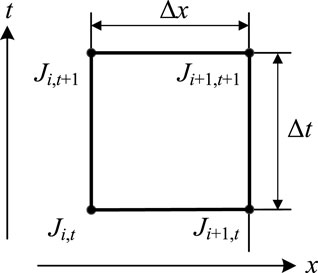
FIGURE 1. Finite difference cell of function $J(x,t)$

According to the differential linearization method, the simplified momentum equation and material balance equation of the blended gas, i.e. Eqs 17, 18 can be transferred into the following forms for each pipeline $ij$, while setting the spatial step and temporal step as the length of each pipe and 1 hour, respectively.

$\frac{1}{S_{ij}}[Q_{j,t+1}^{ij}+Q_{i,t+1}^{ij}-Q_{j,t}^{ij}-Q_{i,t}^{ij}]+\frac{\mathrm{\Delta }t}{L_{ij}}(P_{j,t+1}-P_{i,t+1}+P_{j,t}-P_{i,t})+\frac{\lambda {\overline{v}}_{ij}\Delta t}{4D_{ij}{S}_{ij}}[Q_{j,t+1}^{ij}+Q_{i,t+1}^{ij}+Q_{j,t}^{ij}+Q_{i,t}^{ij}]=0(20)$

$\frac{1}{c^2}(P_{j,t+1}+P_{i,t+1}-P_{j,t}-P_{i,t})+\frac{\mathrm{\Delta }t}{L_{ij}{S}_{ij}}[Q_{j,t+1}^{ij}-Q_{i,t+1}^{ij}+Q_{j,t}^{ij}-Q_{i,t}^{ij}]=0(21)$

where index $i$ and j indicate the front node and the end node of pipeline $ij$, respectively; $D_{ij}$, $S_{ij}$ and $L_{ij}$ represent the diameter, cross-sectional area, and length of the pipeline $ij$, respectively; ${\overline{v}}_{ij}$ represents the average flow velocity of blended gas in the pipeline $ij$; $P_{i,t}$ represents the pressure at the node $i$ of the pipeline and at time $t$; $Q_{i,t}^{ij}$ represents the mass flow rate of blended gas at the front node of pipeline $ij$ at time $t$ and $Q_{j,t}^{ij}$ represents the mass flow rate of blended gas at the end node of pipeline $ij$ at time $t$.

3 Schedule Optimization Model Without Uncertainty

In this section, the schedule optimization framework without considering the uncertainty for the IEGSH is established. The objective and operation constraints are introduced as follows.

3.1 Objective

The objective of the established schedule optimization model is to minimize the total operation cost of the IEGSH, and the objective function is as follows.

$\min F_E+F_G(22)$

where $F_E$ and $F_G$ indicate the operation cost of the power system and the operation cost of the natural gas system, respectively. The calculation formulas of $F_E$ and $F_G$ are shown as Eqs 23, 24.

$F_E={\displaystyle \sum _{t=1}^T{\displaystyle \sum _{i=1}^{N_g}(C^{coal}{F}_{i,t}^{coal}+C_i^{ud}{U}_{i,t}^{ud})}}(23)$

$F_G={\displaystyle \sum _{t=1}^T{\displaystyle \sum _{i=1}^{N_{\mathrm{gs}}}(C^M{Q}_{i,t}^{Ms}+C^H{Q}_{i,t}^{Hs})\mathrm{\Delta }}}t(24)$

where $T$ represents the amount of the time intervals; $N_g$ and $N_{gs}$ represent the quantity of the coal-fired generators in the power system and source nodes in the natural gas system, respectively;$C^{coal}$, $C^M$ and $C^H$ represent the price of coal, natural gas, and hydrogen, respectively; $F_{i,t}^{coal}$ represents the coal consumption of the coal-fired generator $i$ during the time interval $t$; $C_i^{ud}$ represents the cost of unit start-up and shut-down operation for generation $i$; $U_{i,t}^{ud}$ represents the start-up and shut-down operation of the coal-fired generator $i$ during the time interval $t$, which is a binary variable and equals to 1 when the on/off state of the coal-fired generator $i$ during the time interval $t$ is different from that during the time interval $t-1$; $Q_{i,t}^{Ms}$ and $Q_{i,t}^{Hs}$ represent the mass flow rate of methane and hydrogen at the gas source node $i$ during the time interval $t$, respectively.

3.2 Natural Gas System Constraints

The blended gas in each pipeline is supposed to meet the dynamic energy flow equations, i.e. Eqs 20, 21, in order to describe the pipeline transmission process with more accuracy. Besides, the following constraints should also be met to ensure the safety of pipeline operation.

3.2.1 Gas Load Constraints

The gas load at each sink node is known and it is given in the form of mass flow rate, i.e. $Q_{i,t}^L$. Considering the hydrogen blending, the following constraints are supposed to be met.

$Q_{j,t}^L{H}_M=\frac{K}{K+1}{Q}_{j,t}^{Lb}{H}_H+\frac{1}{K+1}{Q}_{j,t}^{Lb}{H}_M\forall j\in \sin \mathrm{k}\mathrm{n}\mathrm{o}\mathrm{d}\mathrm{e}\mathrm{s}(25)$

$Q_{j,t}^{ij}=Q_{j,t}^{Lb}\forall j\in \sin \mathrm{k}\mathrm{n}\mathrm{o}\mathrm{d}\mathrm{e}\mathrm{s}(26)$

where $H_H$ and $H_M$ represent the calorific value of the hydrogen and methane, respectively; $Q_{i,t}^{Lb}$ represents the mass flow rate of blended gas load at sink node $i$ and time interval $t$, which is determined according to the principle that total energy of the gas load is equivalent.

3.2.2 Source Node Pressure Constraints

The quality of the blended gas at each source node keeps consistent and hence the pressure and density of the gas at each source node are set to constant values.

$\{\begin{array}{l}{P}_{i,t}=P_i^s\\ {\rho }_{i,t}={\rho }_i^s\end{array}\forall i\in \mathrm{s}\mathrm{o}\mathrm{u}\mathrm{r}\mathrm{c}\mathrm{e}\mathrm{n}\mathrm{o}\mathrm{d}\mathrm{e}\mathrm{s}(27)$

where $P_i^s$ and ${\rho }_i^s$ represent the pressure and density of blended gas at the gas source node $i$.

3.2.3 Mass Flow Rate Balance Constraints

The amount of incoming mass flow rates or outgoing mass flow rates for each link node of the pipeline along every pipe should equal to 0, which keeps the mass flow rate balanced.

${\displaystyle \sum _{j=1}^{J_i}{Q}_{i,t}^{ij}}+{\displaystyle \sum _{k=1}^{K_i}{Q}_{i,t}^{ki}}=0(28)$

where $J_i$ represents the number of pipes, whose front node is the link node $i$; and $K_i$ represents the number of pipes, whose end node is the link node $i$.

3.2.4 Gas State Equation Constraints

For the gas at every node of the natural gas pipeline, the pressure and density must meet the gas state equation.

$P_{i,t}=c^2{\rho }_{i,t}(29)$

3.3 Power System Constraints

Besides the operation and safety constraints for the natural gas system, the power system must also meet the essential constraints to ensure the safe operation of the power system and the integrated energy system. The relevant constraints are listed in this section.

3.3.1 Power Balance Constraints

The power energy flow must remain balanced, which means the energy supplied by the generators equals to the energy consumed by the electric load.

${\displaystyle \sum _{i=1}^{N_g}{P}_{i,t}^g+{\displaystyle \sum _{i=1}^{N_{\mathit{GFU}}}{P}_{i,t}^{GFU}}}+{\displaystyle \sum _{i=1}^{N_w}{P}_{i,t}^w}={\displaystyle \sum _{i=1}^{N_{el}}{P}_{i,t}^l}+{\displaystyle \sum _{i=1}^{N_{P2G}}{P}_{i,t}^{P2G}}(30)$

where $N_{\mathit{g}}$, $N_{GFU}$, $N_w$, $N_{el}$, and $N_{\mathit{P}2\mathit{G}}$ represent the number of positions in which the coal-fired generator, gas-fired generator, wind farm, electric load, and P2G unit are placed in the power system, respectively;$P_{i,t}^g$, $P_{i,t}^{GFU}$, $P_{i,t}^w$, $P_{i,t}^l$, and $P_{i,t}^{P2G}$ represent the output electrical power of coal-fired generator $i$, the output electrical power of gas-fired generator $i$, the output electrical power of wind generator $i$, the electrical power consumption of electrical load $i$, and the input electrical power of P2G unit $i$ during time interval $t$, respectively.

3.3.2 Transmission Capacity Constraints

The direct current (DC) power flow is utilized in this work to determine the power flowing through power lines. Based on the DC power flow model, the transmission capacity constraints for power lines can be formulated as follows.

$f_{mn,t}={\mathbf{S}}_{mn}{\mathbf{P}}_t(31)$

$-f_{mn,t}^m\le f_{mn,t}\le f_{mn,t}^m(32)$

where $f_{mn,t}$ represents the power flowing through power line $mn$ during time interval $t$; $f_{mn,t}^m$ represents the limitation of power flowing through power line $mn$ during time interval $t$; ${\mathit{S}}_{\mathit{m}\mathit{n}}$ represents the row vector in power transfer distribution factors (PTDF) matrix corresponding to power line $mn$; and ${\mathit{P}}_{\mathit{t}}$ represents the column vector of input power at each node in the power system during the time interval $t$.

3.3.3 Operation Power Limitation Constraints

The output power of each generation should also be limited in its operating region.

$u_{i,t}{P}_{\mathit{min}i}^g\le P_{i,t}^g\le u_{i,t}{P}_{\mathit{max}i}^g\forall i\in \mathrm{coal}-\mathrm{fired\; generator\; nodes}(33)$

$P_{\min i}^{GFU}\le P_{i,t}^{GFU}\le P_{\max i}^{GFU}\forall i\in \mathrm{gas}-\mathrm{fired\; generator\; nodes}(34)$

$P_{\min i}^{P2G}\le P_{i,t}^{P2G}\le P_{\max i}^{P2G}\forall i\in \mathrm{P2G}\mathrm{nodes}(35)$

where $u_{i,t}$ represents the on/off state for coal-fired generator $i$ during time interval $t$ and equals to 1 when the generator is on; $P_{\min i}^g$ and $P_{\max i}^g$ represent the minimal and maximal output power limitation for coal-fired generator $i$, respectively; $P_{\min i}^{GFU}$ and $P_{\max i}^{GFU}$ represent the minimal and maximal output power limitation for gas-fired generator $i$, respectively; $P_{\min i}^{P2G}$ and $P_{\max i}^{P2G}$ represent the minimal and maximal input power limitation for P2G unit $i$, respectively.

3.3.4 Start-Up and Shut-Down Time Duration Constraints

The time duration of being start-up and shut-down for coal-fired generators is supposed to be limited in the required range.

$u_{i,t-1}\le u_{i,t}\forall i\in \mathrm{coal}-\mathrm{fired\; generator\; nodes},t\le T_i^{on}(36)$

$u_{i,t}\le u_{i,t-1}\forall i\in \mathrm{coal}-\mathrm{fired\; generator\; nodes},t\le T_i^{off}(37)$

$(u_{i,t-1}-u_{i,t})T_i^{on}\le {\displaystyle \sum _{\tau =t-T_i^{on}}^{t-1}{u}_{i,\tau }}\forall i\in \mathrm{coal}-\mathrm{fired\; generator\; nodes},t\ge T_i^{on}+1(38)$

$(u_{i,t}-u_{i,t-1})T_i^{off}\le {\displaystyle \sum _{\tau =t-T_i^{off}}^{t-1}(1-u_{i,\tau })}\forall i\in coal-firedgeneratornodes,t\ge T_i^{off}+1(39)$

where $T_i^{on}$ and $T_i^{off}$ represent the minimal time duration of being start-up and shut-down for coal-fired generator $i$, respectively.

3.3.5 Ramp Rate Constraints

The ramp rate constraints for coal-fired generators can be depicted as follows.

$P_{i,t}^g-P_{i,t-1}^g\le R_i^U+(1-u_{i,t})M\forall i\in \mathrm{coal}-\mathrm{fired\; generator\; nodes}(40)$

$P_{i,t-1}^g-P_{i,t}^g\le R_i^D+(1-u_{i,t-1})M\forall i\in \mathrm{coal}-\mathrm{fired\; generator\; nodes}(41)$

where $R_i^U$ and $R_i^D$ represent the maximal up and down ramp rates for coal-fired generator $i$, and $M$ represents a large number which is much larger than other parameters and variables in the model.

3.3.6 State of Generator Constraints

The state of the coal-fired generators should meet the following constraints. When the on/off state of the coal-fired generator $i$ during the time interval $t$ is different from that during the time interval $t-1$, $U_{i,t}^{ud}=1$, otherwise, $U_{i,t}^{ud}=0$. And the on/off state change during the first time interval is neglected, i.e. $U_{i,1}^{ud}=0$.

$U_{i,1}^{ud}=0\forall i\in \mathrm{coal}-\mathrm{fired\; generator\; nodes}(42)$

$U_{i,t}^{ud}\ge u_{i,t-1}-u_{i,t}\forall i\in \mathrm{coal}-\mathrm{fired\; generator\; nodes}(43)$

$U_{i,t}^{ud}\ge u_{i,t}-u_{i,t-1}\forall i\in \mathrm{coal}-\mathrm{fired\; generator\; nodes}(44)$

3.4 Energy Conversion Constraints

In the IEGS, the GFU and P2G units play a very important role in coupling the energy flow of different systems. With the hydrogen blending to the traditional natural gas system, the P2G unit can be classified into two categories, i.e. P2M unit and P2H unit. In order to guarantee co-operation safety, the constraints for the energy coupling units must also be met and they are discussed as follows.

3.4.1 Gas-Fired Unit Operation Constraints

The output power of GFU is associated with consumed gas by its efficiency coefficient. In this work, hydrogen is injected into the natural gas system. Therefore, the gas consumed by the GFU is blended gas of hydrogen and methane. Based on the assumption that the volume ratio of hydrogen blending in the natural gas pipeline, i.e. $R_V$, keeps constant and meanwhile the volume ratio $R_V$ is not very large, the GFUs in the system are assumed to be able to utilize the mixed gas directly. The operation of the GFUs is supposed to meet the following constraints.

$P_{i,t}^{GFU}={\eta }_i^{GFU}{Q}_{i,t}^{GFU}\forall i\in \mathrm{gas}-\mathrm{fired\; generator\; nodes}(45)$

$Q_{i,t}^{GFU}=Q_{i,t}^{ki}\forall i\in \mathrm{gas}-\mathrm{fired\; generator\; nodes}(46)$

where $Q_{i,t}^{GFU}$ represents the mass flow rate of gas flowing into gas-fired generator $i$ during time interval $t$; and ${\eta }_i^{GFU}$ represents the energy conversion efficiency coefficient of the gas-fired generator $i$.

Eq. 45 describes the relationship between the output power of gas-fired generator $i$ and the mass flow rate of gas consumed by it.

3.4.2 Power-To-Gas Unit Operation Constraints

The P2M unit and P2H unit are both required to meet the corresponding operation constraints.

$Q_{i,t}^{P2M}={\eta }_i^{P2M}{P}_{i,t}^{P2M}\forall i\in \mathrm{P2G}\mathrm{nodes}(47)$

$Q_{i,t}^{P2H}={\eta }_i^{P2H}{P}_{i,t}^{P2H}\forall i\in \mathrm{P2G}\mathrm{nodes}(48)$

$Q_{i,t}^{P2M}=-\frac{1}{K+1}{Q}_{i,t}^{ki}\forall i\in \mathrm{P2G}\mathrm{nodes}(49)$

$Q_{i,t}^{P2H}=-\frac{K}{K+1}{Q}_{i,t}^{ki}\forall i\in \mathrm{P2G}\mathrm{nodes}(50)$

$P_{i,t}^{P2G}=P_{i,t}^{P2M}+P_{i,t}^{P2H}\forall i\in \mathrm{P2G}\mathrm{nodes}(51)$

where $Q_{i,t}^{P2M}$ represents the mass flow rate of methane produced by the P2M unit $i$ during time interval $t$; $P_{i,t}^{P2M}$ represents the electric power consumed by the P2M unit $i$ during time interval $t$; ${\eta }_i^{P2M}$ represents the energy conversion efficiency coefficient of the P2M unit $i$; $Q_{i,t}^{P2H}$ represents the mass flow rate of hydrogen produced by the P2H unit $i$ during time interval $t$; $P_{i,t}^{P2H}$ represents the electric power consumed by the P2H unit $i$ during time interval $t$; ${\eta }_i^{P2H}$ represents the energy conversion efficiency coefficient of the P2H unit $i$. And the minus sign of the mass flow rate in Eqs 49, 50 results from that the mass flow rate of gas produced by the P2G unit is regarded as gas load for the natural gas system in this work.

3.5 Summary of the Deterministic Schedule Optimization Problem

According to the above analysis, the model of the deterministic schedule optimization problem can be summarized as follows.

Objective: (22)

Subject to:

Natural gas system constraints: (20), (21), (25)–(29)

Power system constraints: (30)–(41)

Energy conversion constraints: (45)–(51)

4 Robust Scheduling Methodology

The deterministic schedule optimization model for the IEGSH is formulated in Section 3 and the form of the model is described as Eq. 52.

$\begin{array}{l}\min {\mathbf{c}}^T[\mathbf{x};\mathbf{u}]\\ \mathrm{s.t}.\mathbf{A}\mathbf{x}+\mathbf{B}\mathbf{u}+\mathbf{C}\mathbf{w}\le \mathbf{b}\end{array}(52)$

where $\mathbf{c}$ represents the column vector consisting of coefficient of the objective function; $\mathbf{u}$ and $\mathbf{x}$ represent the column vector consisting of decision variables of on/off state for coal-fired generators and the column vector consisting of all other decision variables; $\mathbf{w}$ represents the column vector consisting of output power for wind generators;$\mathbf{A}$, $\mathbf{B}$ and $\mathbf{C}$ represent coefficient matrix of decision variables and output wind power for all considered constraints; $\mathbf{b}$ represents the constant column vector.

In model (52), the uncertainty of parameters is not considered and the uncertainty of the wind power is taken into consideration in this section. To optimize the day-ahead schedule with economic efficiency, high reliability, and safety, a two-stage robust schedule optimization method is established. The unit commitment (UC) master problem in the deterministic scenario is optimized in the first stage, which is with the similar form of Eq. 52. The UC plan determined in the first stage acts as the known parameter for the feasibility sub-problem in the second stage. Then the robust feasibility of the UC plan is verified and the feasible cut is added into the UC problem in the first stage. And the robust problem for day-ahead scheduling is solved iteratively by the C&CG algorithm.

4.1 Feasibility Sub-problem

Feasibility sub-problem aims to validate the robust feasibility when the wind power is of uncertainty. The formulation of the feasibility sub-problem based on Eq. 52 is shown as Eq. 53.

$\begin{array}{l}\underset{w}{\max }\underset{x,s}{\min }{d}^T[x;w;s]\\ \mathrm{s.t}.Ax+B{u}^{\ast }+Cw+Ds\le b\\ \underset{¯}{w}\le w\le \stackrel{—}{w}\\ s\ge 0\end{array}(53)$

where s is a column vector of slack variables introduced to ensure the problem feasible; ${\mathbf{u}}^{\ast }$ represents the column vector consisting of decision variables of on/off state for coal-fired generators determined by the master problem; $\mathbf{d}$ is a column vector, whose value of elements corresponding to $\mathbf{x}$ and $\mathbf{w}$ equals to 0 and value of elements corresponding to $s$ equals to 1; $\mathbf{D}$ represents the coefficient matrix of slack variables for considered constraints; $\underset{¯}{w}$ and $\overline{w}$ represent column vector of upper and lower bound for the fluctuation range of wind power.

The main constraints of the feasibility sub-problem are the same as the master problem, except that $\mathbf{u}$ is already determined and the $\mathbf{w}$ is of uncertainty. However, the constraints relevant with $\mathbf{u}$ should be modified and added the slack variables.

$P_{i,t}^{\mathit{gw}}+s_{i,t}^1\ge u_{i,t}^{\ast }{P}_{\mathit{min}i}^g\forall i\in \mathrm{coal}-\mathrm{fired\; generator\; nodes}(54)$

$P_{i,t}^{\mathit{gw}}-s_{i,t}^2\le u_{i,t}^{\ast }{P}_{\mathit{max}i}^g\forall i\in \mathrm{coal}-\mathrm{fired\; generator\; nodes}(55)$

$P_{i,t}^{\mathit{gw}}-P_{i,t-1}^{\mathit{gw}}-s_{i,t}^3\le R_i^U+(1-u_{i,t}^{\ast })M\forall i\in \mathrm{coal}-\mathrm{fired\; generator\; nodes}(56)$

$P_{i,t-1}^{\mathit{gw}}-P_{i,t}^{\mathit{gw}}-s_{i,t}^4\le R_i^D+(1-u_{i,t-1}^{\ast })M\forall i\in \mathrm{coal}-\mathrm{fired\; generator\; nodes}(57)$

where $P_{i,t}^{\mathit{gw}}$ represents the output electrical power of coal-fired generator $i$ during time interval $t$ in the scenario considering the uncertainty of wind power; $s_{i,t}^{(\cdot )}$ represents the slack variable.

The objective function of the sub-problem must equal to a positive value owing to that all elements of s are not less than 0. the UC plan determined by the master problem can ensure the operation of the IEGSH safe and reliable, which means that the ahead-day scheduling is of enough robustness to deal with all uncertain wind power scenarios, when the objective function equals to 0. Otherwise, there is at least an uncertain wind power scenario in which some constraints cannot be met, because there is at least a slack variable that doesn’t equal to 0.

The sub-problem is a two-level optimization problem, whose inner level is a minimization problem and outer level is a maximization problem, and the objective function of the inner and outer problem is the same. In order to solve the two-level optimization problem, the inner minimization problem can be transferred into its dual problem, which is a maximization problem.

$\begin{array}{l}\underset{w,y}{\max }{y}^{\mathit{T}}(B{u}^{\ast }+Cw-b)\\ \mathrm{s.t}.{[A,D]}^{\mathit{T}}y+b=0\\ y\ge 0\\ \underset{¯}{w}\le w\le \stackrel{—}{w}\end{array}(58)$

where y represents the column vector consisting of dual variables of the primal problem.

The existence of the multiply term of $\mathbf{y}$ and $\mathbf{w}$ makes the objective function nonlinear, which also makes the problem hard to be solved. In this work, a linearization method is used to deal with this problem.

The box uncertainty set is used to describe the fluctuation range of wind power. The schedule plan is robust enough to deal with the uncertainty when the relevant constraints can be met in the extreme scenario. The extreme scenario for wind power can be described as follows.

$\{\begin{array}{l}{\mathrm{w}}_i={\underset{¯}{\mathrm{w}}}_i+{\mathrm{I}}_i\mathrm{\Delta }{\mathrm{w}}_i\\ \mathrm{\Delta }{\mathrm{w}}_i={\overline{\mathrm{w}}}_i-{\underset{¯}{\mathrm{w}}}_i\\ {\overline{\mathrm{w}}}_i=(1+{\mathrm{\alpha }}^{+}){\mathrm{w}}^{\mathit{p}}\\ {\underset{¯}{\mathrm{w}}}_i=(1-{\mathrm{\alpha }}^{-}){\mathrm{w}}^{\mathit{p}}\end{array}(59)$

where $w_i$ represents the element $i$ in $\mathbf{w}$; ${\underset{¯}{w}}_i$ and ${\overline{w}}_i$ represent the upper and lower bound for fluctuation range of $w_i$; $w^p$ represents the forecast value of $w_i$; ${\alpha }^{+}$ and ${\alpha }^{-}$ represent the positive and negative fluctuation ratio of $w_i$ relative to $w^p$; $I_i$ represents binary variable to determine the value of $w_i$.

Therefore, the nonlinear term of in Eq. 58 can be transferred into the following form.

$y^{\mathit{T}}Cw=y^{\mathit{T}}C(\underset{¯}{w}+I\mathrm{\Delta }w)=y^{\mathit{T}}C\underset{¯}{w}+y^{\mathit{T}}CI\mathrm{\Delta }w(60)$

where $\mathbf{I}$ represents the set consisting of all $I_i$.

Introduce the auxiliary variable vector ${\mathbf{w}}_a$ to indicate the term of $\mathbf{C}\mathbf{I}\Delta \mathbf{w}$ and constraint ${\mathbf{w}}_a$ as Eq. 61 to linearize the term of ${\mathbf{y}}^T\mathbf{C}\mathbf{I}\Delta \mathbf{w}$.

$\{\begin{array}{c}-M\mathbf{I}\le {\mathbf{w}}_a\le M\mathbf{I}\\ \mathbf{C}\mathrm{\Delta }\mathbf{w}-M(1-\mathbf{I})\le {\mathbf{w}}_a\le \mathbf{C}\mathrm{\Delta }\mathbf{w}+M(1-\mathbf{I})\end{array}(61)$

Based on the above analysis, the sub-problem can be transferred into the following form, which is a linear programming problem and can be solved more easily.

$\begin{array}{l}\underset{w,y}{\max }{y}^T(B{u}^{\ast }-b+C\underset{¯}{w}+w_a)\\ \mathrm{s.t}.{[A,D]}^{T}y+b=0\\ y\ge 0\\ -\mathit{M}\mathit{I}\le w_a\le \mathit{M}\mathit{I}\\ C\mathrm{\Delta }w-\mathit{M}(1-I)\le w_a\le C\mathrm{\Delta }w+\mathit{M}(1-I)\end{array}(62)$

4.2 Column-and-Constraint Generation Iterative Algorithm

The robust schedule optimization model established in this paper consists of the master problem and feasibility sub-problem and an iterative solving method based on the C&CG algorithm is proposed to solve the problem. The scheme of the method is illustrated in Figure 2 and the specific steps of implementation are as follows:

FIGURE 2

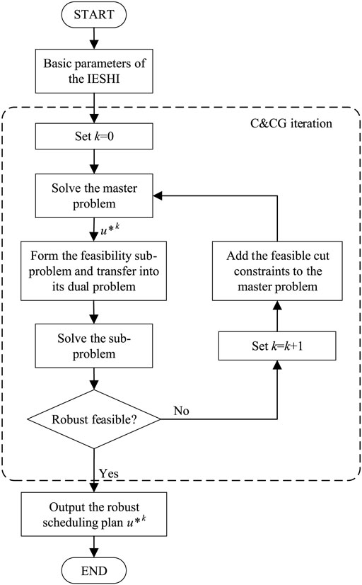
FIGURE 2. Scheme of the C&CG iteration algorithm.

Step 1. Construct the structure and input the basic parameters of the IEGSH and equipment. Initialize the model and set k = 0.

Step 2. Solve the master problem at the scenario with the forecast wind power and determine the UC plan u^*k.

Step 3. Solve the feasibility sub-problem and validate the feasibility of the UC plan u^*k by comparing the objective value, i.e. ${\displaystyle \sum s}$, with the convergence error $\epsilon$.

Step 4. The result ${\displaystyle \sum s}\le \epsilon$ means that the UC plan u^*k can meet the robust requirement for all wind power scenarios and then the UC plan u^*k can be outputted as the robust day-ahead schedule.

Step 5. The result ${\displaystyle \sum s}>\epsilon$ means that there is at least one scenario at which the UC plan u^*k cannot meet the required constraints. Therefore, set k = k+1 and generate and add new feasible cut constraints into the master problem. Then go back to Step 2. The forms of the feasible cut constraints are shown as follows and w^k represents the wind power at the extreme scenario.

$Ax+Bu+C{w}^k\le b(63)$

5 Results and Discussion

In this work, the IEGSH built as the test system consists of the IEEE 39-bus power system, shown in Figure 3, and the 27-node natural gas system, shown in Figure 4. There are 29 branches and 26 pipes in the power system and natural gas system, respectively. There are totally 10 generators in the power system and the generators at Bus 32 and 33 are GFUs, connected to Node 13 and 22 in the natural gas system, both with capacities of 400 MW and the efficiencies are 16.5 MW/(kg/s) and 19.8 MW/(kg/s). The generators at Bus 35 and 38 are wind farms. The 2 P2G units, including P2M and P2H unit, are located in Bus 17 and 22, which are connected to Node 27 and 8 in the natural gas system, both with capacities of 400 MW and comprehensive efficiencies are 0.0055 (kg/s)/MW and 0.0064 (kg/s)/MW. The parameters of coal-fired generators are shown in Table 1. The day-ahead forecast curve of wind power and electric load power curve and the natural gas load curve used in this work are shown in Figure 5 and Figure 6, respectively. The blending volume ratio of hydrogen into the natural gas pipeline is set as 5%. And the price of coal, natural gas, and hydrogen are set as 500 CNY/t, 2 CNY/kg, and 20 CNY/kg. And the convergence error ε is set as 0.0001.

FIGURE 3

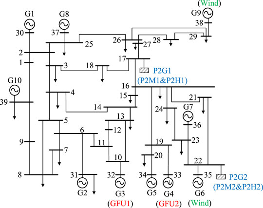
FIGURE 3. The topology of the electric system in IEGSH.

FIGURE 4

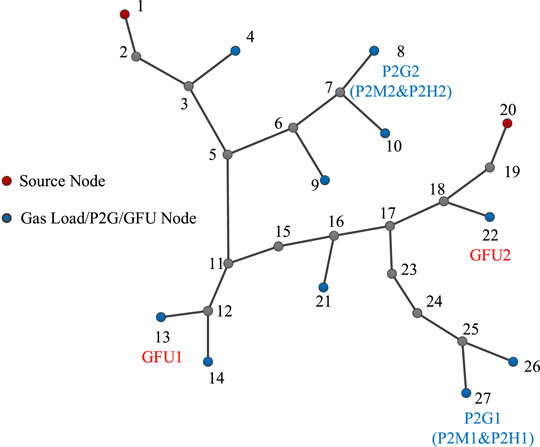
FIGURE 4. The topology of the natural gas system in IEGSH.

TABLE 1

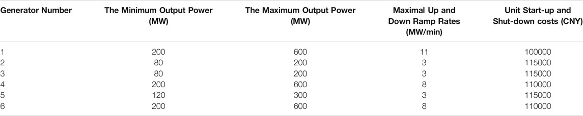
TABLE 1. The parameters of the coal-fired generators in the IEGSH.

FIGURE 5

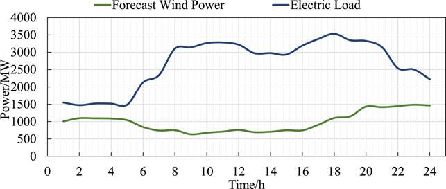
FIGURE 5. The day-ahead forecast curve of wind power and electric load power curve.

FIGURE 6

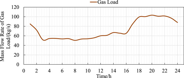
FIGURE 6. The natural gas load curve.

In this study, two cases, i.e. deterministic and stochastic cases, are set to validate the effectiveness and feasibility of the proposed method. In the deterministic case, the uncertainty of the parameter is not considered, and the day-ahead schedule is optimized by the model established in Section 3. In the stochastic case, the uncertainty of the wind power is taken into consideration and the maximum fluctuation deviation is set as ±50%, and the day-ahead schedule determined by the robust model proposed in Section 4 can deal with the uncertainty of wind power to guarantee the operation safety, reliability of electricity supply and accommodation of wind power.

5.1 Deterministic Case

The schedule of UC plan for coal-fired generators determined in the deterministic case is shown in Figure 7 and the optimal operation strategy is shown in Figure 8. The operation cost for the corresponding operation strategy is shown in the second column of Table 2. In Figure 7, the on/off states of each coal-fired generator for each time interval are indicated by the colored dot and the colored dot during one time interval means that the corresponding generator is turned on during that time interval. As Figure 7 shows, there are 3 coal-fired generators turned on during the whole day while the other 3 coal-fired generators are turned off during the day, therefore, the start-up and shut-down cost is 0. In Figure 8, the output and consumption power of each equipment for each time interval are indicated by the height of the colored bar, and the consumption power of P2G units is regarded as minus output power. The electric energy supplied by coal-fired generators, GFUs, wind farms, and consumed by P2G units during the whole day are 29793.09 MWh, 12170.32 MWh, 23738.80 MWh, and 1611.65 MWh, respectively. The costs for purchasing coal and gas are 4539314 CNY and 10242638 CNY, while the total operation cost for IEGSH is 14781952 CNY.

FIGURE 7

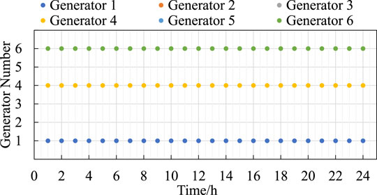
FIGURE 7. The day-ahead schedule of coal-fired generators in the deterministic case.

FIGURE 8

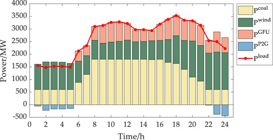
FIGURE 8. The day-ahead operation strategy for electric system in the deterministic case.

TABLE 2

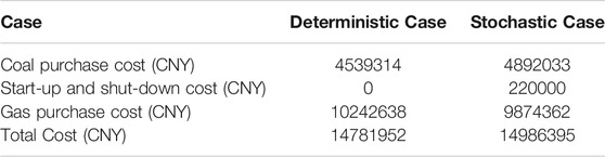
TABLE 2. The operation cost of different cases.

The adoption of the dynamic energy flow equations for the natural gas system can describe the dynamic operation process of gas in the gas pipeline. And the analysis of the dynamic transmission process is carried out as follows. Taking pipe 3–5, of which Node 3 is the front and Node 5 is the end, as an example, the mass flow rate of the gas flowing through this pipe and the pressures at its two ends are depicted in Figure 9. As Figure 9A shows, the mass flow rates of the gas outgoing the Node 3 and incoming the Node 5 do not necessarily equal to each other at each time interval, owing to the dynamic characteristic of gas is considered. However, the mass flow rates of gas at the front and end of each pipe are the same in many previous studies, in which the steady-state model of natural gas system is applied.

FIGURE 9

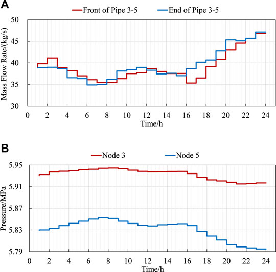
FIGURE 9. The dynamic energy flow through pipe 3–5 of the natural gas system. (A) The mass flow rate at the front and end of pipe 3–5. (B) The pressure of gas at Node 3 and Node 5.

The fact that the pressure of the pipe increases when the outgoing mass flow rate of gas at its front node along the pipe is larger than the incoming mass flow rate of gas at its end node along the pipe and vice versa is obvious. Figure 9B depicts the changes of the pressures of the gas at Node 3 and Node 5. By comparing changes of the mass flow rates and pressures, it can be noticed that the pressure of the pipe increases between 1:00 and 8:00 and the outgoing mass flow rate of gas at Node 3 along the pipe 3-5 is larger than the incoming mass flow rate of gas at Node 5 along the pipe 3-5 in this time period, which is consistent with the theory. The similar conclusions can be drawn during other time periods in the day.

5.2 Stochastic Case

The schedule of UC plan for coal-fired generators determined in the stochastic case is shown in Figure 10 and the optimal operation strategy is shown in Figure 11. The operation cost for the corresponding operation strategy is shown in the third column of Table 2. Similar to Figure 7, in Figure 10, the colored dot during one time interval means that the corresponding coal-fired generator is turned on during that time interval. As Figure 10 shows, there are 4 coal-fired generators turned on during the whole day while one coal-fired generator is turned off during the day and the other one coal-fired generator starts up at 7:00 and shuts down at 19:00. And the start-up and shut-down cost is 220000 CNY, different from that in the deterministic case.

FIGURE 10

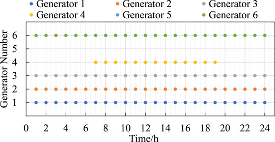
FIGURE 10. The day-ahead schedule of coal-fired generators in the stochastic case.

FIGURE 11

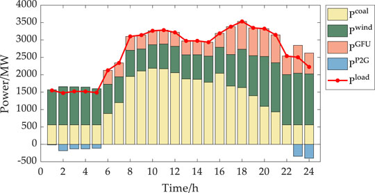
FIGURE 11. The day-ahead operation strategy for electric system in the stochastic case.

In Figure 11, the output and consumption power of each equipment for each time interval are also indicated by the height of the colored bar. The electric energy supplied by coal-fired generators during the whole day is 31332.49 MWh, which is more than that in the deterministic case. The electric energy supplied by GFUs during the whole day is 10334.14 MWh, which is less than that in the deterministic case. The electric energy consumed by P2G units during the whole day is 1314.85 MWh. The difference between the two cases results from the reason that more coal-fired generators are supposed to be turned on to guarantee the reliability of electricity supply and accommodation of wind power when the IEGSH suffers extreme uncertainty.

As Table 2 shows, the costs for purchasing coal and gas are 4892033 CNY and 9874362 CNY. The total operating cost for IEGSH is 14986395 CNY, which is 204443 CNY more than that in the deterministic case to promote the robustness of the system.

5.3 Robustness Validation of the Proposed Robust Schedule Optimization Model

As for the same forecast curve of wind power, the operation cost of schedule determined by the proposed robust schedule optimization model is more than that determined by the deterministic model, which means the operation strategy is less economically efficient but more robust. To validate the superiority of the proposed robust schedule optimization model in promoting the robustness of the IEGSH, the following works are carried out.

Figure 12 illustrates the ten wind power curves generated to act as the intra-day actual operation scenarios, which are all among the maximum $\pm 50\%$ uncertainty fluctuation range. It can be seen that all wind power curves are between the upper and lower fluctuation bound curves. The validation model is similar to the deterministic model proposed in Section 3 but the objective is changed into minimizing the sum of wind curtailment and electric load curtailment. Besides, the schedule of UC plan for coal-fired generators determined in the deterministic and stochastic case are chosen as the determined intra-day schedule, respectively.

FIGURE 12

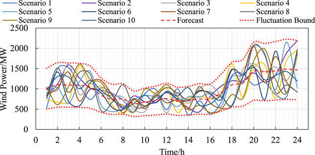
FIGURE 12. The wind power curves in the ten scenarios generated and the forecast scenario.

As for the UC plan determined in the deterministic case, the solving results for the ten intra-day wind power scenarios are shown in Table 3. It can be seen that there is load curtailment in all generated scenarios and wind curtailment in scenarios 2 and 5. The maximum load curtailment is up to 796.53 MWh and the reliability of electric supply is weak, which means the schedule is of poor robustness.

TABLE 3

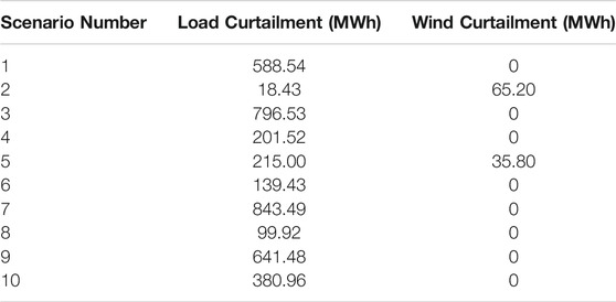
TABLE 3. The load curtailment and wind curtailment for the UC plan determined by the deterministic model in the generated scenarios.

Different from the situation in the deterministic case, there is only 12.06 MWh load curtailment in the scenario 6 and the load curtailment and wind curtailment in other scenarios all equal to 0 when the schedule of UC plan determined by the robust model is chosen as the intra-day schedule, which indicates that the robustness of the day-head schedule is of great robustness.

5.4 Carbon Emission Reduction Resulting From Hydrogen Blending

The P2H unit can produce hydrogen by using renewables, which can promote the accommodation of the renewables and blend the hydrogen into the natural gas pipeline to realize the storage and transportation of hydrogen. It can not only reduce the investment cost of the specific pipeline but also reduce the carbon emission during the utilization of the natural gas because the hydrogen blended in the methane is clean energy.

To quantify the benefit of blending hydrogen, set the discounted standard coal coefficient of methane and carbon emission coefficient of standard coal as 1.674 t standard coal/t and 2.66 t CO₂/t standard coal, respectively. As for the operation strategy optimized by the deterministic model and robust model, the corresponding CO₂ emission can be calculated and is shown in Table 4. The CO₂ emissions of the deterministic and stochastic operation strategy are 46883.02 t and 47942.08 t when considering the involvement of hydrogen, respectively, which are 17.96 t and 17.31 t less than that of the situation without hydrogen blending.

TABLE 4

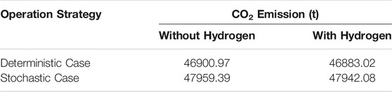
TABLE 4. The CO₂ emission at each operation strategy.

In the future, the hydrogen blend ratio will further increase and the hydrogen blending technology will be put into scale application as the corresponding technologies develop and mature. It can be foreseen that the hydrogen blending technology will be able to play a more and more important role in reducing carbon emission.

6 Conclusion

This paper focuses on the robust day-ahead schedule of the IEGS considering blending hydrogen. The energy flow model of natural gas system considering the dynamic characteristic of gas pipeline and blending of hydrogen is proposed. Further, a robust schedule optimization model is proposed and the solving method based on the C&CG algorithm is adopted to solve the problem. Then case studies on a test system combining a 39-bus electric system and a 27-node natural gas system verify the effectiveness and superiority of the proposed method. From the results of case studies, our findings and conclusions can be drawn: 1) The changes of the gas pressure and mass flow rate determined by the proposed dynamic energy flow model accord with the theory. The adoption of the dynamic energy flow equation for the gas in the pipeline can help ensure the operation safety of gas system because the description of gas transmission is more accurate. 2) The day-ahead schedule determined by the proposed robust optimization model is of less economic efficiency but much more robustness compared with the deterministic model. The reliability of electric supply and the accommodation of renewables can be ensured better by using the proposed methodology. 3) The blending hydrogen in the natural gas pipeline can reduce carbon emission during the operation of the IEGS owing to the non-pollution characteristic of hydrogen. The methodology proposed in this paper can help ensure the operation safety of the systems in scenarios with high uncertainty and give some reference for the development of blending hydrogen technology.

Data Availability Statement

The original contributions presented in the study are included in the article/Supplementary Material, further inquiries can be directed to the corresponding authors.

Author Contributions

All authors listed have made a substantial, direct, and intellectual contribution to this work and approved it for publication.

Funding

This work was supported by the State Grid Hubei Electric Power Company Limited under the Science and Technology Project Grant No. 521538210003. And the project is entitled “Research on Coordinated Planning Technology of Integrated Electric-Gas System for Renewable Energy Accommodation”.

Conflict of Interest

Authors DY, SW, HZ, DY, and JY are employed by State Grid Hubei Electric Power Company Limited Economic Research Institute.

The remaining authors declare that the research was conducted in the absence of any commercial or financial relationships that could be construed as a potential conflict of interest.

Publisher’s Note

All claims expressed in this article are solely those of the authors and do not necessarily represent those of their affiliated organizations, or those of the publisher, the editors and the reviewers. Any product that may be evaluated in this article, or claim that may be made by its manufacturer, is not guaranteed or endorsed by the publisher.

References

Bai, L., Li, F., Jiang, T., and Jia, H. (2016). Robust Scheduling for Wind Integrated Energy Systems Considering Gas Pipeline and Power Transmission N-1 Contingencies. IEEE Trans. Power Syst. 32 (2), 1. doi:10.1109/TPWRS.2016.2582684

CrossRef Full Text | Google Scholar

Ban, M., Yu, J., Shahidehpour, M., and Yao, Y. (2017). Integration of Power-To-Hydrogen in Day-Ahead Security-Constrained Unit Commitment with High Wind Penetration. J. Mod. Power Syst. Clean. Energ. 5 (3), 337–349. doi:10.1007/s40565-017-0277-0

CrossRef Full Text | Google Scholar

Brouwer, A. S., van den Broek, M., Seebregts, A., and Faaij, A. (2014). Impacts of Large-Scale Intermittent Renewable Energy Sources on Electricity Systems, and How These Can Be Modeled. Renew. Sustain. Energ. Rev. 33, 443–466. doi:10.1016/j.rser.2014.01.076

CrossRef Full Text | Google Scholar

Cong Liu, C., Shahidehpour, M., Yong Fu, Y., and Zuyi Li, Z. (2009). Security-constrained Unit Commitment with Natural Gas Transmission Constraints. IEEE Trans. Power Syst. 24 (3), 1523–1536. doi:10.1109/TPWRS.2009.2023262

CrossRef Full Text | Google Scholar

Ding, T., Hu, Y., and Bie, Z. (2018). Multi-stage Stochastic Programming with Nonanticipativity Constraints for Expansion of Combined Power and Natural Gas Systems. IEEE Trans. Power Syst. 33 (1), 317–328. doi:10.1109/TPWRS.2017.2701881

CrossRef Full Text | Google Scholar

Erdiwansyah, M., Mahidin, H., HusinZaki, H., Nasaruddin, Zaki, M., and Muhibbuddin, (2021). A Critical Review of the Integration of Renewable Energy Sources with Various Technologies. Prot. Control. Mod. Power Syst. 6 (1), 1–18. doi:10.1186/s41601-021-00181-3

CrossRef Full Text | Google Scholar

Fang, J., Zeng, Q., Ai, X., Chen, Z., and Wen, J. (2018). Dynamic Optimal Energy Flow in the Integrated Natural Gas and Electrical Power Systems. IEEE Trans. Sustain. Energ. 9 (1), 188–198. doi:10.1109/TSTE.2017.2717600

CrossRef Full Text | Google Scholar

Hang, S., Xiaomeng, A., Jinyu, W., Jiakun, F., Zhe, C., and Haibo, H. (2017). “Hybrid Approximate Dynamic Programming Approach for Dynamic Optimal Energy in the Integrated Gas and Power Systems,” in Paper presented at the 2017 IEEE conference on energy internet and energy system integration, Beijing,China, 26-28 Nov. 2017 (IEEE).

Google Scholar

He, C., Wu, L., Liu, T., and Shahidehpour, M. (2017). Robust Co-optimization Scheduling of Electricity and Natural Gas Systems via Admm. IEEE Trans. Sustain. Energ. 8 (2), 658–670. doi:10.1109/TSTE.2016.2615104

CrossRef Full Text | Google Scholar

Hu, Q., Lin, J., Zeng, Q., Fu, C., and Li, J. (2020). Optimal Control of a Hydrogen Microgrid Based on an experiment Validated P2hh Model. IET Renew. Power Generation 14 (3), 364–371. doi:10.1049/iet-rpg.2019.0544

CrossRef Full Text | Google Scholar

Jiang, Y., Xu, J., Sun, Y., Wei, C., Wang, J., Liao, S., et al. (2018). Coordinated Operation of Gas-Electricity Integrated Distribution System with Multi-Cchp and Distributed Renewable Energy Sources. Appl. Energ. 211, 237–248. doi:10.1016/j.apenergy.2017.10.128

CrossRef Full Text | Google Scholar

Kavadias, K. A., Kosmas, V., and Tzelepis, S. (2022). Sizing, Optimization, and Financial Analysis of a green Hydrogen Refueling Station in Remote Regions. Energies 15 (2), 547. doi:10.3390/en15020547

CrossRef Full Text | Google Scholar

Kim, M.-H., Kim, D.-W., and Lee, D.-W. (2021). Feasibility of Low Carbon Renewable Energy City Integrated with Hybrid Renewable Energy Systems. Energies 14 (21), 7342. doi:10.3390/en14217342

CrossRef Full Text | Google Scholar

Li, H., Ye, Y., and Lin, L. (2021). Low-carbon Economic Bi-level Optimal Dispatching of an Integrated Power and Natural Gas Energy System Considering Carbon Trading. Appl. Sci. 11 (15), 6968. doi:10.3390/app11156968

CrossRef Full Text | Google Scholar

Li, J., Lin, J., Song, Y., Xing, X., and Fu, C. (2019). Operation Optimization of Power to Hydrogen and Heat (P2hh) in Adn Coordinated with the District Heating Network. IEEE Trans. Sustain. Energ. 10 (4), 1672–1683. doi:10.1109/TSTE.2018.2868827

CrossRef Full Text | Google Scholar

Li, T., Eremia, M., and Shahidehpour, M. (2008). Interdependency of Natural Gas Network and Power System Security. IEEE Trans. Power Syst. 23 (4), 1817–1824. doi:10.1109/TPWRS.2008.2004739

CrossRef Full Text | Google Scholar

Li, Y., Zou, Y., Tan, Y., Cao, Y., Liu, X., Shahidehpour, M., et al. (2018). Optimal Stochastic Operation of Integrated Low-Carbon Electric Power, Natural Gas, and Heat Delivery System. IEEE Trans. Sustain. Energ. 9 (1), 273–283. doi:10.1109/TSTE.2017.2728098

CrossRef Full Text | Google Scholar

Liu, C., Shahidehpour, M., and Wang, J. (2011). Coordinated Scheduling of Electricity and Natural Gas Infrastructures with a Transient Model for Natural Gas Flow. Chaos 21 (2), 025102. doi:10.1063/1.3600761

PubMed Abstract | CrossRef Full Text | Google Scholar

Liu, J., Sun, W., and Harrison, G. (2019). Optimal Low-Carbon Economic Environmental Dispatch of Hybrid Electricity-Natural Gas Energy Systems Considering P2g. Energies 12 (7), 1355. doi:10.3390/en12071355

CrossRef Full Text | Google Scholar

Martinez-Mares, A., and Fuerte-Esquivel, C. R. (2012). A Unified Gas and Power Flow Analysis in Natural Gas and Electricity Coupled Networks. IEEE Trans. Power Syst. 27 (4), 2156–2166. doi:10.1109/TPWRS.2012.2191984

CrossRef Full Text | Google Scholar

Mehra, R. K., Duan, H., Juknelevičius, R., Ma, F., and Li, J. (2017). Progress in Hydrogen Enriched Compressed Natural Gas (Hcng) Internal Combustion Engines - a Comprehensive Review. Renew. Sustain. Energ. Rev. 80, 1458–1498. doi:10.1016/j.rser.2017.05.061

CrossRef Full Text | Google Scholar

Odetayo, B., Kazemi, M., MacCormack, J., Rosehart, W. D., Zareipour, H., and Seifi, A. R. (2018). A Chance Constrained Programming Approach to the Integrated Planning of Electric Power Generation, Natural Gas Network and Storage. IEEE Trans. Power Syst. 33 (6), 6883–6893. doi:10.1109/TPWRS.2018.2833465

CrossRef Full Text | Google Scholar

Sahin, C., Shahidehpour, M., and Erkmen, I. (2012). Generation Risk Assessment in Volatile Conditions with Wind, Hydro, and Natural Gas Units. Appl. Energ. 96, 4–11. doi:10.1016/j.apenergy.2011.11.007

CrossRef Full Text | Google Scholar

Shu, K., Ai, X., Fang, J., Yao, W., Chen, Z., He, H., et al. (2019). Real-time Subsidy Based Robust Scheduling of the Integrated Power and Gas System. Appl. Energ. 236, 1158–1167. doi:10.1016/j.apenergy.2018.12.054

CrossRef Full Text | Google Scholar

Yan, F., Xu, L., and Wang, Y. (2018). Application of Hydrogen Enriched Natural Gas in Spark Ignition Ic Engines: from Fundamental Fuel Properties to Engine Performances and Emissions. Renew. Sustain. Energ. Rev. 82, 1457–1488. doi:10.1016/j.rser.2017.05.227

CrossRef Full Text | Google Scholar

Yusaf, T., Laimon, M., Alrefae, W., Kadirgama, K., Dhahad, H. A., Ramasamy, D., et al. (2022). Hydrogen Energy Demand Growth Prediction and Assessment (2021-2050) Using a System Thinking and System Dynamics Approach. Appl. Sci. 12 (2), 781. doi:10.3390/app12020781

CrossRef Full Text | Google Scholar

Zeng, Q., Fang, J., Li, J., and Chen, Z. (2016). Steady-state Analysis of the Integrated Natural Gas and Electric Power System with Bi-directional Energy Conversion. Appl. Energ. 184, 1483–1492. doi:10.1016/j.apenergy.2016.05.060

CrossRef Full Text | Google Scholar

Zhang, X., Shahidehpour, M., Alabdulwahab, A., and Abusorrah, A. (2016). Hourly Electricity Demand Response in the Stochastic Day-Ahead Scheduling of Coordinated Electricity and Natural Gas Networks. IEEE Trans. Power Syst. 31 (1), 592–601. doi:10.1109/TPWRS.2015.2390632

CrossRef Full Text | Google Scholar

Zhang, Y., Zheng, F., Shu, S., Le, J., and Zhu, S. (2020). Distributionally Robust Optimization Scheduling of Electricity and Natural Gas Integrated Energy System Considering Confidence Bands for Probability Density Functions. Int. J. Electr. Power Energ. Syst. 123, 106321. doi:10.1016/j.ijepes.2020.106321

CrossRef Full Text | Google Scholar

Zheng, J. H., Wu, Q. H., and Jing, Z. X. (2017). Coordinated Scheduling Strategy to Optimize Conflicting Benefits for Daily Operation of Integrated Electricity and Gas Networks. Appl. Energ. 192, 370–381. doi:10.1016/j.apenergy.2016.08.146

CrossRef Full Text | Google Scholar

Zhou, D., Yan, S., Huang, D., Shao, T., Xiao, W., Hao, J., et al. (2022). Modeling and Simulation of the Hydrogen Blended Gas-Electricity Integrated Energy System and Influence Analysis of Hydrogen Blending Modes. Energy 239, 121629. doi:10.1016/j.energy.2021.121629

CrossRef Full Text | Google Scholar

Zhu, M., Xu, C., Dong, S., Tang, K., and Gu, C. (2021). An Integrated Multi-Energy Flow Calculation Method for Electricity-Gas-thermal Integrated Energy Systems. Prot. Control. Mod. Power Syst. 6 (1). doi:10.1186/s41601-021-00182-2

CrossRef Full Text | Google Scholar