Sequential Detection of Microgrid Bad Data via a Data-Driven Approach Combining Online Machine Learning With Statistical Analysis

Bad data is required to be detected and removed from the microgrid data stream because it misleads the decision-making of the Energy Management Systems (EMS) and puts the microgrid at risk of instability. In this paper, the authors propose a sequential detection method that combines three data mining algorithms, that is the Online Sequential Extreme Learning Machine (OSELM), statistical analysis within a sliding time window, and the Density-Based Spatial Clustering of Applications with Noise (DBSCAN). After sequential data training, OSELM is used to construct an online updated error-filtering map to extract the electrical feature of the microgrid data sequence. Meanwhile, the statistical features, i.e. the surge of the variance and the corresponding correlation coefficients under a sliding time window are first proposed as another two complementary feature dimensions. The three-dimensional features are finally analyzed by DBSCAN to discriminate the bad data. The detection performance of this approach is verified by the data sequence collected from a four-terminal ring-shaped DC microgrid prototype. Compared with bad data detection using a single electrical feature or only statistical features, this approach shows the best performance. Moreover, it can be further applied to the online detection of microgrid bad data in the future.

1 Introduction

In the concept of the future smart grid, the information and communication system should be highly integrated with the energy distribution infrastructure in the microgrid. Data is the key element between these two layers of the infrastructure. The reliability of the microgrid electrical data is the premise of many energy dispatching and system control functions of the EMS, such as real-time operation plan adjustment, operating mode switching, and emergency response to large disturbances. With the application of big data in the smart grid, data quality becomes much more important in improving both the economy and sustainability of the energy utilization in the microgrid (Rana et al., 2015; Rana and Li., 2015). However, due to the uncertainties of the microgrid data acquisition system, such as sensor failure, asynchronous measurement, communication interruption, error coding, storage exception, the abnormal shutdown of the data acquisition program, data injection attack from the external network, etc. (Zhao et al., 2014; Anwar et al., 2017; Wu et al., 2017), normal data is mixed with a small amount of outliers, known as bad data. Bad data misleads the EMS in decision-making on economic operation when the microgrid is in a steady state. It also impacts the emergency decision on system security when the microgrid is under large disturbances. These factors further affect the economy of microgrid operation, even causes disastrous consequences such as system collapse (Shahnia et al., 2010). Therefore, it is particularly necessary to detect and eliminate these bad data. With the future integration of the information system and the physical infrastructure as well as the high penetration of power electronic devices, the 4V (volume, velocity, variety, and veracity) features of the microgrid data are becoming more and more obvious. As a result, the types and contents of bad data in the microgrid are more complicated than that of the utility grid (Qiu et al., 2017), which calls for a more rapid and effective bad data detection method.

Power system bad data detection has been researched for over 40 years. Most of the research aims at the utility grid. Through the survey of much-related literature, bad data detection is divided into two steps, features extraction, and features analysis. The first task is to obtain the quantitative features containing the differences between the normal data and the bad data from single or multiple dimensions. The next step is to analyze the features and approximate the dividing boundary between normal data and bad data. Traditional bad data detection methods use electrical features to identify bad data, based on the idea that bad data stems from various uncertainties and does not comply with the electrical mechanism of the power system. The electrical features can be obtained from either the power system model or the vast historical data. According to these two feature-acquiring means, the research methods of bad data detection are divided into the traditional method based on the power system analytical model and the modern method based on the data-driven model.

The traditional power system analytical model based on the bad data detection method relies on either the estimation or prediction of the operating state of the power system. According to the features differences, it is mainly divided into the residual method and surge method. The residual method uses the state estimator to estimate the real-time power flow of the power system and extracts the residual (the difference between the measured value and the estimation of the true value) as the feature. Next, based on the probability distribution of the residuals, the outliers located outside of certain confidence intervals are detected as bad data (Bretas and Bretas, 2015; Zhao et al., 2017). This method is limited by the huge computational cost because the state estimation process should be repeated many times to avoid the residual pollution and residual flooding effect (Liu et al., 2011). The surge method (Huang and Lin, 2004; Do Coutto Filho and de Souza, 2009) treats the power system as a dynamic model and takes the surge (difference between the present measured value and the predicted value at the previous sampling time) as the feature. Next, the bad data is detected based on the statistical hypothesis test of the surge. This method overcomes the formerly mentioned disadvantage of huge computational cost. But it assumes that the topology and the parameters of the utility grid are not changed during the adjacent sampling time, which restricts its application.

Traditional bad data detection methods have a long way to go before being applied in the microgrid. Due to the high penetration of Distributed Energy Resources (DERs) in the microgrid, the operating modes and operating states are more complicated than that of the utility grid (Hu et al., 2011). At the same time, as a hybrid AC-DC multi-converter system, the static operating point of the microgrid often migrates. It is difficult to establish a dynamic analytical model for the microgrid (Xia et al., 2016), while the analytical model is the basis of the traditional bad data detection methods. Reference (Gu et al., 2017) proposed a state estimation method based on a dynamic large-signal model of the microgrid to realize the distributed control of microgrid voltage. However, the influence of the inter-converter coordinated control scheme on the model parameters is not considered. Authors in (Beg et al., 2017) proposed a bad data detection method based on the hybrid numeral and physical simulation model of the microgrid. The main idea is the use of a microgrid dynamic simulation model to verify whether the data conforms with the electrical laws. This method is very instructive, but the traditional power system analytical model is not used.

On the contrary, the modern bad data detection methods based on data-driven models do not need to analyze the power system model (Wu et al., 2013; Huang et al., 2016). They use the machine learning method to extract the electrical features out of the vast historical data, which are used for the prediction of the measurement error. Next, clustering analysis is used to automatically assort normal data and bad data in different clusters (Shyh-Jier and Jeu-Min, 2002; Cramer et al., 2015; Yang et al., 2017). In our previous work (Huang et al., 2018), the machine learning algorithm ELM is used to extract the electrical feature, and the feature is analyzed by the clustering algorithm DBSCAN to realize the fast and effective detection of the bad data in the microgrid. To the best of our knowledge, this method is the first application of bad data detection in microgrids based on the data-driven model. The combining of ELM and DBSCAN can achieve faster and more accurate detection than the previous methods (Shyh-Jier and Jeu-Min, 2002; Cramer et al., 2015; Yang et al., 2017). However, there are still some drawbacks. The research adopts the idea of offline training, the prediction model is only trained once, and its accuracy depends on the completeness of the information contained in the historical data. Inspired by the sequential detection idea in reference (Li et al., 2015), we introduce the OSELM algorithm to improve our previous work. Using the method of online training to update the prediction model sequentially is more conducive to the realization of the online detection of bad data in the future. However, there is still a problem in the sequential learning of OSELM. The accuracy and generalization ability of such supervised machine learning models still heavily depend on prior knowledge. They are not sensitive enough to some unfamiliar operating modes or states. Therefore, it is necessary to introduce some other dimensions of features together with a new unsupervised detection method to complement the shortcomings of the single electrical feature extracted by the supervised OSELM algorithm.

Recently, bad data detection methods based on statistical analysis have been widely used in the field of network security (Bosman et al., 2017; Ren et al., 2017). Its main idea is to use the statistical property of the continuous data stream to determine whether an observation value is beyond the statistical range of normal data (Almalawi et al., 2014; Mohammadpourfard et al., 2017). The external appearance of bad data is an outlier that is too large or too small. So, it has a statistically significant surge feature, and lower correlation with other normal data. Therefore, the surge of variance and the correlation coefficient of the measurement data sequence within a sliding time window [inspired by (Araya et al., 2017)] can be used as two feature dimensions to distinguish the bad data. As mentioned earlier, the operating conditions of the microgrid are more complex than that of the utility grid. Due to the lack of prior knowledge of the intrinsic electrical relationship between the data, the statistical features of microgrid measurement data can be flooded by the noise of the data itself. Therefore, a single statistical method is not sufficient for the microgrid bad data detection. On the contrary, the electrical features of microgrid measurement data use prior knowledge of the microgrid electrical laws. The combining of the above two supervised and unsupervised methods, i.e. the use of both electrical features and statistical features, can achieve a better detection performance of bad data.

Guided by the above idea, this paper presents a sequential detection method of microgrid bad data based on machine learning and statistical analysis. Based on our previous research work, this paper takes the microgrid simulation data as the prior knowledge and builds the error-filtering map in the training process of the OSELM algorithm which has the sequential learning ability. The online updated error-filtering map is used to obtain the electrical feature of the microgrid measurement. Meanwhile, the statistical analysis method is used to obtain the surge of the variance and the correlation coefficient of the microgrid measurement data sequence in a sliding time window. Finally, we use the clustering algorithm DBSCAN to analyze the features in the above three dimensions and identify the bad data. The contribution of this paper is as follows.

1) On the basis of our previous bad data detection method ELM + DBSCAN, an online training and sequential detection method for microgrid bad data via the combination of OSELM and DBSCAN is proposed for the first time.

2) A statistical method that uses the surge of the variance and the correlation coefficient of the data sequence in a sliding time window is first proposed and applied in microgrids for bad data detection.

3) The above two types of methods are combined by using electrical features and statistical features at the same time. This hybrid method can not only avoid being flooded by system noise but also recognize the sudden change of the microgrid operating states. The detection performance is better than that of the OSELM + DBSCAN method using the single electrical feature or the statistical method using only statistical features. More importantly, it can realize the sequential detection of bad data (both point anomaly and contextual anomaly), while the existing methods can only achieve the detection of point anomaly.

The rest of this paper is organized as follows. The basic theory and our new idea of microgrid bad data detection are introduced in section 2. In section 3, the sequential detection method combining the OSELM, statistical analysis, and DBSCAN algorithm is proposed. And the detection performance of the method is verified by the data sequence from a real microgrid prototype in section 4. Section 5 concludes the full text.

2 Basic Theory and New Idea

Figure 1 shows the entire path of data from measuring to transmission to processing in the microgrid which adopts the commonly used hierarchical control structure. Data in the microgrid are mainly divided into two categories, the upward system status information, and downward control commands. The status information includes voltage, current, active and reactive power, switch status, port status, protection action instructions, etc. Among them, the electrical measurements, i.e. the voltage, current, and power are the objects for bad data detection in this paper.

FIGURE 1

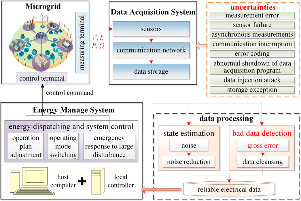
FIGURE 1. Data measuring, transmission, and processing in microgrid.

The electrical data on each Distributed Energy Resource (DER) port, grid port, and load port of the microgrid are collected by the sensors and finally enter the local controller and the host computer via the communication network. These electrical data are used to guide the host computer to issue control commands including the operating mode of each port, input control command value of the converter, and switch on/off command, to realize energy dispatching and system control of the microgrid. However, due to the uncertainties of the data acquisition and communication systems, this electrical data is inevitably mixed with noise and even gross error. In order to improve the reliability of the data, state estimation is needed to reduce noise. At the same time, the bad data detection method is required to clear out the gross error.

2.1 Bad Data in Microgrid

“ An outlier is an observation that deviates so much from other observations as to arouse suspicion that it was generated by a different mechanism” By Douglas M. Hawkins in 1980. The appearance of abnormal data can be seen as a random, sporadic phenomenon relative to the large amount of normal data present, which is largely deviated from normal data and comes from different mechanisms. Therefore, abnormal data often does not have a strong correlation with normal data. This correlation is reflected in two aspects, one is the relevance of the data attribute, the other is the correlation of the data structure. The normal data generally comes from the same mechanism, and the structure is relatively compact, often showing a spherical or band-like structure. The abnormal data does not conform to the intrinsic structure of normal data, and the structural correlation is weak.

According to these characteristics of bad data and normal data, there are two premises in detecting bad data.

Premise 1: Normal data instances occur in dense neighborhoods, while anomalies occur far from their closest neighbors.

Premise 2: Normal data is the majority and is relevant because it arises from the expected mechanism. While abnormal data is generated by sporadic mechanisms and is therefore partially or completely uncorrelated.

Based on the above two premises, the data attributes in the microgrid are shown in Figure 2.

FIGURE 2

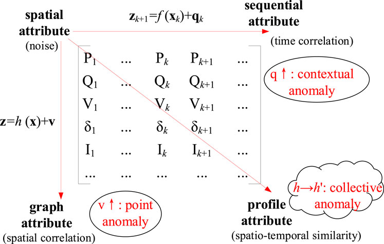
FIGURE 2. Data attribute in microgrid.

We can see from Figure 2 that there are four kinds of attributes of microgrid data, i.e. spatial attribute, graph attribute, sequential attribute, and profile attribute.

1) Spatial attribute refers to different electrical features of the discrete electrical data points formed by the readings of the sensors. As a single data point in the network topology, the data itself contains noise.

2) Graph attribute refers to the neighbor relationship of the sensor in space. At each time interval, the electrical measurements in each column conform to the microgrid measurement equation z = h (x)+v. The electrical data is spatially correlated.

3) Sequential attribute refers to the neighbor relationship of the data sequence in time series. When the topology and parameters of the microgrid keep unchanged, the microgrid is a dynamic time-invariant system. The electrical data sequence z conforms to the state transition equation z_k+1 = f (x_k)+q_k, and the data is also time-dependent.

4) Profile attribute is the scene feature of anomaly defined at the system level in the dimensions of time, space, etc. In the space-time dimension, because different operating scenarios often change periodically, there is a similarity between data sequences.

Based on these four kinds of attributes, three kinds of the anomaly are classified.

1) Point anomaly refers to bad data points in the spatial dimension.

2) Contextual anomaly refers to bad data points or sequences in the time dimension.

3) Collective anomaly refers to abnormal states or patterns in the space-time dimension.

The microgrid bad data discussed in this paper belong to both point anomaly and contextual anomaly, as a result, both spatial correlation and timing correlation can be used to distinguish good data and bad data.

1) bad data in spatial correlation.

The electrical measurements in the microgrid can be expressed as a linear combination of the true values and the measurement errors, as shown in Eq. 1. Note that all the variables are in matrix form.

$\mathbf{z}=h\left(\mathbf{x}\right)+\mathbf{v}(1)$

where $z$ is the measurement, $h\left(x\right)$ is the true value, $x$ is the state variable which ensures the observability of the microgrid, h (·) is the equation expression of the microgrid model, $v$ is the measurement error.

Rewrite Eq. 1 into the time series form.

$\mathbf{z}\left(t\right)=\mathbf{h}\left[x\left(t\right)\right]+\mathbf{v}(2)$

where, t is the time stamp, z(t), x(t), and v are all in vector form.

When $z\left(t\right)$ only contains normal data, the corresponding $v$ stands for the Gaussian white noise.

$\mathbf{v}\sim N\left(\mathbf{0},\mathbf{\sigma }\right)(3)$

where $\sigma$ is the standard deviation of the measurement error $v$.

When $z\left(t\right)$ contains bad data $z_b\left(t\right)$,

$\mathbf{z}\left(t\right)=\left[\begin{array}{c}{\mathbf{z}}_g\left(t\right)\\ {\mathbf{z}}_b\left(t\right)\end{array}\right]=h\left[\mathbf{x}\left(t\right)\right]+\left[\begin{array}{c}{\mathbf{v}}_g\\ {\mathbf{v}}_b\end{array}\right](4)$

where $v_b$ is the gross error, which deviates beyond a certain statistical confidence interval of the normal measurement errors. The confidence interval is usually determined as ±(6–7) $\sigma$ in industrial applications (Clewer Bernard, 1986).

2) bad data in timing correlation.

The microgrid electrical data sequence in time series can also be expressed as

${\mathbf{z}}_{k+1}=f\left({\mathbf{x}}_k\right)+{\mathbf{q}}_k(5)$

where k is the time stamp, f (·) is the equation expression of the microgrid model mapping in time series, and q_k is the surge of electrical measurement.

When q_k, i.e. the difference between the present measured value and the predicted value at the previous sampling time, is very big, there comes an outlier. This outlier may represent bad data. It can also be caused by the sudden change of the microgrid operating state. A further timing correlation method is needed to distinguish the two situations, which will be described later in section 3.

The key to bad data detection lies in the processing of data features. The process is divided into two main steps.

1) Features extraction: the procedure of estimating or predicting the features of bad data. The features include both electrical features and statistical features. The electrical features represent the distance between the measurement $z$ and the true value $h\left(x\right)$. The statistical features represent the distance between the measurement $z$_k+1 in sampling time k+1 and the true value $f\left(x_k\right)$ in sampling time k.

2) Features analysis: using mathematical statistics, data clustering, or other unsupervised methods to approach the interface between normal data and bad data in certain feature dimensions.

The traditional bad data detection method is based on State Estimation.

The diagram of bad data detection based on State Estimation is shown in Figure 3.

FIGURE 3

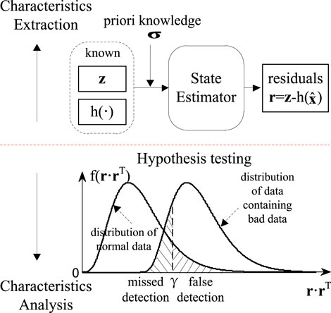
FIGURE 3. Bad data detection based on state estimation.

When the model of the power system can be analytically resolved as expression h (·), the estimated values $\widehat{X}$ of $x$ can be obtained through a State Estimator according to the measurement vector $z$ and the prior knowledge $\sigma$ from the data acquisition system. The electrical features, i.e., residuals $r=z-h\left(\widehat{X}\right)$ are obtained.

Then, the probability distribution f (rr^T) of the residuals r is used as a hypothesis test to detect bad data. The existence of bad data z_b can affect the results of the State Estimation, i.e., residuals r, leading f (rr^T) to change. Therefore, in the vicinity of the boundary where the threshold γ is located, a false or miss detection may occur.

2.2 Bad Data Detection Based on Online Sequential Machine Learning

The electrical features of microgrid measurements have the most abundant prior knowledge for bad data detection. The analytical model $h(\cdot )$ of the microgrid can be approximately fitted as $\widehat{h}(\cdot )$ by supervised online sequential machine learning, as long as plenty of microgrid historical measurements and simulation data (e.g. data from the SIMULINK model of the microgrid in (Beg et al., 2017)) are given. The schematic of the online sequential machine learning based bad data detection is shown in Figure 4.

FIGURE 4

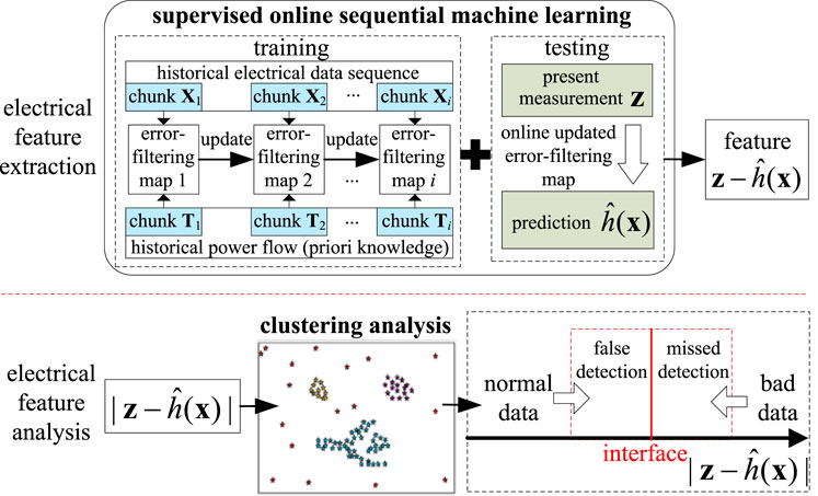
FIGURE 4. Bad data detection based on online sequential machine learning.

Learning from historical data, the online sequential machine learning based bad data detection method constructs an online updating error-filtering map between the historical electrical data sequence and the historical power flow first and then the updated map predicts the true value $\widehat{h}\left(x\right)$ out of the present measurement $z$. Subsequently, the electrical feature $z-\widehat{h}\left(x\right)$ can be obtained.

Since it is hard to discover the statistical properties of the prediction of the machine learning method, the analysis of the feature $z-\widehat{h}\left(x\right)$ cannot be carried out by statistical hypothesis testing. Thus, the unsupervised machine learning method, clustering is used to do the job. Based on the similarity of the data itself, clustering analysis can automatically sort normal data and bad data in different clusters without any prior knowledge. Due to the uncertainty of the boundary between normal data and bad data, a false or missed detection will occur in the vicinity of the interface.

2.3 Bad Data Detection Based on Statistical Analysis in Time Series

Micro-grid is a strong nonlinear time-varying system. Every measurement of the microgrid is not independent but restricted to the electrical mechanism. Therefore, the statistical features of the data in time series indirectly reflect the electrical features and can be used for bad data detection. The schematic of the bad data detection based on the statistical analysis in time series is illustrated in Figure 5.

FIGURE 5

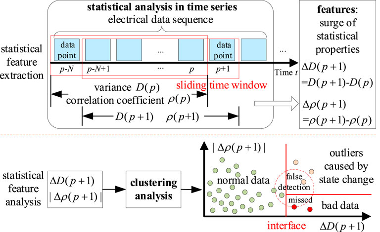
FIGURE 5. Bad data detection based on statistical analysis in time series.

When an outlier (data point p+1) occurs in the microgrid electrical data series, the variance and correlation coefficient of the data sequence in a sliding window with enough width N shows different degrees of the surge. Note that the surge of the variance is $\Delta D\left(p+1\right)$ and the surge of the correlation coefficient is $\Delta \rho \left(p+1\right)$. The $\Delta D\left(p+1\right)$ reflects the continuity of a single-dimensional data sequence, which can be used to recognize outliers. But the outliers can not only be caused by the bad data, but also by the sudden change of the microgrid operating state. When there exists a sudden change of the microgrid operating state, the $\Delta D\left(p+1\right)$ is also significant. Under such a situation, the $\Delta \rho \left(p+1\right)$, reflecting the correlation between the multi-dimensional data sequences, can be used to further distinguish the bad data based on the correlation between different electrical measurements.

Since the operating state of the microgrid changes very often, the threshold of $\Delta D\left(p+1\right)$ and $\Delta \rho \left(p+1\right)$ cannot be determined by a fixed statistical hypothesis testing. So, clustering is used to analyze the two statistical features and sort normal data, outliers, and bad data in different clusters. A false or missed detection can also happen near the boundary of different clusters.

2.4 OSELM Algorithm

A combination of two machine learning algorithms, the supervised ELM and unsupervised DBSCAN, is used for bad data detection in our previous work. Compared to other machine learning algorithms, ELM is well known for its unmatched training speed and great potential for algorithm evolution. Detailed information on ELM and DBSCAN can be referred to (Huang et al., 2018). The OSELM (Liu et al., 2015) which is used in this paper is briefly introduced on the basis of ELM. The network structure and parameters of ELM are shown in Figure A1 in the appendix. Through sequential learning, OSELM can update the machine learning model online, which makes the model more adaptive in the application of time-series data.

3 Sequential Detection via Data-Driven Approach

According to section 2, OSELM is a brand-new online sequential machine learning algorithm that can quickly approximate and update the error-filtering map between the measurements and the true values by recursive linear regression. DBSCAN is very suitable for distinguishing outliers with non-Gaussian distributions, e.g. bad data. Therefore, the combination of OSELM and DBSCAN can quickly realize the sequential detection of the micro-grid bad data. But such a supervised machine learning method, relying on data training, is not sensitive enough to some unfamiliar operating modes or states.

The unsupervised statistical analysis in the time series method, which uses the statistical features (the surge of the variance and the correlation coefficient) in a sliding time window, is proposed to recognize the sudden change of the microgrid operating states.

On this basis, a sequential bad data detection method is proposed by using both the electrical features and the statistical features. The proposed sequential bad data detection method is described as follows. The application details of the proposed statistical analysis in the time series method are explained later.

3.1 Sequential Bad Data Detection

Guided by the previously mentioned two detection ideas, a sequential detection method using a data-driven approach is proposed. It combines the OSELM, the statistical analysis in time series, and the DBSCAN. The flow chart of this method is illustrated in Figure 6.

FIGURE 6

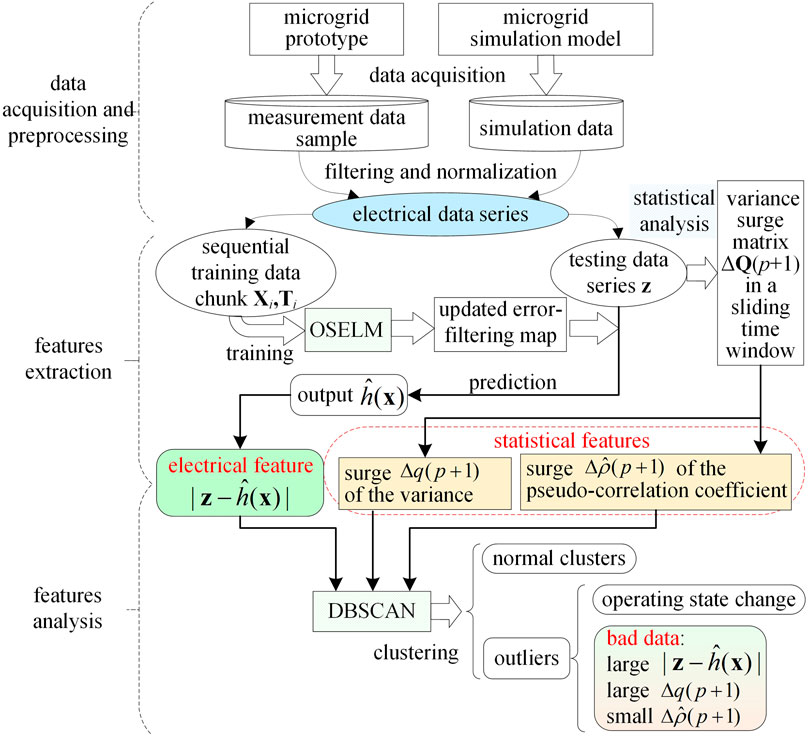
FIGURE 6. Flow chart of the proposed method.

The process of the method is mainly divided into the following steps.

1) Data acquisition and preprocessing.

Collect, screen, and normalize the measurement data of the microgrid prototype and the simulation data of the corresponding microgrid simulation model to form an electrical data series. Next, this processed data series is split into the sequential training data chunks X_i and T_i, (i = 1, 2, … ) and the testing data series $z$. The sequential training data chunks, input matrix X_i come from the old measurement data, and the other sequential training data chunks, target matrix T_i is from the simulation data corresponding to X_i. Meanwhile, the testing data series $z$ is acquired from the current measurement data.

2) Features extraction.

Based on the recursive training method of the OSELM algorithm, the OSELM model is trained by X_i and T_i, (i = 1, 2, … ) to build an online updating error-filtering map. Using the updated error-filtering map to predict the testing data series $z$, the output matrix $\widehat{h}\left(x\right)$ is obtained, and then $\left|z-\widehat{h}\left(x\right)\right|$ is extracted as the electrical feature, i.e. the error (including the gross error) in $z$.

At the same time, the statistical analysis method is developed to calculate the variance surge matrix ∆Q (p+1) of the testing data series $z$ in a sliding time window, where p+1 is the time stamp. The surge of the variance $\Delta q\left(p+1\right)$ and the surge of the pseudo-correlation coefficient $\Delta \widehat{\rho }\left(p+1\right)$ are extracted as the statistical features sequentially.

3) Features analysis.

The aforementioned three features are clustered by DBSCAN to obtain normal clusters and outliers. Outliers with large $\left|z-\widehat{h}\left(x\right)\right|$, large $\Delta q\left(p+1\right)$ , and small $\Delta \widehat{\rho }\left(p+1\right)$ are identified as bad data. The other outliers are recognized as the change of the microgrid operating state.

3.2 Statistical Analysis in Time Series

1) Statistical property of data sequence.

Take the data sequence $z^{M\times N}\left(p\right)$ out of the microgrid measurement matrix $z$ within the fixed time window width N at the pth sampling time. According to Eq. 2, we can see

${\mathbf{z}}^{M\times N}\left(p\right)=\mathbf{h}\left[x\left(t\right)\right]+\mathbf{v}\left(t\right),t=p-N+1,p-N+2,\mathrm{...},p(6)$

where t is the time stamp, M is the dimension of the electrical measurements in $z$.

Calculate the covariance matrix Q(p) of the data sequence $z^{M\times N}\left(p\right)$.

$\mathbf{Q}\left(p\right)=Cov\left({\mathbf{z}}^{M\times N}\left(p\right)\right)=E\left\{\left[{\mathbf{z}}^{M\times N}\left(p\right)\right]{\left[{\mathbf{z}}^{M\times N}\left(p\right)\right]}^T\right\}(7)$

where E is the expectation function.

The entries of matrix Q(p) are

$\begin{array}{l}\{\begin{array}{l}{q}_{ii}\left(p\right)=E{\left[z_i\left(p\right)-{\overline{z}}_i\left(p\right)\right]}^2\\ q_{ij}\left(p\right)=E\left\{\left[z_i\left(t\right)-{\overline{z}}_i\left(p\right)\right]\left[z_j\left(t\right)-{\overline{z}}_j\left(p\right)\right]\right\}\end{array}\\ i,j=\mathrm{1,2},\mathrm{...},M;i\ne j;t=p-N+1,p-N+2,\mathrm{...},p\end{array}(8)$

where $z_i\left(t\right)$ is the ith electrical measurement at sampling time t, ${\overline{z}}_i\left(p\right)$ is the average of the ith electrical measurement sequence over the time window of width N, the diagonal entry $q_{ii}\left(p\right)$ is the variance of the ith electrical measurement in the data sequence at the sampling time p, $q_{ij}\left(p\right)$ is the covariance of the ith electrical measurement and the jth electrical measurement, and $q_{ij}\left(p\right)=q_{ji}\left(p\right)$.

2) Statistical features in sliding time window.

Slide the time window with fixed width N forward by one data point. During this process, the surge of the variance matrix Q is

$\Delta \mathbf{Q}\left(p+1\right)=\mathbf{Q}\left(p+1\right)-\mathbf{Q}\left(p\right)(9)$

The entries of ∆Q (p+1), i.e. the surge of the variance $\Delta q_{ii}\left(p+1\right)$ and covariance $\Delta q_{ij}\left(p+1\right)$ at the (p+1)th sampling time is derived as Eq. 10 under the approximation that ${\overline{z}}_i\left(p+1\right)\approx {\overline{z}}_i\left(p\right)$ (marked as ${\overline{z}}_i$) when N is large enough. At the same time, we assume that the surges before the sampling time (p+1) have been already detected and eliminated. That is to say, $z_i\left(p-N+1\right)\approx {\overline{z}}_i$. Under such conditions, the following equation can be deprived.

$\begin{array}{l}\{\begin{array}{l}\Delta q_{ii}\left(p+1\right)=q_{ii}\left(p+1\right)-q_{ii}\left(p\right)\approx \frac{1}{N}{\left[z_i\left(p+1\right)-{\overline{z}}_i\right]}^2\\ \Delta q_{ij}\left(p+1\right)=q_{ij}\left(p+1\right)-q_{ij}\left(p\right)\approx \frac{1}{N}\left\{\left[z_i\left(p+1\right)-{\overline{z}}_i\right]\left[z_j\left(p+1\right)-{\overline{z}}_j\right]\right\}\end{array}\\ \begin{array}{c}\end{array}i,j=\mathrm{1,2},\mathrm{...},M;i\ne j\end{array}(10)$

According to Eq. 10, if the new arrived electrical measurement $z_i\left(p+1\right)$ is a normal data, it is in the vicinity of ${\overline{z}}_i$, and then $\Delta q_{ii}\left(p+1\right)$ will be quite small. On the contrary, if $z_i\left(p+1\right)$ is an outlier, $\Delta q_{ii}\left(p+1\right)$ is large enough to be defined as a surge. So, $\Delta q_{ii}\left(p+1\right)$ can be used for outlier detection. The outlier may be caused by the bad data. But, it can also be caused by the sudden change of the microgrid operating state. Therefore, the single statistical feature $\Delta q_{ii}\left(p+1\right)$ is not enough for bad data detection.

When the outlier $z_i\left(p+1\right)$ is bad data, the other statistical feature $\Delta q_{ij}\left(p+1\right)$ is also obvious to be defined as a surge. And it is quite smaller than $\Delta q_{ii}\left(p+1\right)$, because $z_j\left(p+1\right)$ is very close to ${\overline{z}}_j$. But, when the outlier $z_i\left(p+1\right)$ is caused by the sudden change of the microgrid operating state, the change of $z_i\left(p+1\right)$ will result in the change of other electrical measurements $z_j\left(p+1\right)$ because they have strong electrical relationships with each other. Thus, some of $z_j\left(p+1\right)$ are much larger than ${\overline{z}}_j$, which makes these $\Delta q_{ij}\left(p+1\right)$ very close to $\Delta q_{ii}\left(p+1\right)$.

Concerning the concept of the correlation coefficient ${\rho }_{ij}\left(p+1\right)=\frac{q_{ij}\left(p+1\right)}{\sqrt{q_{ii}\left(p+1\right)}\sqrt{q_{jj}\left(p+1\right)}}$, we define $\Delta {\widehat{\rho }}_{ij}\left(p+1\right)$ the surge of the pseudo-correlation coefficient as Eq. 11.

$\Delta {\widehat{\rho }}_{ij}\left(p+1\right)=\frac{\Delta q_{ij}\left(p+1\right)}{\Delta q_{ii}\left(p+1\right)}=\frac{z_j\left(p+1\right)-{\overline{z}}_j}{z_i\left(p+1\right)-{\overline{z}}_i},i\ne j(11)$

If the outlier $z_i\left(p+1\right)$ is caused by the bad data, $\Delta {\widehat{\rho }}_{ij}\left(p+1\right)\to 0$. If it is caused by the sudden change of the microgrid operating state, $z_j\left(p+1\right)$ has an electrical relationship with $z_i\left(p+1\right)$, $\left|\Delta {\widehat{\rho }}_{ij}\left(p+1\right)\right|$ ∈[0, 1].

For the application of $\left|\Delta {\widehat{\rho }}_{ij}\left(p+1\right)\right|$, we average it in the dimension j as follows.

$\left|\Delta {\widehat{\rho }}_i\left(p+1\right)\right|=\frac{1}{M-1}{\displaystyle \sum _{j=1,i\ne j}^M\left|\Delta {\widehat{\rho }}_{ij}\left(p+1\right)\right|}(12)$

So, $\left|\Delta {\widehat{\rho }}_{ij}\left(p+1\right)\right|$ can be used as another statistical feature to further distinguish bad data from outliers caused by the sudden change of microgrid operating states.

4 Cases Study

4.1 Acquisition and Preprocessing of Data

The data sequence of the microgrid is obtained from a four-terminal ring-shaped DC microgrid prototype and its simulation model. The topology, control structure, and partial components of the prototype are illustrated respectively in Figures 7–9.

FIGURE 7

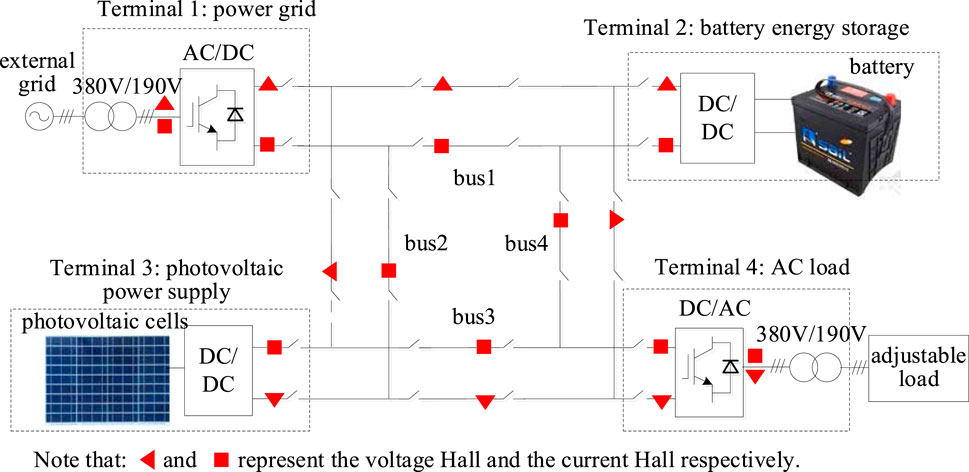
FIGURE 7. Topology of the DC microgrid prototype.

FIGURE 8

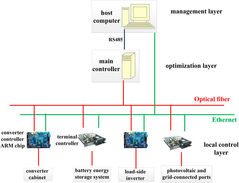
FIGURE 8. Control structure of the DC microgrid prototype.

FIGURE 9

FIGURE 9. Partial components display of the DC microgrid prototype.

According to its control strategy, the microgrid has four operation modes, which are shown in Table 1.

TABLE 1

TABLE 1. Operation modes of the DC microgrid prototype.

There are 24 kinds of electrical measurements collected from the microgrid prototype, namely: terminal voltage and terminal current of the four terminals [U_p1, U_p2, U_p3, U_p4, I_p1, I_p2, I_p3, I_p4], four DC buses voltage [U_dc1, U_dc2, U_dc3, U_dc4], the current flowing through the four positive DC bus [I_dc1, I_dc2, I_dc3, I_dc4], the power output of the four terminals [P₁, P₂, P₃, P₄], the active power and reactive power of the grid side [P_grid, Q_grid], the active power and reactive power of the load side [P_load, Q_load].

The microgrid prototype can be switched between the four operating modes in Table 1 by issuing control commands from the host computer. The data sequence is obtained from the microgrid prototype and its SIMULINK simulation program in the above four control models in a month’s operation. Six sets of testing data were randomly selected. The sampling frequency was 10 Hz, and the sampling time was 13 min 20 s. The Transient processes between different operating modes are removed. The reasons are as follows. First, the physical mechanism of the transient process is clear, rather than caused by uncertainty or unfamiliar mechanisms. Second, the transient process can be detected by the microgrid operation mode switching control signal to know the time of its occurrence, and according to the end of the wide fluctuation of the data to know the time of its end. Therefore, it is not the target of point anomaly detection and contextual anomaly detection in this paper. Each row of the testing data matrix is sorted by electrical quantities order [P₁, P₂, P₃, P₄, P_grid, P_load, Q_grid, Q_load, U_dc1, U_dc2, U_dc3, U_dc4, U_line1, U_line2, U_line3, U_line4, I_dc1, I_dc2, I_dc3, I_dc4, I_line1, I_line2, I_line3, I_line4].

All testing data input and output are scaled, taking the reference value p = 6 kW, Q = 0.5 kVar, U = 550 V, I = 10 A.

4.2 Simulation Cases Design

Parameters Design.

1) The number k of hidden layer nodes in OSELM is set to 80, and the excitation function g (·) is the sigmoid function.

2) The neighborhood radius Eps and the density threshold MinPts of the neighborhood in DBSCAN are set to 0.005 and 4, respectively.

Simulation Environment.

1) The simulation software is MATLAB R2018b.

2) The computer configuration for simulation is core i5 processor with 2.4 GHz frequency plus DDRⅢ memory bank with 8 Gbps memory

4.2.1 Simulation Cases

According to the normal distribution characteristics of the measurement error, the bad data with a gross error of 7–10 times the standard deviation of the measurement error were randomly preset in the six sets of testing data with a content of 5%. The measurement accuracies of the voltage Halls (Type: VSM500D) and the current Halls (Type: LA150-P) used in the micro-grid prototype in the simulation section of this paper are 0.008 and 0.01 respectively. The formula for calculating the standard deviation of errors can be found in reference (Huang et al., 2018).

The bad data preset in this paper includes cases of amplitude jumps (point anomalies), amplitude deviations, and amplitude shifts (contextual anomalies) (Xu et al., 2021). The simulation cases verify the effectiveness of the proposed method by comparing the detection performances of the three algorithms, including the OSELM + DBSCAN method, the ST (statistical analysis) + DBSCAN method, and the OSELM + ST + DBSCAN method. For point anomaly, the detection performance indicators include the right detection rate and calculation time. The right detection rate R_r is calculated by the correct detection times N_r, false detection times N_f, and missed detection times N_m. R_r = N_r/(N_r + N_f + N_m). N_r, N_f, and N_m are confirmed by contrasting the detection results of bad data with the preset location of bad data. For contextual anomaly, the detection performance is quantified by the confusion matrix in Table 2 (Hu et al., 2020; Li et al., 2021a; Li et al., 2021b; Hu et al., 2021; Jung, 2022).

TABLE 2

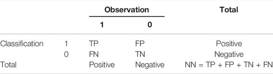
TABLE 2. Confusion matrix.

In Table 2, TP (True Positive) represents true positive events, FN (False Negative) represents false negative events, FP (False Positive) represents false positive events, TN (True Negative) represents true negative events, and NN represents all events. Based on these events, indicators such as Recall (R), Precision (P), Accuracy (Acc), and Error (Err) are chosen to evaluate the detection performance. Their definitions are shown below

$\{\begin{array}{l}R=card\left(\text{TP}\right)/card\left(\text{TP}+\text{FN}\right)\\ P=card\left(\text{TP}\right)/card\left(\text{TP}+\text{FP}\right)\\ Acc=card\left(\text{TP}+\text{TN}\right)/card\left(\text{NN}\right)\\ Err=1-Acc\end{array}(13)$

where card (•) is the counting function. Large values of R, P, and Acc with a small value of Err represent good detection performance.

The OSELM + DBSCAN method, ST + DBSCAN method, and OSELM + ST + DBSCAN method are denoted respectively as methods A, B, and C. The bad data detection results are carried out by using methods A, B, and C for simulation in each case. Each simulation case repeats 10 times, and the average detection performances are calculated.

4.3 Simulation Results and Analysis

1) Case 1: amplitude jumps (point anomaly).

The amplitude jumps are those discrete data points that deviate far from normal data. The detection performances are shown in Table 3.

TABLE 3

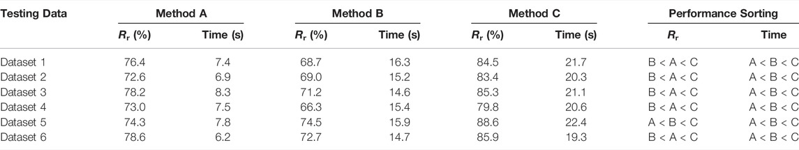
TABLE 3. Detection Performance Comparison between the Three Methods in case 1.

As can be seen from Table 3, for point anomalies, the three methods have good detection results (R_r is between 66% and 89%). Except for Dataset 5, the detection accuracy of Method C is better than that of Method A and Method B, but the calculation time is sacrificed. Relatively speaking, Method B has the worst detection performance.

Randomly select an electrical measurement U_dc2 from Dataset four in Case 1 to visually display the detection effects of the three methods as shown in Figure 10.

FIGURE 10

FIGURE 10. Amplitude jumps detection.

Through Figure 10, it is seen that all three methods can detect point anomaly quite well with a few false detections and missed detections. Method C shows the best performance.

2) Case 2: amplitude deviations (contextual anomaly).

The amplitude deviations are those data sequences that deviate far from normal data series in a stepwise way. The detection performances are shown in Table 4.

TABLE 4

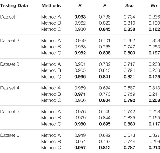
TABLE 4. Detection Performance Comparison between the Three Methods in case 2. The bold values mean the best detection performance among the three detection methods (Method A, Method B, and Method C).

In Table 4, the indicators corresponding to the best detection performance in each dataset are bolded. It can be seen that Method C shows the best performance when detecting the amplitude deviations, except for R in Dataset 1 and Dataset 4.

Randomly select the electrical measurement P₄ from Dataset 1 in Case 2 to visually display the detection effects of the three methods as shown in Figure 11.

FIGURE 11

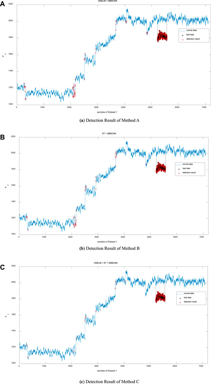
FIGURE 11. Amplitude deviations detection.

Through Figure 11, it is seen that all three methods can detect the amplitude deviation quite well with a few false detections and missed detections. Method C shows the best performance.

3) Case 3: amplitude shifts (contextual anomaly).

The amplitude shifts are those data sequences that slowly shift and continuously deviate from normal data series. The detection performances are shown in Table 5.

TABLE 5

TABLE 5. Detection Performance Comparison between the Three Methods in case 3. The bold values mean the best detection performance among the three detection methods (Method A, Method B, and Method C).

Through Table 5, it can be seen that Method C shows the best performance when detecting the amplitude shifts, except for R and P in Dataset 4.

Randomly select the electrical measurement I_line1 from Dataset 5 in Case 3 to visually display the detection effects of the three methods as shown in Figure 12.

FIGURE 12

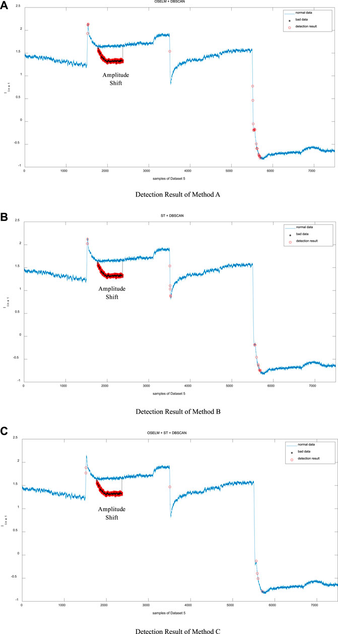
FIGURE 12. Amplitude shifts detection.

Through Figure 12, it is seen that all three methods can detect the amplitude shift quite well with a few false detections and missed detections. Method C shows the best performance.

5 Conclusion

In this paper, the statistical surge feature (ST) is first used for bad data detection, including point anomaly detection and contextual anomaly detection. On this basis, a sequential detection method that combines OSELM, ST, and DBSCAN is proposed for micro-grid bad data detection. The performance of this method is verified by a four-terminal ring-shaped DC micro-grid prototype. By comparing with the existing OSELM + DBSCAN method and the ST + DBSCAN method, it is demonstrated that the proposed OSELM + ST + DBSCAN method has the best detection performance. To be more specific, 1) The OSELM + ST + DBSCAN can detect both point anomaly and contextual anomaly, such as amplitude jumps, amplitude deviations, and amplitude shifts. 2) The OSELM + ST + DBSCAN method can realize the best bad data detection accuracy at the cost of a small increase of computation.

Data Availability Statement

The original contributions presented in the study are included in the article/Supplementary Material, further inquiries can be directed to the corresponding author.

Author Contributions

All authors listed have made a substantial, direct, and intellectual contribution to the work and approved it for publication.

Conflict of Interest

The authors declare that the research was conducted in the absence of any commercial or financial relationships that could be construed as a potential conflict of interest.

Publisher’s Note

All claims expressed in this article are solely those of the authors and do not necessarily represent those of their affiliated organizations, or those of the publisher, the editors and the reviewers. Any product that may be evaluated in this article, or claim that may be made by its manufacturer, is not guaranteed or endorsed by the publisher.

Acknowledgments

The authors would like to thank Professor Andrew Kusiak at the University of Iowa for his academic support on this paper.

Supplementary Material

The Supplementary Material for this article can be found online at: https://www.frontiersin.org/articles/10.3389/fenrg.2022.861563/full#supplementary-material

References

Almalawi, A., Yu, X., Tari, Z., Fahad, A., and Khalil, I. (2014). An Unsupervised Anomaly-Based Detection Approach for Integrity Attacks on SCADA Systems. Comput. Secur. 46, 94–110. doi:10.1016/j.cose.2014.07.005

CrossRef Full Text | Google Scholar

Anwar, A., Mahmood, A. N., and Pickering, M. (2017). Modeling and Performance Evaluation of Stealthy False Data Injection Attacks on Smart Grid in the Presence of Corrupted Measurements. J. Comput. Syst. Sci. 831, 58–72. doi:10.1016/j.jcss.2016.04.005

CrossRef Full Text | Google Scholar

Araya, D. B., Grolinger, K., ElYamany, H. F., Capretz, M. A. M., and Bitsuamlak, G. (2017). An Ensemble Learning Framework for Anomaly Detection in Building Energy Consumption. Energy Build. 144, 191–206. doi:10.1016/j.enbuild.2017.02.058

CrossRef Full Text | Google Scholar

Beg, O., Johnson, T., and Ali, D. (2017). Detection of False-Data Injection Attacks in Cyber-Physical Dc Microgrids. IEEE Trans. Industrial Inf. 13, 2693. doi:10.1109/tii.2017.2656905

CrossRef Full Text | Google Scholar

Bosman, H. H., Iacca, G., Tejada, A., Wörtche, H. J., and Liotta, A. (2017). Spatial Anomaly Detection in Sensor Networks Using Neighborhood Information. Inf. Fusion 33, 41–56. doi:10.1016/j.inffus.2016.04.007

CrossRef Full Text | Google Scholar

Bretas, N. G., and Bretas, A. S. (2015). A Two Steps Procedure in State Estimation Gross Error Detection, Identification, and Correction. Int. J. Electr. Power & Energy Syst. 73, 484–490. doi:10.1016/j.ijepes.2015.05.044

CrossRef Full Text | Google Scholar

Clewer , , and Bernard, C. (1986). State Estimation and Bad Data Detection in Electrical Power System. Diss. Durham University.

Google Scholar

Cramer, M., Goergens, P., and Schnettler, A. (2015). “Bad Data Detection and Handling in Distribution Grid State Estimation Using Artificial Neural Networks,” in 2015 IEEE Eindhoven PowerTech, Eindhoven, Netherlands, 29 June-2 July 2015. doi:10.1109/ptc.2015.7232655

CrossRef Full Text | Google Scholar

Do Coutto Filho, M. B., and de Souza, J. C. S. (2009). Forecasting-Aided State Estimation-Part I: Panorama. IEEE Trans. Power Syst. 24, 1667–1677. doi:10.1109/tpwrs.2009.2030295

CrossRef Full Text | Google Scholar

Gu, W., Lou, G., Tan, W., and Yuan, X. (2017). A Nonlinear State Estimator-Based Decentralized Secondary Voltage Control Scheme for Autonomous Microgrids. IEEE Trans. Power Syst. 32, 4794. doi:10.1109/tpwrs.2017.2676181

CrossRef Full Text | Google Scholar

Hu, X., Huaguang, Z., Dazhong, M., and Rui, W. (2020). A tnGAN-Based Leak Detection Method for Pipeline Network Considering Incomplete Sensor Data. IEEE Trans. Instrum. Meas. 70, 1–10. doi:10.1109/TIM.2020.3045843

PubMed Abstract | CrossRef Full Text | Google Scholar

Hu, X., Zhang, H., Dazhong, M., and Rui, W. (2021). Hierarchical Pressure Data Recovery for Pipeline Network via Generative Adversarial Networks. IEEE Trans. Automation Sci. Eng. 99, 1–11. doi:10.1109/tase.2021.3069003

CrossRef Full Text | Google Scholar

Hu, Y., Kuh, A., Kavcic, A., and Nakafuji, D. (2011). “Real-time State Estimation on Micro-grids,” in The 2011 International Joint Conference on Neural Networks, San Jose, CA, USA, 31 July-5 Aug. 2011. doi:10.1109/ijcnn.2011.6033385

CrossRef Full Text | Google Scholar

Huang, H., Liu, F., Zha, X., Xiong, X., Ouyang, T., Liu, W., et al. (2018). Robust Bad Data Detection Method for Microgrid Using Improved ELM and DBSCAN Algorithm. J. Energy Eng. 144, 04018026. doi:10.1061/(asce)ey.1943-7897.0000544

CrossRef Full Text | Google Scholar

Huang, S.-J., and Lin, J.-M. (2004). Enhancement of Anomalous Data Mining in Power System Predicting-Aided State Estimation. IEEE Trans. Power Syst. 19, 610–619. doi:10.1109/tpwrs.2003.818726

CrossRef Full Text | Google Scholar

Huang, Y., Tang, J., Cheng, Y., Li, H., Campbell, K. A., and Han, Z. (2016). Real-time Detection of False Data Injection in Smart Grid Networks: an Adaptive CUSUM Method and Analysis. IEEE Syst. J. 10, 532–543. doi:10.1109/jsyst.2014.2323266

CrossRef Full Text | Google Scholar

Jung, A. (2022). Machine Learning: The Basics. Singapore: Springer. Available at: http://mlbook.cs.aalto.fi.

Google Scholar

Li, H., Deng, J., Feng, P., Pu, C., Arachchige, D. K., and Cheng, Q. (2021). Short-Term Nacelle Orientation Forecasting Using Bilinear Transformation and ICEEMDAN Framework. Front. Energy Res. 9, 780928. doi:10.3389/fenrg.2021.780928

CrossRef Full Text | Google Scholar

Li, H., Deng, J., Yuan, S., Feng, P., and Arachchige, D. K. (2021). Monitoring and Identifying Wind Turbine Generator Bearing Faults Using Deep Belief Network and EWMA Control Charts. Front. Energy Res. 9, 799039. doi:10.3389/fenrg.2021.799039

CrossRef Full Text | Google Scholar

Li, S., Yilmaz, Y., and Wang, X. (2015). Quickest Detection of False Data Injection Attack in Wide-Area Smart Grids. IEEE Trans. Smart Grid 6, 2725–2735. doi:10.1109/tsg.2014.2374577

CrossRef Full Text | Google Scholar

Liu, Y., He, B., Dong, D., Shen, Y., Yan, T., Nian, R., et al. (2015). “ROS-ELM: A Robust Online Sequential Extreme Learning Machine for Big Data Analytics,” in Proceedings of ELM-2014 (Cham: Springer International Publishing), 325–344.

CrossRef Full Text | Google Scholar

Liu, Y., Ning, P., and Reiter, M. K. (2011). False Data Injection Attacks against State Estimation in Electric Power Grids. ACM Trans. Inf. Syst. Secur. (TISSEC) 14, 13. doi:10.1145/1952982.1952995

CrossRef Full Text | Google Scholar

Mohammadpourfard, M., Sami, A., and Seifi, A. R. (2017). A Statistical Unsupervised Method against False Data Injection Attacks: A Visualization-Based Approach. Expert Syst. Appl. 84, 242–261. doi:10.1016/j.eswa.2017.05.013

CrossRef Full Text | Google Scholar

Qiu, R., Lei, C., Xing, H., Zenan, L., and Haichun, L. (2017). Spatio-Temporal Big Data Analysis for Smart Grids Based on Random Matrix Theory: A Comprehensive Study. Ithaca, NY: arXiv preprint of Cornell University. arXiv preprint arXiv:1708.04935.

Google Scholar

Rana, M., Li, L., and Li, Li. (2015). An Overview of Distributed Microgrid State Estimation and Control for Smart Grids. Sensors 15, 4302–4325. doi:10.3390/s150204302

PubMed Abstract | CrossRef Full Text | Google Scholar

Rana, M. M., and Li., L. (2015). Microgrid State Estimation and Control for Smart Grid and Internet of Things Communication Network. Electron. Lett. 512, 149–151. doi:10.1049/el.2014.3635

CrossRef Full Text | Google Scholar

Ren, H., Liu, M., Li, Z., and Pedrycz, W. (2017). A Piecewise Aggregate Pattern Representation Approach for Anomaly Detection in Time Series. Knowledge-Based Syst. 135, 29–39. doi:10.1016/j.knosys.2017.07.021

CrossRef Full Text | Google Scholar

Shahnia, F., Majumder, R., Ghosh, A., Ledwich, G., and Zare, F. (2010). Operation and Control of a Hybrid Microgrid Containing Unbalanced and Nonlinear Loads. Electr. Power Syst. Res. 808, 954–965. doi:10.1016/j.epsr.2010.01.005

CrossRef Full Text | Google Scholar

Shyh-Jier, H., and Jeu-Min, L. (2002). Enhancement of Power System Data Debugging Using GSA-Based Data-Mining Technique. IEEE Trans. Power Syst. 17, 1022–1029. doi:10.1109/tpwrs.2002.804992

CrossRef Full Text | Google Scholar

Wu, Y., Onwuachumba, A., and Musavi, M. (2013). “Bad Data Detection and Identification Using Neural Network-Based Reduced Model State Estimator,” in 2013 IEEE Green Technologies Conference (GreenTech), Denver, CO, USA, 4-5 April 2013. doi:10.1109/greentech.2013.35

CrossRef Full Text | Google Scholar

Wu, Y., Xiao, Y., Hohn, F., Nordstorm, L., Wang, J., and Zhao, W. (2017). Bad Data Detection Using Linear WLS and Sampled Values in Digital Substations. IEEE Trans. Power Deliv. 99, 1–8. doi:10.1109/TPWRD.2017.2669110

CrossRef Full Text | Google Scholar

Xia, N., Gooi, H. B., Chen, S., and Hu, W. (2016). Decentralized State Estimation for Hybrid AC/DC Microgrids. IEEE Syst. J. 12, 434. doi:10.1109/JSYST.2016.2615428

CrossRef Full Text | Google Scholar

Xu, F., Xue, A., Chang, N., Kong, H., and Xu, J. (2021). Research Status and Prospects of Detection, Correction and Recovery for Abnormal Synchrophasor Data in Power System. Proc. CSEE 41 (20), 6869–6886. doi:10.13334/j.0258-8013.pcsee.202180

CrossRef Full Text | Google Scholar

Yang, L., Li, Y., and Li, Z. (2017). Improved-ELM Method for Detecting False Data Attack in Smart Grid. Int. J. Electr. Power & Energy Syst. 91, 183–191. doi:10.1016/j.ijepes.2017.03.011

CrossRef Full Text | Google Scholar

Zhao, J., Liu, K., Wang, W., and Liu, Y. (2014). Adaptive Fuzzy Clustering Based Anomaly Data Detection in Energy System of Steel Industry. Inf. Sci. 259, 335–345. doi:10.1016/j.ins.2013.05.018

CrossRef Full Text | Google Scholar

Zhao, J., Zhang, G., Scala, M. L., and Wang, Z. (2017). Enhanced Robustness of State Estimator to Bad Data Processing through Multi-Innovation Analysis. IEEE Trans. Ind. Inf. 134, 1610–1619. doi:10.1109/tii.2016.2626782

CrossRef Full Text | Google Scholar