Grey Wolf Optimization–Based Deep Echo State Network for Time Series Prediction

The Echo State Network (ESN) is a unique type of recurrent neural network. It is built atop a reservoir, which is a sparse, random, and enormous hidden infrastructure. ESN has been successful in dealing with a variety of non-linear issues, including prediction and classification. ESN is utilized in a variety of architectures, including the recently proposed Multi-Layer (ML) architecture. Furthermore, Deep Echo State Network (DeepESN) models, which are multi-layer ESN models, have recently been proved to be successful at predicting high-dimensional complicated non-linear processes. The proper configuration of DeepESN architectures and training parameters is a time-consuming and difficult undertaking. To achieve the lowest learning error, a variety of parameters (hidden neurons, input scaling, the number of layers, and spectral radius) are carefully adjusted. However, the optimum training results may not be guaranteed by this haphazardly created work. The grey wolf optimization (GWO) algorithm is introduced in this study to address these concerns. The DeepESN based on GWO (GWODESN) is utilized in trials to forecast time series, and therefore the results are compared with the regular ESN, LSTM, and ELM models. The findings indicate that the planned model performs the best in terms of prediction.

1 Introduction

Time series appear in every facet of life, and one of the current research topics is time series forecasting. Time series prediction may be aided by the development of new methodologies. The time series, on the other hand, is frequently created by a chaotic system and is untidy or non-linear. As a result, time-series forecasting research is extremely difficult. Furthermore, time series prediction requires models with high prediction accuracy.

Over the two past decades, several researchers proposed various models for time series forecasting that involve scientific prediction based on historical time-stamped data. Among these researchers, Liu (2017) presented a time-series prediction approach based on an online sequential extreme learning machine (OS-ELM). This approach was later updated to include an adaptive forgetting factor and a bootstrap to improve the prediction accuracy and stability. Guo et al. (2016) used differential evolution (DE) to optimize the model parameters in an efficient extreme learning machine (EELM) that is utilized to anticipate chaotic time series. Lukoseviciute et al. (2018) used evolutionary algorithms and Bernstein polynomials to develop a short-term time-series prediction model. For chaotic time series, Ma et al. (2004) suggested a mixed model based on neural networks and wavelets. Milad et al. (2017) proposed a model of adaptive decayed brain emotional learning (ADBEL) to better handle online forecasting of time series through a neuro-fuzzy network architecture. Miranian and Abdollahzade (2013) proposed a local neuro-fuzzy (LNF) scheme combined with least-square support vector machines (LSSVMs) for non-linear and chaotic modeling and forecasting. Tang et al. (2020) proposed a LSSVM model to model NOx emissions. Chai and Lim (2016) constructed a discriminative model of a neural network architecture equipped with weighted fuzzy membership functions (NEWFM) for identifying patterns of economic time series. Li et al. (2016) proposed an adaptive Volterra-type prediction model with matrix factorization for chaotic time-series analysis. Su and Yang (2021) proposed a brain emotional network in conjunction with an adaptive genetic algorithm (BEN-AGA) model for predicting time series of chaotic behavior. Nevertheless, the aforementioned methods have several limitations. First, an adequate structure must be pre-specified for the conventional neural networks, and the convergence rate of these networks is slow. Also, the ELM method exhibits weak generalization and robustness. Also, the LSSVM method is greatly affected by time delays.

Recently, recurrent neural networks (RNNs) have been introduced to handle problems with temporal dynamics. The RNN architectures have been successfully utilized for time-series detection (Li et al., 2021a) and forecasting (Li et al., 2021b). However, the overall RNN weights should be learned through backpropagation, and this imposes a significant computational burden. To enhance the operational efficiency, Echo State Networks (ESNs) were proposed by Jaeger and Haas (2004) as a novel RNN variant that can be efficiently utilized for time series forecasting. For example, Han et al. (2021) proposed an optimized ESN model with adaptive error compensation for network traffic prediction. Liu et al. (2020) proposed a hybrid time-series prediction approach with the binary grey wolf algorithm and echo state networks (BGWO-ESN). Beyond time series forecasting, the echo state networks have also been applied in other problems, including mainly classification (Stefenon et al., 2022), detection (Steiner et al., 2021), and image segmentation (Abdelkerim et al., 2020). However, the conventional ESN architectures still lack the ability to handle complicated tasks. To address this limitation, a DeepESN model is introduced in this paper, where a grey wolf optimization (GWO) algorithm is used to optimize the DeepESN model parameters. Our proposed DeepESN architecture is evaluated on the Lorenz system, the Mackey–Glass (MG) model, and the non-linear autoregressive moving average (NARMA) model. The proposed method was evaluated with a real-time series representing full-load electrical power outputs. The simulations demonstrate promising performance of the proposed forecasting strategy.

The main contributions of this paper are highlighted as follows: first, the effort made in the paper represents one of the first few attempts to construct DeepESN to forecast times series. Then, compared with ESN, LSTM, and ELM models, the proposed GWODESN outperforms in terms of forecast accuracy.

The remainder of this work is arranged as follows. A detailed overview of the DeepESN and GWO algorithms is presented in Section 2, while Section 3 provides the details of the proposed GWODESN model. The simulation outcomes are analyzed in Section 4. Then, Section 5 gives final conclusions.

2 Methodology

2.1 Deep Echo State Networks

Following the conventional ESN model, the DeepESN model is made up of multiple dynamical reservoir components. Specifically, the DeepESN reservoir is organized into stacked repetitive layers. For each layer, the output is the input of the next layer, as outlined in Figure 1 (Gallicchio and Micheli, 2017). In our work, NU indicates the number of the input measurements, NL indicates the reservoir layer count, NR denotes the number of the recurrent units, and t indicates time. Moreover, u(t) denotes the model input at time t, whereas x⁽ⁱ⁾(t) represents the state for the ith reservoir layer at time t. The DeepESN reservoir dynamics are mathematically modeled as follows. The dynamics of the primary DeepESN layer can be expressed as

${\text{x}}^{\left(1\right)}\left(t\right)=(\text{1}-{\mathrm{a}}^{\left(1\right)}){\mathrm{x}}^{\left(1\right)}(t-1)+{\mathrm{a}}^{\left(1\right)}\mathrm{f}({\mathrm{W}}^{\left(1\right)}\mathrm{ u}\left(t\right)+{\widehat{\mathrm{W}}}^{\left(1\right)}{\mathrm{x}}^{\left(1\right)}(t-1))(1)$

FIGURE 1

FIGURE 1. Architecture of a DeepESN.

When i > 1, the DeepESN state is computed as

${\mathrm{x}}^{\left(i\right)}\left(t\right)=(\text{1}-{\mathrm{a}}^{\left(i\right)}){\mathrm{x}}^{\left(i\right)}(t-1)+{\mathrm{a}}^{\left(i\right)}\mathrm{f}({\mathrm{W}}^{\left(i\right)}{\text{ x}}^{\left(i\right)}\left(t\right)+{\widehat{\mathrm{W}}}^{\left(i\right)}{\mathrm{x}}^{\left(i\right)}(t-1))(2)$

where W⁽¹⁾ indicates the input weight matrix, W⁽ⁱ⁾ indicates the weights of the connections between the (i − 1)^th and ith layers, ${\widehat{\text{W}}}^{\left(i\right)}$ indicates the recurrent weights of the ith layer, a ⁽ⁱ⁾ ∈ [0, 1] indicates the leakage rate of the ith layer, and f represents the employed activation function (regularly chosen as the tanh function).

2.2 Grey Wolf Optimizer

GWO could be a nature-inspired algorithm that imitates the chain of command of administration and daily routine (Mirjalili et al., 2014). The wolves have four conceivable sorts: alpha, beta, delta, or omega. The pioneers of the pack (called alphas), which may be recognized by the leading administration abilities instead of the most grounded body, make choices almost every day exercises for the whole pack. The beta wolf helps alpha to make a choice. The omega wolf position is most reduced among wolves, but it plays a key part in keeping up a prevailing structure. The delta wolf is auxiliary to the alpha and beta, but it has the upper hand over the omega within the previously mentioned chain of command. The GWO algorithm can be mathematically represented as follows:

$\overrightarrow{D}=\left|C\cdot \overrightarrow{X_p}\left(t\right)-\overrightarrow{X}\left(t\right)\right|(3)$

$\overrightarrow{X}(t+1)=\overrightarrow{X_p}\left(t\right)-A\cdot \overrightarrow{D}(4)$

where t is utilized to mean the current iteration, $\overrightarrow{X_p}$ to mean the prey position vector, and $\overrightarrow{X}$ to represent the wolf position vector. Meanwhile, A and C can be represented as

$A=2a\cdot r_1-a(5)$

$C=2\cdot r_2(6)$

where a is diminished in a straight design from 2 to 0. r₁, r₂ are haphazardly created from the unit interval [0,1]. The wolf pack chasing design is driven by the alpha wolves and frequently by the beta and delta ones. This design may be scientifically sculptural as takes after

$\begin{array}{l}\overrightarrow{D_{\alpha }}=|C_1\cdot \overrightarrow{X_{\alpha }}-\overrightarrow{X}|\\ \overrightarrow{D_{\beta }}=|C_2\cdot \overrightarrow{X_{\beta }}-\overrightarrow{X}|\\ \overrightarrow{D_{\delta }}=|C_3\cdot \overrightarrow{X_{\delta }}-\overrightarrow{X}|\end{array}(7)$

$\begin{array}{l}\overrightarrow{X_1}=\overrightarrow{X_{\alpha }}-A_1\cdot \overrightarrow{D_{\alpha }}\\ \overrightarrow{X_2}=\overrightarrow{X_{\beta }}-A_2\cdot \overrightarrow{D_{\beta }}\\ \overrightarrow{X_3}=\overrightarrow{X_{\delta }}-A_3\cdot \overrightarrow{D_{\delta }}\end{array}(8)$

$\overrightarrow{X}(t+1)=(\overrightarrow{X_1}+\overrightarrow{X_2}+\overrightarrow{X_3})/3(9)$

3 Grey Wolf Optimizer–Based Deep Echo State Network

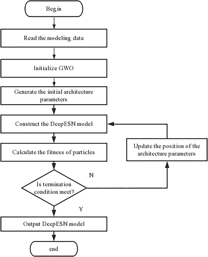
As the same as simple ESN model, we must appropriately indicate network parameters of DeepESN for getting palatable comes about. We might rehash the tests trusting to secure great plan scenarios. Be that as it may, we can never be sure that the best solution has been achieved. To address it, the GWO algorithm ought to be utilized to optimize a couple of parameters including NR, NL, ρ, and IR. The spectral radius ρ is one in all the foremost central parameters characterizing the reservoir’s weight matrix W. And to take care of the echo state property (ESP), ρ should be scaled to equal or less than one. Figure 2 shows a flowchart of the proposed GWODESN. The taking after steps depict the particular modeling strategy:

FIGURE 2

FIGURE 2. A flowchart of the proposed modeling approach.

Step 1Read time series file as the input data.

Step 2Initialize the GWO algorithm containing the a, A, and C.

Step 3Set initial population representing NR, NL, ρ, and IR.

Step 4Use initial population to establish the DeepESN model.

Step 5Calculate the mean absolute error of various population as the corresponding fitness value.

Step 6Obtain initial optimum value having least fitness values in population.

Step 7If the fitness value obtained meets the accuracy requirements of the model, skip to Step 9. Something else, proceed.

Step 8Update the population applying Eq. 9, the number of iterations t = t+1, and then return to Step 4.

Step 9Output the best NR, NL, ρ, and IR.

4 Experimental Setup, Results, and Discussion

In this pondering, three benchmark datasets and one real-world illustration are embraced to confirm the execution of diverse models. One-step ahead expectation is examined in this segment. To assess the created demonstration, 4 standard records (Tang et al., 2020; Li et al., 2021a; Li et al., 2021b) including the mean absolute error (MAE), the mean absolute percentage error (MAPE), the root-mean-square error (RMSE), and the coefficient of determination (R²) are characterized as takes after

$MAE=\frac{1}{M}{\displaystyle \sum _{j=1}^M\left|y_j-{\widehat{y}}_j\right|}(10)$

$MAPE=\frac{1}{M}{\displaystyle \sum _{j=1}^M\frac{\left|y_j-{\widehat{y}}_j\right|}{y_j}}(11)$

$RMSE=\sqrt{\frac{1}{M}{\displaystyle \sum _{j=1}^M{(y_j-{\widehat{y}}_j)}^2}}(12)$

$R^2=1-\frac{{\displaystyle \sum _{j=1}^M{(y_j-{\widehat{y}}_j)}^2}}{{\displaystyle \sum _{j=1}^M{(y_j-{\overline{y}}_j)}^2}}(13)$

Within the equations, M is utilized to represent sample size, $y_j$ to represent the true value, ${\overline{y}}_j$ to represent mean true value, and ${\widehat{y}}_j$ to represent the forecast value. All experiments were carried out in MATLAB on a Windows 10 operating system, with a 2.50-GHz Intel CPU, and a memory of 8.0 GB. The performance outcomes of our approach were compared with those based on the conventional ESN, ELM, and LSTM architectures.

4.1 Lorenz System

The Lorenz dynamical system (Wu et al., 2021) is a key benchmark of time series forecasting and is mathematically defined as

$\begin{array}{l}\frac{dx}{dt}=a(-x+y)\\ \frac{dy}{dt}=bx-y-xz\\ \frac{dz}{dt}=xy-cz\end{array}(14)$

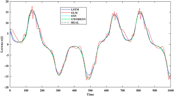
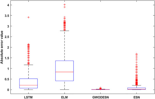
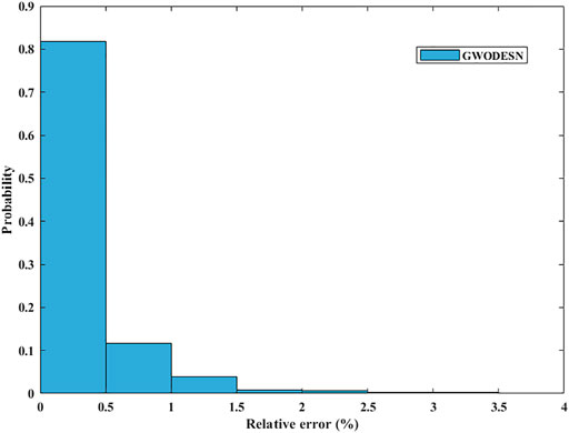
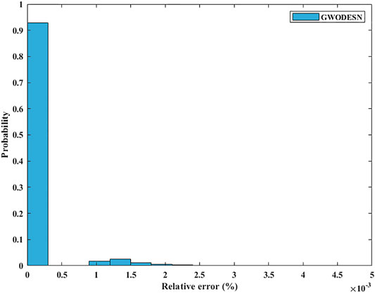
where t expresses time, while the model coefficients a, b, and c are respectively chosen as 10, 28, and 8/3. Model training and testing were carried out with time series lengths of 4,000 and 1,000, respectively. For x-dimensional forecasting, past information of x(t −1), y(t −1), and z(t −1) is utilized in the prediction of the present x(t) values. In the arrangement to assess the viability and preferences of this proposed GWODESN, the conventional ESN, ELM, and the LSTM are chosen as benchmarks. The real value and the anticipated value of GWODESN, ESN, ELM, and the LSTM to begin with appeared in Figure 3, and the expectation exactness is recorded in Table 1. It is clear that GWODESN is superior than others, showing the adequacy of this approach. In expansion, the yield of ELM cannot coordinate the real esteem, particularly at a few emphasis focuses. It moreover outlines the justification of RNN. The expectation mistakes of GWODESN, ESN, ELM, and the LSTM are advance compared in Figure 4. Figure 4 shows the box graph of absolute error recorded for 30 runs of diverse models. It can be seen that the GWODESN shows superior forecast exactness and solidness than other models. The absolute error box graph of the ELM demonstration is long, and it is known that the supreme mistake values are scattered, showing that the forecast performance of the ELM model is not as steady as in other models. The box chart of the GWODESN model is the most brief. Most of the absolute error values are smaller than other comparison models. Figure 5 gives the relative error distribution of the testing information by the GWODESN. Among the 1,000 testing cases, 93.3% of the relative errors were less than 1%. In general, the prediction accuracy of the GWODESN model is relatively high and relatively stable. In common, the expectation precision of the GWODESN model is moderately high and generally steady.

FIGURE 3

FIGURE 3. The real value and the anticipated value for Lorenz x(t).

TABLE 1

TABLE 1. The performance comparison of GWODESN, ESN, ELM, and the LSTM for Lorenz x(t)

FIGURE 4

FIGURE 4. The absolute error box diagram for Lorenz x(t).

FIGURE 5

FIGURE 5. Relative error distribution for Lorenz x(t).

4.2 NARMA system

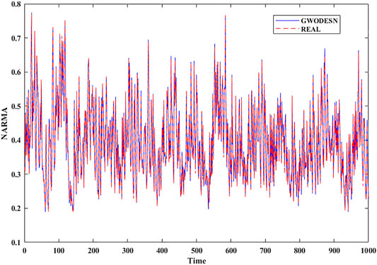
NARMA (Chouikhi et al., 2017), which is featured with a very high rate of chaos in its behavior, could also be an accepted studied benchmark. The flow of this benchmark is produced by Eq. 15:

$y(t+1)=c_{1}y\left(t\right)+c_{2}y\left(t\right){\displaystyle \sum _{i=1}^{k}y(t-i)}+c_{3}x(t-(k-1))x\left(t\right)+c_4(15)$

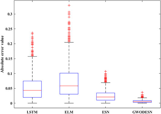
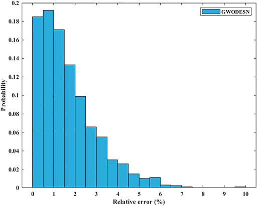
where y(t) and x(t) are the yield and input of the framework at time t, separately. The consistent c is set as 0.3, 0.05, 1.5, and 0.1, separately. The k, which decides the intricacy of NARMA, is set to 10. As the same as the past simulation, the real value and the anticipated value of GWODESN are shown in Figure 6, and the desired precision is recorded in Table 2. It is evident that GWODESN can take after the real esteem ideally. The desired botches of GWODESN, ESN, ELM, and the LSTM are developed and compared in Figure 7. It can be seen in Figure 7 that the GWODESN appears to have a more predominant estimate precision and solidness than other models. The absolute error box graph of the ELM is long, and it is known that the incomparable botch values are scattered, appearing that the figure execution of the ELM is not as steady as other models. The box chart of the GWODESN show is the foremost brief. Most of the absolute error values are more diminutive than other comparison models. Figure 8 gives the relative error dispersion of the testing data by the GWODESN. Among the 1,000 testing cases, 90.1% of the relative error distribution were less than 3.5% as appeared in Figure 8.

FIGURE 6

FIGURE 6. The real value and the anticipated value for NARMA.

TABLE 2

TABLE 2. Prediction performance comparison for NARMA

FIGURE 7

FIGURE 7. The absolute error box diagram for NARMA.

FIGURE 8

FIGURE 8. Relative error distribution for NARMA.

4.3 Mackey–Glass System

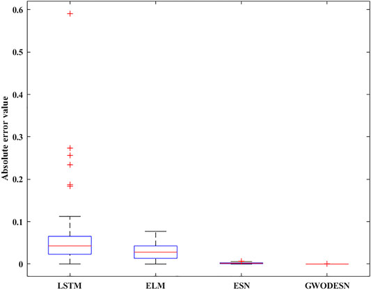
The MG (Mackey and Glass, 1977) may be a normal chaotic framework, which is known by its non-linear behavior. Thus, learning the designs appears to be a troublesome errand. It is portrayed by Eq. 16.

$\frac{dx\left(t\right)}{dt}=\frac{0.\mathrm{2}x(t-\tau )}{\mathit{1}+{{\displaystyle x}}^{10}(t-\tau )}-\mathit{0}.\mathit{1}x\left(t\right)(16)$

where $\tau$ is a vital parameter of the MG system, which is regularly set to 17. In total, 4,000 tests were utilized as training data sets and 1,000 tests were utilized for testing. The forecast that comes about appears in Figure 9 and Table 3. The conventional utilized ESN can be seen to have superior forecast execution than the ELM and the LSTM and can fit the original data well. Be that as it may, the execution of the GWODESN is superior than that of the conventional ESN. Figure 10 appears that the GWODESN show has superior forecast precision and soundness than other models. Among the 1,000 testing cases, 99% of the relative mistakes were less than 1% in Figure 11.

FIGURE 9

FIGURE 9. The real value and the anticipated value for MG.

TABLE 3

TABLE 3. Prediction performance comparison for MG

FIGURE 10

FIGURE 10. The absolute error box diagram for MG.

FIGURE 11

FIGURE 11. Relative error distribution for MG.

4.4 Combined Cycle Power Plants

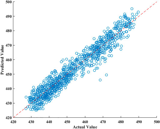
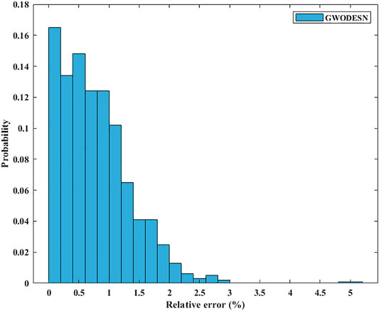
CCPPs generally contain steam turbines (STs) and gas turbines (GTs), as well as heat recovery steam generators (HRSGs). For a CCPP, power generation is jointly performed by the steam and gas turbines, and is exchanged between each turbine and the others (Tüfekci, 2014). Here, we use CCPP data to evaluate the single-step prediction performance. The utilized dataset includes four input factors and one target variable, where this dataset was collected from 2006 to 2011. Figure 12 outlines both the GWODESN-predicted and measured electrical power outputs. The specked reddish straight line represents the ideal relationship of the predicted and measured values. The blue line demonstrates the GWODESN predicted outcomes. Almost all of the predictions are scattered around the ideal line. Figure 13 gives the relative error distribution of the GWODESN model on the test data. Among the 1,000 test samples, 90.3% of the relative errors are less than 1.6%. Obviously, the GWODESN model outperforms the other three competing models. The adequacy of the proposed model is shown by the results in Table 4.

FIGURE 12

FIGURE 12. Scatter diagram of the real value and the anticipated value for CCPP.

FIGURE 13

FIGURE 13. Relative error distribution for CCPP.

TABLE 4

TABLE 4. Prediction performance comparison for CCPP

5 Conclusion

In this paper, the GWODESN is created for time series expectation. The four primary parameters of the DESN were optimized by utilizing the GWO algorithm. Four ordinary time series, counting Lorenz, MG, NARMA, and CCPP, are chosen as the simulation objects. Comparative test that comes about on four time-series forecast assignments clearly illustrates that the proposed GWODESN outflank the ELM, LSTM, and ESN benchmarks. The expectation strategy is basic and effective, and has certain hypothetical centrality and commonsense esteem. Hyper-parameter optimization and the topology of the networks are all the common optimization strategies. Within the future, we will center on progressing the network topology and apply the model in other domains, such as wind energy prediction.

Data Availability Statement

The raw data supporting the conclusion of this article will be made available by the authors, without undue reservation.

Author Contributions

XC designed the research and the article structure, and revised the article. HZ carried out the experiments and revised the article.

Conflict of Interest

The authors declare that the research was conducted in the absence of any commercial or financial relationships that could be construed as a potential conflict of interest.

Publisher’s Note

All claims expressed in this article are solely those of the authors and do not necessarily represent those of their affiliated organizations, or those of the publisher, the editors and the reviewers. Any product that may be evaluated in this article, or claim that may be made by its manufacturer, is not guaranteed or endorsed by the publisher.

References

Abdelkerim, S., Amma, B., Zoubir, A. F., and Elhadj, B. H. (2020). Echo State Network‐based Feature Extraction for Efficient Color Image Segmentation. J. Concurrency Computation: Pract. Experience 32 (21), 1. doi:10.1002/cpe.5719

CrossRef Full Text | Google Scholar

Chai, S. H., and Lim, J. S. (2016). Forecasting Business Cycle with Chaotic Time Series Based on Neural Network with Weighted Fuzzy Membership Functions. Chaos, Solitons & Fractals 90 (1), 118–126. doi:10.1016/j.chaos.2016.03.037

CrossRef Full Text | Google Scholar

Chouikhi, N., Ammar, B., Rokbani, N., and Alimi, A. M. (2017). PSO-based Analysis of echo State Network Parameters for Time Series Forecasting. Appl. Soft Comput. 55, 211–225. doi:10.1016/j.asoc.2017.01.049

CrossRef Full Text | Google Scholar

Gallicchio, C., and Micheli, A. (2017). Deep Echo State Network (DeepESN): A Brief Survey Statistics, 1–15.

Google Scholar

Guo, W., Xu, T., and Lu, Z. (2016). An Integrated Chaotic Time Series Prediction Model Based on Efficient Extreme Learning Machine and Differential Evolution. Neural Comput. Applic 27 (4), 883–898. doi:10.1007/s00521-015-1903-2

CrossRef Full Text | Google Scholar

Han, Y., Jing, Y. W., Dimirovski, G. M., and Zhang, L. (2021). Multi-step Network Traffic Prediction Using echo State Network with a Selective Error Compensation Strategy [J]. Transactions of the Institute of Measurement & Control, 1. doi:10.1177/01423312211050296

CrossRef Full Text | Google Scholar

Jaeger, H., and Haas, H. (2004). Harnessing Nonlinearity: Predicting Chaotic Systems and Saving Energy in Wireless Communication. science 304 (5667), 78–80. doi:10.1126/science.1091277

PubMed Abstract | CrossRef Full Text | Google Scholar

Li, H., Deng, J., Feng, P., Pu, C., Arachchige, D. D., and Cheng, Q. (2021). Short-Term Nacelle Orientation Forecasting Using Bilinear Transformation and ICEEMDAN Framework. Front. Energ. Res. 9, 1–14. doi:10.3389/fenrg.2021.780928

CrossRef Full Text | Google Scholar

Li, H., Deng, J., Yuan, S., Feng, P., and Arachchige, D. D. (2021). Monitoring and Identifying Wind Turbine Generator Bearing Faults Using Deep Belief Network and EWMA Control Charts. Front. Energ. Res. 9, 1–10. doi:10.3389/fenrg.2021.799039

CrossRef Full Text | Google Scholar

Li, Y., Zhang, Y., Wang, J., Huang, B., and Liu, W. (2016). The Volterra Adaptive Prediction Method Based on Matrix Decomposition. J. Interdiscip. Maths. 19 (2), 363–377. doi:10.1080/09720502.2015.1113692

CrossRef Full Text | Google Scholar

Liu, J. Z. (2017). Adaptive Forgetting Factor OS-ELM and Bootstrap for Time Series Prediction. Int. J. Model. Simulation, Scientific Comput. [J] 8 (3), 1–19. doi:10.1142/s1793962317500295

CrossRef Full Text | Google Scholar

Liu, J., Sun, T., Luo, Y., Yang, S., Cao, Y., and Zhai, J. (2020). Echo State Network Optimization Using Binary Grey Wolf Algorithm. Neurocomputing 385, 310–318. doi:10.1016/j.neucom.2019.12.069

CrossRef Full Text | Google Scholar

Lukoseviciute, K., Baubliene, R., Howard, D., and Ragulskis, M. (2018). Bernstein Polynomials for Adaptive Evolutionary Prediction of Short-Term Time Series. Appl. Soft Comput. 65 (1), 47–57. doi:10.1016/j.asoc.2018.01.002

CrossRef Full Text | Google Scholar

Ma, J. H., Chen, Y. S., and Xin, B. G. (2004). Study on Prediction Methods for Dynamic Systems of Nonlinear Chaotic Time Series [J]. Appl. Math. Mech. 25 (6), 605–611.

Google Scholar

Mackey, M. C., and Glass, L. (1977). Oscillation and Chaos in Physiological Control Systems. Science 197 (4300), 287–289. doi:10.1126/science.267326

PubMed Abstract | CrossRef Full Text | Google Scholar

Milad, H. S. A., Farooq, U., El-Hawary, M. E., and Asad, M. U. (2017). Neo-Fuzzy Integrated Adaptive Decayed Brain Emotional Learning Network for Online Time Series Prediction. IEEE Access 5, 1037–1049. doi:10.1109/access.2016.2637381

CrossRef Full Text | Google Scholar

Miranian, A., and Abdollahzade, M. (2013). Developing a Local Least-Squares Support Vector Machines-Based Neuro-Fuzzy Model for Nonlinear and Chaotic Time Series Prediction. IEEE Trans. Neural Netw. Learn. Syst. 24 (2), 207–218. doi:10.1109/tnnls.2012.2227148

PubMed Abstract | CrossRef Full Text | Google Scholar

Mirjalili, S., Mirjalili, S. M., Lewis, A., and Grey Wolf Optimizer [J], (2014). Grey Wolf Optimizer. Adv. Eng. Softw. 69, 46–61. doi:10.1016/j.advengsoft.2013.12.007

CrossRef Full Text | Google Scholar

Stefenon, S. F., Seman, L. O., Neto, N. F. S., Meyer, L. H., Nied, A., and Yow, K. C. (2022). Echo State Network Applied for Classification of Medium Voltage Insulators. Int. J. Electr. Power Energ. Syst. 134, 1–11. doi:10.1016/j.ijepes.2021.107336

CrossRef Full Text | Google Scholar

Steiner, P., Jalalvand, A., and Birkholz, P. (2021). Unsupervised Pretraining of Echo State Networks for Onset Detection. Lecture Notes Comp. Sci. 12895, 59–70. doi:10.1007/978-3-030-86383-8_5

CrossRef Full Text | Google Scholar

Su, L., and Yang, F. (2021). Prediction of Chaotic Time Series Based on BEN-AGA Model. Complexity 2021, 1–16. doi:10.1155/2021/6656958

CrossRef Full Text | Google Scholar

Tang, Z., Li, Y., Chai, X., Zhang, H., and Cao, S. (2020). Adaptive Nonlinear Model Predictive Control of NOx Emissions under Load Constraints in Power Plant Boilers. J. Chem. Eng. Jpn. 53 (1), 36–44. doi:10.1252/jcej.19we142

CrossRef Full Text | Google Scholar

Tüfekci, P. (2014). Prediction of Full Load Electrical Power Output of a Base Load Operated Combined Cycle Power Plant Using Machine Learning Methods [J]. Electr. Power Energ. Syst. 60, 126. doi:10.1016/j.ijepes.2014.02.027

CrossRef Full Text | Google Scholar

Wu, Z., Li, Q., and Zhang, H. (2021). Chain-Structure Echo State Network with Stochastic Optimization: Methodology and Application. IEEE Trans. Neural Netw. Learn. Syst., 1–12. doi:10.1109/tnnls.2021.3098866

CrossRef Full Text | Google Scholar