- Key Laboratory of Modern Power System Simulation and Control and Renewable Energy Technology, Ministry of Education(Northeast Electric Power University), Jilin, China
Transient stability prediction under the concept of security region of a power system can be used to identify potential unstable states of the system and ensure its secure operation. In this paper, we propose a method to predict the transient stability margin under the concept of security region based on the long short-term memory (LSTM) network and attention mechanism (AM). This method can ensure rapid and accurate situational awareness of operators in terms of transient stability. The LSTM layer reduces the dimension of the historical steady-state power flow data, and the temporal characteristics are extracted from the data. Subsequently, the AM is introduced to differentiate the characteristics and historical transient stability margin data for the models to identify the information associated with stability. Finally, the LSTM and fully connected layers are used to predict the transient stability margin, providing up-to-date situational awareness of the power system to operators. We performed simulations on the IEEE 39-bus system, and the simulated results validated the effectiveness of the proposed method.
Introduction
The expanding scale of power grids has increased the challenges for transient stability analysis and power dispatch (Wu et al., 2012). Transient stability prediction can evaluate and determine the future states of power grids, which is highly essential to ensure their safe and reliable operation.
Transient stability prediction can be performed using two types of methods: model-driven and data-driven methods. Based on a detailed mathematical model and the parameters, in the model-driven prediction, the differential algebraic equations representing the designed system are numerically integrated, and the system power-angle stability is determined using the generator power-angle curve. Reference (Huankun et al., 2012) proposed a high-precision and stable implicit Taylor-series method for transient stability analysis. To improve the speed of solving differential algebraic equations, a fast termination algorithm based on the concave–convex time-domain simulation of phase trajectory was proposed (Su et al., 2017). Although model-driven methods have certain advantages, such as strong interpretability and adaptability, they also have several disadvantages, for example, the calculation results can be affected by the model accuracy and parameters. Moreover, in these methods, satisfying the requirements of transient stability prediction speed is difficult owing to the time-consuming calculations. Furthermore, these methods cannot provide the stability margin of the system precisely.
Conversely, data-driven algorithms have been widely applied as fast solvers in various applications, such as image recognition, language processing, and power-system analysis. They have been increasingly studied owing to their high-speed knowledge learning and feature extraction abilities. The applications of these methods to transient stability prediction can be primarily divided into two groups (Wang et al., 2016; An et al., 2019; Gao et al., 2019; Li et al., 2020; Du et al., 2021; Wang et al., 2021), with one based on the concept of the stability region and the other on the concept of security region. In the former, the input data include the feature variables before, during, and after the appearance of faults in a power system, and the mapping between the input feature and the transient stability state is established to use for real-time prediction. Reference (Shi et al., 2020) proposed an evaluation method based on a convolutional neural network (CNN), which considers the post-event voltage phasors as input data. To improve the accuracy and computational efficiency of the prediction model, a transient stability fast-batch prediction algorithm framework based on cascading CNN was proposed (Yan et al., 2019).
Transient stability prediction under the concept of stability region is rarely used in the operation control centres because it requires post-event measurements of the state variables and fault has occurred; moreover, a high prediction speed and accuracy are required.
Meanwhile, methods based on the concept of security region use data of the steady-state power flow as the original input features. The mapping between the power flow before disturbances and the stability margin after disturbances is performed considering the type, location, and duration of faults. Once the current state of power grid is judged to be unsafe, there is more time to formulate prevention and control strategies than the stability region. Reference (Karami, 2011) proposed a fast and accurate methodology for estimating transient stability margin using multi-layered perceptron neural network. To improve the reliability of the prediction model, a previous study used multiple support vector machines (SVMs) to perform the system stability analysis (Dengkai et al., 2020). To improve the accuracy of prediction, another study used the steady-state voltage phasors as input feature data filtered by the elastic network regression algorithm (Dai Yuanhang et al., 2016), and mapping relations were established between the measured data and critical clearing time. Furthermore, to improve the prediction performance of the model by extracting the power flow and topology information of the system, a comprehensive neural network based on a CNN and a computervision-based power flow image as the input were proposed, which established the mapping relationship between the steady-state power flow and stability margin of the generator with anticipated fault (An et al., 2020).
Typically, the conventional transient stability prediction under the concept of security region can only be used to evaluate the stability of the given power grid. It can not provide a specific degree of future security for the power grid. Furthermore, because it only evaluates the stability of the given power grid, it does not extract the historical operational data of the power system and temporal characteristics of the historical transient stability margin. The future states of power grids are highly essential to safe and reliable operation of power grids. Therefore, we proposed a method for predicting the future power-system stability margin under the concept of security region by abstracting the time-series features.
To predict the power system stability margin, several convenient methods exist for abstracting the time-series features from large amounts of historical measured data. Deep learning algorithms can handle the aspects of big data efficiently. Additionally, as an improved recurrent neural network (RNN), the long short-term memory (LSTM) can effectively learn from the long-term or short-term dependencies of time-series data (Zhang et al., 2020). However, the drawback of the conventional LSTM is that the effects of different data inputs on the output are ignored (Cheng et al., 2016). Therefore, the complementary integration of attention mechanisms (AM) and neural networks (Bera et al., 2021; Kardakis et al., 2021; Zhou et al., 2021) have been applied for traffic prediction, sentiment analysis, and image recognition. Owing to the advantages of this integrated method, an attention mechanism was added to the encoding and decoding network in (Luong et al., 2015). The integrated method can distinguish and learn from different features, which improves the prediction performance of the network.
In this paper, we propose a method to predict the transient stability margin of a power system based on the LSTM network with an attention mechanism to satisfy the requirements of accurate transient stability situation awareness. The method establishes nonlinear mappings between temporal characteristics and the stability margin by considering the input features of the historical power flow and transient stability margin to effectively ensure their strong correlation with the output. The introduced attention mechanism aids the model in further distinguishing the importance of the extracted data features. We compared the proposed model with several existing models to validate its effectiveness.
The primary contributions of this study can be summarised as follows:
1) A data-driven transient stability margin prediction method under the concept of security region is proposed.
2) The LSTM method is used to extract the historical operational data of the power system and temporal characteristics of the historical transient stability margin to predict the transient stability margin accurately.
3) An attention mechanism is proposed to distinguish and learn the importance of data features to achieve an improved prediction performance.
The remainder of this paper is organised as follows. LSTM Network and Attention Mechanism introduce the basic mathematical principles of the LSTM and attention mechanism, respectively. Prediction Model Based on LSTM Network and AM describes the design of the proposed method, and Case Studies explains the case study performed on the IEEE 39-bus system. Finally, the conclusions are presented in Conclusion.
LSTM Network
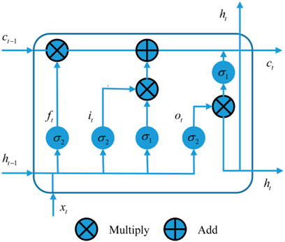
Figure 1 shows the architecture of the established LSTM structure. The LSTM is an enhanced type of RNN, which uses input, output, and forget gates for control. Its key function is to selectively add or delete input information, and the gates provide the path for information to pass. The three gates enhance the memory ability of the network and solve the problem of the disappearing gradient (Lu et al., 2018), (Ramakrishnan and Soni, 2018). The variables are updated in the LSTM as indicated in (Eq. 1):
where the activation function
Attention Mechanism
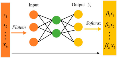
The attention mechanism attempts to mimic the attention of a human. Typically, the human brain focuses on a particular part of an object at a specific moment and gives less attention to the other parts of the object. During the extraction of the sequence features of power grid operational data, the predicted output of the LSTM is affected by noncritical features. The function described by the attention mechanism aids in focusing on the key features of the sequence. The integrated function can be viewed as a key feature extractor, which primarily assigns weights to different features depending on their importance. Figure 2 illustrates the structure of the attention mechanism adopted in this study.
As indicated in the figure, the variable
where
In this study, the attention mechanism is designed to be used after the first layer of the LSTM because the historical operational data has higher dimension than the corresponding transient stability margin data. Therefore, the output features of the first LSTM can be selected through the probability distribution of the attention mechanism with different weights that ensure accurate model prediction.
Prediction Model Based on LSTM Network and AM
Structure of the Proposed Model
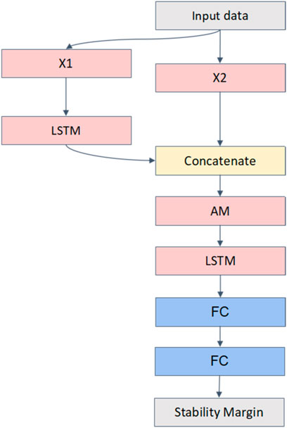
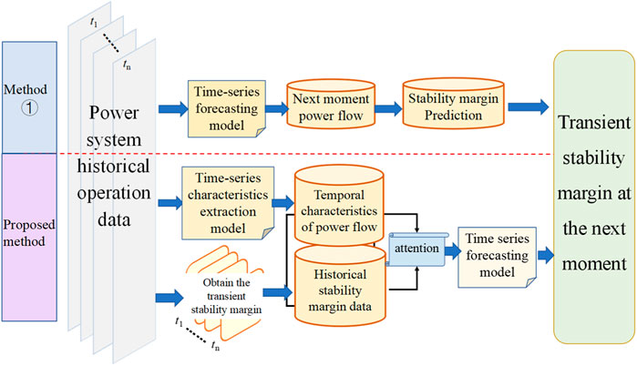
Based on the historical operation data of power grid, on the one hand, temporal characteristics are extracted through a certain model, so that the characterisation of historical power flow operation can be obtained. At this time, the features of the model output are the dimensionality reduction expression of the original input features, which prevents the AM layer from receiving complicated high-dimensional information. Furthermore, the transient stability margin of the power grid in the historical-operation mode is also obtained. Subsequently, the stability margin and the power flow characteristics after the dimensionality reduction are organically integrated through the AM layer, and the multiple weights of the importance of different dimension characteristics are automatically learned. Finally, based on multiple fused features as the input of the time-series prediction model, the transient stability margin of the power grid can be predicted for a future period. Therefore, we developed the model with two LSTM layers, one AM layer, and two fully connected (FC) layers. Figure 3 shows the structure of the proposed model.
In the figure, LSTM indicates the LSTM network layer, AM represents the attention mechanism layer, and FC denotes the FC layer. Additionally, concatenate represents the splicing of the matrix, and the final layer, which is also a regression layer, uses a linear function as the activation function. The remaining layers use the rectified linear unit (ReLU) as the activation function.
Network Input and Output Variables
As shown in Figure 3, the input data are measured from the power grid. The dataset includes the power flow in various branches and the calculated metrics of the transient stability margin. The input data comprise two segments: X1, which is sampled from the active power and reactive power of the branch from t1 to t2, and X2, which is sampled from the values of the transient stability metrics from t1 to t2. Furthermore, the output of the first LSTM layer is concatenated with X2 to serve as the input for the AM layer.
The output of the proposed model is the predicted stability-margin metrics of the continuous t sampling points after t2. The stability-margin metrics are calculated using the trajectory analysis method (Mu et al., 1993). The stability metrics of generator i can be defined using the trajectory-analysis method, as follows:
where
and
Based on the analysis of trajectory
Model Error Analysis and Comparison
The predicted results were evaluated using the root mean square error (RMSE) and mean absolute error (MAE), which are expressed as
where N denotes the total number of samples, and pi and ri indicate the predicted and actual values of the stability metrics of sample i, respectively.
Model Prediction Process
The proposed method predicts the stability margin in two steps: offline training and online prediction.
Offline Training
Different operational modes and fault conditions were set up for the test system through a time-domain simulation to obtain the results under different designed scenarios. The training sample set was established based on the input and output features defined in Network Input and Output Variables. For a sample set with the number of samples N, the feature vectors
The objective of the offline training for the prediction model is to minimise the loss. The most commonly used loss function for a prediction regression is the square loss function. However, this function generates a large penalty for outliers; hence, it is not sufficiently robust. Although the absolute value loss is better than the outlier loss, optimal values cannot be obtained easily owing to its discontinuous derivation. Therefore, Huber loss is used as the loss function in this study, which integrates the square and absolute loss functions [x]. The loss can be calculated using (Eq. 6) as follows:
where ya denotes the actual output value, g(x) indicates the predicted value, and ma represents the threshold value. If the absolute value of the predicted error is lesser or greater than ma, Huber loss represents the square loss or absolute loss, respectively. Therefore, it has the advantages of both the square and absolute losses.
Online Prediction
Online prediction of the stability margin is performed using the input features of the model that are formulated based on the historical data measured from the power grid. When they are input into the trained prediction model, the model can predict the stability-margin metrics of the power grid for a future period.
Case Studies
Data Set Construction
Figure 4 shows the IEEE 39-bus system used for the case study. It comprises 10 generators, 39 buses, 46 branches (including 12 transformer branches), and 19 loads. The reference power and rated frequency of the system are 100 MVA and 60 Hz, respectively.
The 19 loads of the IEEE 39-bus system indicate the actual load values measured from a provincial power grid over a 90-day period. In this period, each load increment was apportioned by all the generators, the measuring interval was 5 min, and a total of 25,920 samples were collected. A three-phase fault occurred at Bus four at the beginning of each measured time with a duration of 0.15 s. Based on the disturbed trajectories of the operating variables of each generator, the stability metrics of each generator corresponding to the fault were calculated. To robustly evaluate the performance of the model (Aly, 2020; Bokde et al., 2020), we used 5-fold cross validation method. And all samples were randomly divided into five groups (each group accounts for 20% of the total samples), one group of data was taken as the testing set, the remaining groups (80% of the total samples) were taken as the training set, and we used the average value of five experiments to compare the performance of the model.
Analysis of Model Prediction Results
We used the Adam network optimizer with 100 iterations, 0.001 learning rate, 128 batch size and set the predicted time step to one during model testing. Table 1 summarises the results in terms of the RMSE and MAE of the predicted transient stability metrics for all generators at input time steps of 5, 10, 15, and 20.
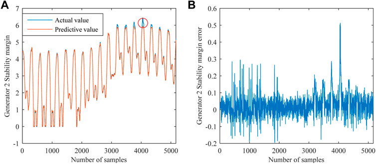
The results in Table 1 indicate that the model exhibits a relatively small error at the four different time steps. We observed that both the error metrics in the case of time step 15 are smaller than those for the other time steps. For one of the 5-fold cross validation experiments, Figure 5 illustrates the actual and predicted stability-margin curves considering generator 2 (Bus 31) as an example; the curves of the absolute error are plotted in Figure 5B. Figure 5 illustrates that the predicted stability margin is close to the actual value based on the model trained using the sample data. The red circle in Figure 5A shows the maximum value of the absolute error occurring on the curve, which is 0.5127. The corresponding relative error is 8.0%, thus indicating adequate prediction characteristics.
Comparison of Performance Based on Different Prediction Methods
To verify the effectiveness of the proposed method, we compared its performance with another method. The input time step was set to 15 and the output was set to 1. As shown in Figure 6, because the historical operation data of the power grid has the temporal characteristics, Method one is to directly input the historical operational data into the corresponding prediction model, so as to obtain the power flow information of the power grid at the next moment, and at the same time, calculate the transient stability margin at the next moment based on the specific information of the power flow and the traditional stability-margin prediction methods. The performances of different prediction methods are shown in Table 2.
The results in Table 2 indicate that the RMSE and MAE obtained using the proposed method are respectively 74.9 and 79.4% less than those obtained using Method 1, and the prediction error is significantly reduced. This is because in the process of constructing the mapping for the machine learning terminal of Method 1, the time-series prediction model is required to directly output the power flow information at the next moment, and the dimension of the output variables is considerably high; moreover, the designed model is highly complex. Therefore, the proposed method performs better than Method one by extracting the temporal characteristics of the operational data to predict the stability margin of the power grid for a future period.
Comparison of Performance Based on Different Input Features
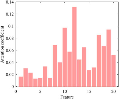
The model input is designed using two segments, namely the branch power flow X1 and transient stability-margin metrics X2. Table 3 summarises the single and double input feature methods with different prediction performances using the same model structure and parameters. The concatenate layer for the splicing matrix is used only in the simulation of double input. Again, the input time step was set to 15 and the output was set to 1. Figure 7 shows the attention coefficients assigned to different features using the attention mechanism layer.
As indicated in Table 3, the RMSE of the double input is 0.0466 and 0.0635 lower than those of the single inputs X1 and X2, respectively. Additionally, the MAE is 0.0345 and 0.0255 lower than the single inputs, respectively. This enhanced prediction validates that the proposed double input feature method exhibits a higher prediction accuracy than the single input feature method with historical power flow or stability margin data.
The horizontal axis in Figure 7 represents different features; numbers 1 to 10 denote the eigenvalues of the branch active and reactive powers after the dimensionality reduction in the first LSTM layer, whereas numbers 11 to 20 indicate the features of the stability-margin metrics of 10 generators. Generally, different features affect the stability-margin prediction in a power grid differently. Considering the ability of the attention mechanism to identify information, the greater the attention coefficient assigned to the feature, the higher is the impact on the prediction. Furthermore, Figure 7 indicates that the attention coefficients from 1 to 10 are not significantly different than those from 11 to 20; the sums of the former and latter are 0.3470 and 0.6530, respectively. Additionally, features X1 and X2, and the stability margin exhibit a strong correlation, verifying that the prediction model should use double input features to train the network. In the following comparative analysis, we also used the double input feature method.
Prediction Performance Analysis Under Changing Topologies
The branch power flow comprises the topology information of the power. To verify the prediction performance of the proposed model under varying topologies, three different proportion samples of topology change were selected to perform the simulation. Each sample randomly switched off one transmission line. Furthermore, the input time step was set to 15 and the output was set to 1. The test results are summarised in Table 4.
As indicated in the table, the difference in the RMSE and MAE values between 30 and 0% topological change are 0.0931 and 0.0510, respectively; the difference in the RMSE and MAE values between 15 and 0% topological change are 0.0645 and 0.0363, respectively. The results indicate that the proposed model exhibits adequate prediction performance under a varying topology.
Comparison and Analysis of Prediction Performance of Different Algorithms
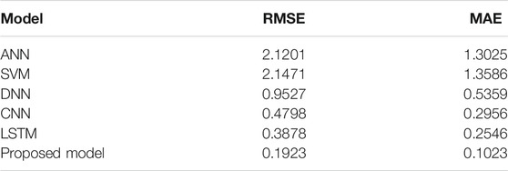
To verify the effectiveness of the proposed model, we compared the simulations with those performed using other common methods, such as artificial neural network (ANN), SVM, deep neural network (DNN), CNN, and LSTM. They concatenate X1 and X2 as inputs to the model. In the ANN and SVM methods, the principal component analysis is used to reduce the dimension of input features, and the optimal model is developed by combining principal component features with the contribution rates over 95%. The ANN is set as a backpropagation neural network with a single hidden layer, and the number of hidden-layer units ranges from 100 to 300. The SVM uses the radial basis function kernel, and the optimal hyperparameters are determined using grid search. For deep learning, the DNN is a modification of the ANN with a deep network, with three, four, or five hidden layers and a corresponding unit number of hidden layers of 100, 200, or 300, which are determined via cross-parameter traversal. The CNN structure comprises two convolution, pooling, and FC layers each. The LSTM structure is configured using two LSTM layers and two FC layers. Furthermore, the activation function and learning algorithm of the ANN, DNN, CNN, and LSTM are consistent with those of the proposed model. And the input time step was set to 15 and the output was set to 1. Table 5 summarises the prediction errors of each model.
The results in Table 5 indicate that the RMSE and MAE values of the proposed model are the smallest in comparison with those of the other models. We observed that the two errors of the LSTM are smaller than those of the other models, except for the proposed model, which verifies the adequate prediction characteristics of the LSTM. The attention mechanism used with the LSTM in the proposed model improved the predictive network, resulting in the enhanced prediction performance.
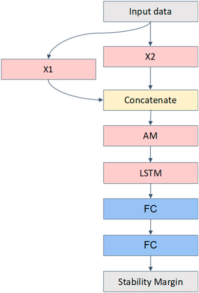
To verify the effectiveness of the two-stage input mode of the proposed model, another model structure (Model 1) was designed based on the LSTM and attention mechanism, and the specific model structure is shown in Figure 8. The original data of the power flow was directly used as input data. The performances of different models are shown in Table 6. The two-stage model proposed in this study also achieves a significant prediction accuracy, which also verifies the effectiveness of reducing the dimension of the historical data X1 using the first layer LSTM network.
Multistep Analysis of Model Prediction
Typically, the output timespan is a critical characteristic of a prediction model, which is essential in industrial applications. Herein, we explore the effect of the output timespan on the proposed model. The input time step was retained as 15, and the output timespan was varied from 1 to 10 for testing. Figure 9 illustrates the characteristic metrics in terms of RMSE and MAE, respectively.

FIGURE 9. (A) RMSE values for different prediction step sizes; (B) MAE values for different prediction step sizes.
As indicated in the figure, the RMSE and MAE values vary with an increment in the output timespan. When the prediction step size is smaller than or equal to six, the RMSE and MAE values obtained using the proposed model are relatively stable, and the maximum differences in comparison with the prediction step size of one are 0.0301 and 0.0231, respectively. When the prediction step size is greater than six, the prediction error of the proposed model increases slightly within a small range. The maximum differences in comparison with the step size of one were only 0.0537 and 0.0619 for the RMSE and MAE, respectively. Therefore, the proposed model ensures high accuracy and stability for the long timespan prediction.
Conclusion
Conventional data-driven transient stability prediction under the concept of security region of power systems can evaluate the stability of only the existing power grid and it does not satisfy the requirements of future predictions. Therefore, an effective prediction method based on the LSTM network and attention mechanism is proposed for the evaluation and prediction of the transient stability margin. The proposed method can effectively determine the stability of a power grid for a future period. The simulation results verify that the proposed model outperforms the conventional machine learning methods. Additionally, the proposed model can abstract the critical features based on the historical power flow and stability metrics dataset; this double input feature and two-stage input mode improve the prediction accuracy. The output timespan value can be selected by the operator to determine the stability trend in advance. The proposed method for the prediction of transient stability margin can be applied to several engineering applications, such as consolidation of the protection and control system, and to avoid severe blackouts.
In the future, we intend to analyse the generalisation performance of the proposed model considering varying system operational modes, network parameters, and topological structures.
Data Availability Statement
The raw data supporting the conclusion of this article will be made available by the authors, without undue reservation.
Author Contributions
JA: Conceptualisation, Methodology, Writing—Original draft preparation. LZ: Writing, Methodology—Original draft preparation. JY: Translation and Validation.
Funding
This work was supported by the National Natural Science Foundation of China (No. 51877034).
Conflict of Interest
The authors declare that the research was conducted in the absence of any commercial or financial relationships that could be construed as a potential conflict of interest.
Publisher’s Note
All claims expressed in this article are solely those of the authors and do not necessarily represent those of their affiliated organizations, or those of the publisher, the editors and the reviewers. Any product that may be evaluated in this article, or claim that may be made by its manufacturer, is not guaranteed or endorsed by the publisher.
Abbreviations
AM, attention mechanism; ANN, artificial neural network; CNN, convolutional neural network; DNN, deep neural network; FC, fully connected; LSTM, long short-term memory; MAE, mean absolute error; ReLU, rectified linear unit; RMSE, root mean square error; RNN, recurrent neural network; SVMs, support vector machines.
References
Aly, H. H. (2020). A Novel Deep Learning Intelligent Clustered Hybrid Models for Wind Speed and Power Forecasting. Energy 213, 118733. doi:10.1016/j.energy.2020.118773
An, J., Al, S., Liu, D., Li, B., Shao, G., Xu, X., et al. (2019). A Power System Transient Stability Assessment Method Based on Short-Time Disturbed Trajectories. Power Syst. Technol. 43 (5), 1690–1696. doi:10.13335/j.1000-3673.pst.2018.1947
An, J., Yu, J., Li, Z., Zhou, Y., and Mu, G. (2020). A Data-Driven Method for Transient Stability Margin Prediction Based on Security Region. J. Mod. Power Syst. Clean Energ. 8 (6), 1060–1069. doi:10.35833/mpce.2020.000457
Bera, A., Wharton, Z., Liu, Y., Bessis, N., and Behera, A. (2021). Attend and Guide (AG-Net): A Keypoints-Driven Attention-Based Deep Network for Image Recognition. IEEE Trans. Image Process. 30, 3691–3704. Mar. 2021. doi:10.1109/TIP.2021.3064256
Bokde, N. D., Yaseen, Z. M., and Andersen, G. B. (2020). ForecastTB—An R Package as a Test-Bench for Time Series Forecasting—Application of Wind Speed and Solar Radiation Modeling. Energies 13 (10), 2578. doi:10.3390/en13102578
Cheng, J., Dong, L., and Lapata, M. (2016). “Long Short-Term Memory Networks for Machine Reading,” in Proceedings of the 2016 Conference on Empirical Methods in Natural Language Processing, Austin, TX (New York, NY: Association for Computational Linguistics), 551–561. doi:10.18653/v1/d16-1053
Dengkai, M., Tong, W., Yuwei, X., and Wenjuan, D. (2020). Elastic Net Based Online Assessment of Power System Transient Stability Margin. Power Syst. Technol. 44 (1), 19–26. doi:10.13335/j.1000-3673.pst.2019.0687
Du, Y., Hu, Z., Li, B., Chen, J., Weng, C., et al. (2021). Transient Stability Assessment of Power System Based on Bi-directional Gated Recurrent Unit. Automation Electric Power Syst. 45 (20), 103–112. doi:10.7500/AEPS20210118001
Gao, K. L., Yang, S., Liu, S., and Li, X. (2019). Transient Stability Assessment for Power System Based on One-Dimensional Convolutional Neural Network. Automation Electric Power Syst. 43 (12), 18–26. doi:10.7500/AEPS20180911006
Huankun, Z., Xianrong, C., and Zhenghui, W. (2012). Application of High Precision and A-Stability Implicit Tuned Taylor Series Method in Power System. Trans. China Electrotechnical Soc. 27 (1), 217–223. doi:10.19595/j.cnki.1000-6753.tces.2012.01.031
Karami, A. (2011). Power System Transient Stability Margin Estimation Using Neural Networks. Int. J. Electr. Power Energ. Syst. 33 (4), 983–991. doi:10.1016/j.ijepes.2011.01.012
Kardakis, S., Perikos, I., Grivokostopoulou, F., and Hatzilygeroudis, I. (2021). Examining Attention Mechanisms in Deep Learning Models for Sentiment Analysis. Appl. Sci. 11 (9), 3883. doi:10.3390/app11093883
Li, B., Wu, J., Hao, L., Shao, M., Zhang, R., and Zhao, W. (2020). Anti-Jitter and Refined Power System Transient Stability Assessment Based on Long-Short Term Memory Network. IEEE Access 8, 35231–35244. doi:10.1109/access.2020.2974915
Lu, Z., Lv, W., Zhipu, X., and Zhu, T. (2018). “Highway Traffic Volume Prediction via Stacking KNN, SVR, MLP, RNN,” in IEEE SmartWorld, Ubiquitous Intelligence & Computing, Advanced & Trusted Computing, Scalable Computing & Communications, Cloud & Big Data Computing, Internet of People and Smart City Innovation (SmartWorld/SCALCOM/UIC/ATC/CBDCom/IOP/SCI), Guangzhou, China, 1408–1413.
Luong, M. T., Pham, H., and Manning, C. D. (2015). “Effective Approaches to Attention-Based Neural Machine Translation,” in Proceedings of the 2015 Conference on Empirical Methods in Natural Language Processing, Stroudsburg, PA (Lisbon, Portugal: Association for Computational Linguistics), 1412–1421. doi:10.18653/v1/d15-1166
Mu, G., Wang, Z., Han, Y., and Huang, M. (1993). A New Method for Quantitative Assessment of the Transient Stability of Power Systems-Trajectory Analysis Method. Proc. CSEE 13 (3), 25–32. doi:10.13334/j.0258-8013.pcsee.1993.03.004
Ramakrishnan, N., and Soni, T. (2018). “Network Traffic Prediction Using Recurrent Neural Networks,” in 17th IEEE International Conference on Machine Learning and Applications, Orlando, USA, 17-20 Dec. 2018, 187–193. doi:10.1109/icmla.2018.00035
Shi, Z., Yao, W., Zeng, L., Wen, J., Fang, J., Ai, X., et al. (2020). Convolutional Neural Network-Based Power System Transient Stability Assessment and Instability Mode Prediction. Appl. Energ. 263, 114586. doi:10.1016/j.apenergy.2020.114586
Su, F., Yang, S., Wang, H., and Zhang, B. (2017). Study on Fast Termination Algorithm of Time-Domain Simulation for Power System Transient Stability. Proc. CSEE 37 (15), 4372–4378. doi:10.13334/j.0258-8013.pcsee.161491
Wang, B., Fang, B., Wang, Y., Liu, H., and Liu, Y. (2016). Power System Transient Stability Assessment Based on Big Data and the Core Vector Machine. IEEE Trans. Smart Grid 7 (4), 2561–2570. doi:10.1109/tsg.2016.2549063
Wang, Z., Zhou, Y., Guo, Q., and Sun, H. (2021). Transient Stability Assessment of Power System Considering Topological Change:a Message Passing Neural Network-Based Approach. Proc. CSEE 41 (7), 2341–2350. doi:10.13334/j.0258-8013.pcsee.202139
Wu, W., Tang, Y., Sun, H., and Xu, S. (2012). A Survey on Research of Power System Transient Stability Based on Wide-Area Measurement Information. Power Syst. Technol. 36 (9), 81–87. doi:10.13335/j.1000-3673.pst.2012.09.016
Yan, R., Geng, G., Jiang, Q., and Li, Y. (2019). Fast Transient Stability Batch Assessment Using Cascaded Convolutional Neural Networks. IEEE Trans. Power Syst. 34 (4), 2802–2813. doi:10.1109/tpwrs.2019.2895592
Yuanhang, D., Lei, C., Weiling, Z., Yong, M., and Wenfeng, L. (2016). Power System Transient Stability Assessment Based on Multi-Support Vector Machines. Proc. CSEE 36 (5), 1173–1180. doi:10.13334/j.0258-8013.pcsee.2016.05.001
Zhang, X., Wang, Y., Zheng, Y., Ding, R., Chen, Y., Wang, Y., et al. (2020). Reactive Load Prediction Based on a Long Short-Term Memory Neural Network. IEEE Access 8, 90969–90977. doi:10.1109/access.2020.2991739
Keywords: attention mechanism, long short-term memory, temporal characteristics, transient stability, stability margin
Citation: An J, Zhang L, Zhou Y and Yu J (2022) Transient Stability Margin Prediction Under the Concept of Security Region of Power Systems Based on the Long Short-Term Memory Network and Attention Mechanism. Front. Energy Res. 10:838791. doi: 10.3389/fenrg.2022.838791
Received: 18 December 2021; Accepted: 07 March 2022;
Published: 29 March 2022.
Edited by:
Ke Meng, University of New South Wales, AustraliaReviewed by:
Neeraj Dhanraj Bokde, Aarhus University, DenmarkZehua Zhao, The University of Sydney, Australia
Copyright © 2022 An, Zhang, Zhou and Yu. This is an open-access article distributed under the terms of the Creative Commons Attribution License (CC BY). The use, distribution or reproduction in other forums is permitted, provided the original author(s) and the copyright owner(s) are credited and that the original publication in this journal is cited, in accordance with accepted academic practice. No use, distribution or reproduction is permitted which does not comply with these terms.
*Correspondence: Yibo Zhou, emhvdXlpYm9hYUAxMjYuY29t
 Jun An
 Yibo Zhou