Loss Prediction of Ultrahigh Voltage Transmission Lines Based on EEMD–LSTM–SVR Algorithm

Line loss prediction of ultrahigh voltage transmission lines is the key for ensuring the safe, reliable, and economical operation of the power system. However, the strong volatility of line loss brings challenges to the prediction of transmission line loss. For more accurate prediction, this article uses ensemble empirical mode decomposition (EEMD) to decompose the line loss and proposes the EEMD–LSTM–SVR prediction model. First of all, this article performs feature engineering on power flow, electric energy, and meteorological data and extracts the exponentially weighted moving average (EWMA) feature from the line loss. After the integration of the time dimension, this article mines the curve characteristics from the time series and constructs a multidimensional input dataset. Then, through ensemble empirical mode decomposition, the line loss is decomposed into high-frequency, low-frequency, and random IMFs. These IMFs and the standardized multidimensional dataset together constitute the final input dataset. In this article, each IMF fusion dataset is sent to LSTM and support vector regression models for training. In the training process, the incremental cross-validation method is used for model evaluation, and the grid search method is used for hyperparameter optimization. After evaluation, the LSTM algorithm predicts high-frequency IMF1 and 2 and random IMF4 and 5; the SVR algorithm predicts low-frequency IMF6 and 7 and random IMF3. Finally, the output value of each model is superimposed to obtain the final line loss prediction value. Also, the comparative predictions were performed using EEMD–LSTM, EEMD–SVR, LSTM, and SVR. Compared with the independent prediction models EEMD–LSTM and EEMD–SVR, the combined EEMD–LSTM–SVR algorithm has a decrease in mean absolute performance error% by 2.2 and 25.37, respectively, which fully demonstrates that the combined model has better prediction effect than the individual models. Compared with that of SVR, the MAPE% of EEMD–SVR decreases by 11.16. Compared with that of LSTM, the MAPE% of EEMD–LSTM is reduced by 32.72. The results show that EEMD decomposition of line loss series can effectively improve the prediction accuracy and reduce the strong volatility of line loss. Compared with that of the other four algorithms, EEMD–LSTM–SVR has the highest R-square of 0.9878. Therefore, the algorithm proposed in this article has the best effectiveness, accuracy, and robustness.

1 Introduction

Line loss is an essential indicator of economic operation in the power system, which affects the planning and design, production, and management of power enterprises (Wang et al., 2020). The difference between the actual power supply and power sales obtained by statistics is the actual line loss of the grid, called statistical line loss. Statistical line losses are generated by running lines, natural disasters, artificial power theft, and inaccurate statistical measurement. No matter what the cause of line loss is, it will have an immeasurable impact on the economic profit of power supply enterprises. Therefore, it is necessary to formulate targeted energy-saving and loss reduction measures, study accurate line loss prediction methods, and build a comprehensive calculation system to improve the economic operation of power grids and enhance the line loss management capability of power supply enterprises.

China’s primary energy sources are mainly distributed in the west, while the economic development centers are primarily in the center and east. This inverse distribution pattern determines the transmission pattern of China from west to east. Therefore, China’s UHV transmission technology has developed rapidly, and a lot of UHV transmission lines have been built and put into operation (Huang et al., 2009). UHV transmission plays a vital role in power transmission, and how to build UHV power grids economically and efficiently is an important issue that needs to be carefully studied. Transmission losses are an essential factor affecting UHV transmission projects’ economics. Transmission losses include substation losses and transmission line losses; substation losses include station equipment losses and station consumption, which change proportionally with the change of transmission load. Also, transmission line loss mainly includes resistance and corona loss. Corona loss is closely related to line voltage, conductor structure, and climatic conditions (Liang et al., 2020).

There are few studies on the statistical line loss of UHV transmission lines. The traditional methods use overly simplified calculation models and processing methods to simplify the calculation process, which cannot meet the requirements of today’s power supply enterprises for line loss management. Among the many causes of line loss anomalies in the UHV transmission system, power theft is always one of the most dominant causes of line loss anomalies. In addition to electricity theft, common causes of line loss anomalies in the actual grid include meter breakdown, unmetered use, unattended use, and collection errors. Electricity theft refers to the user through technical means to achieve for the meter measurement becomes less or not measured and then achieve the purpose of illegal use of electricity. Existing traditional power-theft detection methods mainly have the following problems: 1) manual screening of user power-theft is difficult; 2) detection process is too complex; 3) low screening efficiency; and 4) the required labor costs are huge (Jindal et al., 2016).

In general, offline calculation and online measurement require a lot of time, material, and financial resources, while the forecast can predict the amount of line loss, and then take appropriate measures. It can be said as the relative reduction of the operator’s maintenance pressure and financial pressure. Electricity supply companies lack a fast and effective method for identifying line losses caused by electricity theft. Therefore, researching a fast and accurate line loss prediction technology is essential to improve the security and stability of the power grid.

In recent years, with the vigorous development of large-scale data, artificial intelligence, and other advanced technologies, the traditional power grid has transformed into a smart grid, and smart meters and power user electricity collection systems have gradually become popular in power supply enterprises. After long-term data accumulation, China’s power enterprises have accumulated a large amount of historical electricity consumption information, and there are three main types of data: the first is power production data, including line loss and power data; the second is power consumption data stored in the marketing process of power enterprises, including power sales and customer information; and the third is power enterprise management data, including equipment maintenance and other data. These data are an important basis for line loss analysis and line loss management, but at present, power supply enterprises do not have a high utilization in the face of massive data and cannot realize effective, fast, and efficient analysis, thus failing in line loss abnormality analysis. In recent years, power supply enterprises are trying to use new Internet technologies such as rapidly developing automation technology, information and communication technology, data mining, and deep learning to integrate existing isolated and scattered power information and establish a UHV network line loss monitoring and analysis system with reliable and smooth operation, high information sharing, and effective data integration, so as to effectively reduce losses and save energy and realize economic operation of the power grid.

For specific measures to reduce losses, a demand analysis can be conducted for power suppliers. Then, a suitable development platform is selected to determine and diagnose the causes of abnormal line loss areas, while logic analysis and development design are carried out to launch the line loss abnormal intelligent diagnosis system. The system mainly includes software function modules such as storage and management, line loss abnormality area query, line loss abnormality diagnosis and analysis, missing data filling, and closed-loop management. It realizes effective analysis and scientific diagnosis of line loss abnormalities, fine management of line loss, and improves the efficiency of line loss management. As the main input data of the intelligent diagnosis system for line loss abnormalities, only improving the prediction accuracy can ensure the reliability, effectiveness, and accuracy of the intelligent diagnosis system (Yan et al., 2016).

Suppose artificial intelligence algorithms are used to predict line loss, in that case, the powerful self-learning, generalization, and nonlinear processing capabilities of neural networks can be used to fit the relationship between the line loss and the characteristic parameters. The accuracy of the prediction method and the richness of the output results are in line with the rapid development of the power industry. For the grassroots managers of power grids, line loss has a direct guiding role in daily line maintenance and management (Song, 2019). Accurate line loss forecasting helps managers to understand line loss trends, promptly respond to line loss anomalies, and quickly investigate and adjust line operation patterns. There are a few cases in which the statistical line loss does not match the actual value due to various influences such as abnormal equipment collection, load transfer, and switching of power supply for dual power users. The comparison between the predicted and actual values of line loss can assist in verifying the accuracy and reliability of UHV-network’s data measurement and network topology connection. In addition, other traditional detection methods include hardware status-based detection methods, which use special equipment to improve detection accuracy, but are costly to implement and require unannounced manual inspection and random testing of on-site power equipment, which is ineffective and time-consuming. The conventional manual screening-based line loss management method does not effectively reflect the interrelationship between power data, which limits the real-time and accuracy of line loss analysis and line loss abnormality diagnosis, and seriously limits the efficiency of line loss management, especially with the popularization and application of smart meters, the traditional manual conduct of regional periodic spot checks and other inefficient power theft inspection methods are gradually being eliminated.

Each individual AI algorithm has advantages and disadvantages, for example, the SVR algorithm is fast to train, and the LSTM has a strong predictive power for sequences with strong jitter. To improve the prediction accuracy and reduce the training time, a combined model can be used for line loss prediction. To this end, the EEMD–LSTM–SVR algorithm is proposed in this article, using EEMD for modal decomposition and the combined LSTM–SVR model for prediction and using incremental cross-validation and grid search tuning methods to verify model validity and robustness. The objectives of this study are as follows:

• Existing studies on line losses mainly focus on medium and low voltage transmission networks, and there are few studies on ultra-high voltage transmission line losses. In this article, after carefully investigating the causes of line loss in EHV transmission lines, we establish a multidimensional model input system to extend the line loss prediction to the high voltage domain.

• To address the difficulty of existing models to handle strong jitter signals, this article first uses EEMD to perform decomposition of line loss sequences.

• To improve the model prediction accuracy and model training speed, this article uses SVR to predict the IMF with stronger regularity to improve the training speed and LSTM to predict the IMF with strong jitteriness to improve the accuracy.

The research object of this article is the line loss prediction of ultrahigh voltage transmission lines. First, use EEMD to decompose the line loss data. Then, combine the decomposed IMFS with active power, reactive power, line current and voltage, and regional meteorological data. The final dataset is fed into an LSTM or SVR model for model training, and incremental cross-validation and grid search are used to enhance model performance and complete model evaluation, followed by line loss forecasting for the next 3 months. Experiments have proved that the EEMD–LSTM–SVR model proposed in this article has a better prediction effect than other models.

This article proposes a UHV line loss forecasting method based on EEMD and LSTM–SVR. The novelty of this study is as follows: 1) use LSTM to predict complex high-frequency IMFs, and use SVR to predict regular low-frequency IMFs to make the results more accurate; 2) the combination of EEMD and LSTM–SVR makes the model more sensitive to changes in the tag value and ultimately manifests itself as an improvement in prediction accuracy; 3) the vision of line loss prediction is extended to the UHV field, not limited to the distribution network; 4) incremental cross-validation is used to validate the model training process, interspersed with grid searches to tune the model parameters. Based on multiple iterations of the prediction process, incremental cross-validation ensures the realism and robustness of the prediction model.

The rest of this study is structured as follows: Section 2 provides a literature review. Section 3 provides feature engineering. Section 4 describes the modeling process of EEMD–LSTM–SVR. Section 5 provides a case study. Section 6 presents concluding remarks.

In conclusion, with the rapid development of UHV transmission technology in China, how to build UHV power grid economically and effectively has become a top priority, and transmission losses have an important impact on the economics of UHV power grid. At the same time, the current research on line loss mainly revolves around medium and low voltage distribution networks, and there is little research on UHV line loss. Therefore, this article focuses on the prediction of line losses in the UHV transmission process and proposes a combined prediction model EEMD–LSTM–SVR, which combines the modal decomposition method with the combined model to effectively cope with the challenges brought by the strong jitter of line loss sequences. First, the decomposition helps the model to filter out the complex noise in the line loss sequence and fully exploit the line loss pattern. Second, compared with independent prediction models, choosing the appropriate prediction model for each IMF will greatly improve the prediction accuracy. Third, the selection of SVR for prediction of IMFs with stronger regularity helps to improve the model training speed. To demonstrate the effectiveness of the combined prediction models, extensive literature will be cited in the following to illustrate.

2 Literature Review

To improve the accuracy of line loss prediction, existing studies mainly focus on mining the complex mapping relationships between various influencing factors and line loss through prediction models (Peng et al., 2021). The whole prediction process can be divided into data preprocessing, model construction, and evaluation. The most crucial part of data preprocessing is the feature selection in dataset construction, which will directly affect the training effect of the model (Sahlin et al., 2017). UHV transmission line losses are heavily influenced by meteorology, and line losses on rainy and snowy days increase exponentially compared to those on nice days. Existing models are poor learners of meteorological factors, but if the long-term relationships of hourly time series data from power markets, local weather, and calendars are considered, the model prediction accuracy will substantially improve (Tulensalo et al., 2020). In Zhong et al. (2020), 32,000 stations in a city are taken as the research object, which pays not only attention to its line parameters and power but also attention to the number of users and residents in the station and the total number of electric energy meters in the station, which can further explore the main factors affecting the line loss rate in the station. The research in this article is about high voltage transmission line losses, which are more sharply influenced by weather, so meteorological factors, power system tide data, and electrical energy data are considered.

In the model construction, using accurate predictive models allows for better reliable and accurate planning and scheduling of the UHV transmission system to ensure the benefits of grid companies. However, line losses’ highly chaotic, intermittent, and stochastic behavior implies a high degree of difficulty in predicting line losses. Therefore, the use of ensemble empirical mode decomposition (EEMD) for line loss prediction, which decomposes original highly irregular values into regular IMFs, helps to reduce the difficulty of line loss prediction and plays a vital role in guiding the operational planning of the UHV transmission system. The EEMD is an empirical decomposition method that decomposes a time series into numerous subseries according to different frequencies. EEMD is used as a preprocessing technique for hybrid forecasting models. Different prediction models are used to predict the subsequences generated by the decomposition. In this article, line loss generation is somewhat random, and it is challenging to find periodic patterns. EEMD decomposes line losses into IMFs with regularity, and the model will learn the line loss patterns more accurately and perform better in line loss predictions (Bokde et al., 2019). Common decomposition methods include wavelet, empirical modal decomposition, seasonal adjust methods, variational modal decomposition, and intrinsic time-scale decomposition methods (Bokde et al., 2021).

As for the algorithm selection in model construction, in recent years, based on the large amount of data generated by the operation of the power system and the development of artificial intelligence algorithms, traditional line loss calculation methods have gradually developed to intelligent processing algorithms represented by artificial neural networks (Zhang et al., 2018). The least squares support vector machine (LSSVM) can be used for both classification and prediction (Bokde et al., 2019; Chen et al., 2021; Xia et al., 2021). The support vector regression (SVR) improves the LSSVM, which significantly increases the speed of operation (Liu et al., 2019). In addition, if the model parameters are further optimized, higher prediction accuracy can be achieved (Tan et al., 2015). Some studies perform principal component analysis (PCA) and cluster analysis on the influence factors, or decomposition on the target, to help the model be better trained (Zhou et al., 2018). After these optimizations, the model can perform well even when the target values contain complex noise or substantial jitter (Wu and Peng, 2016).

In addition to LSSVM and SVR algorithms, other machine learning models are also applied for prediction. Chang combined the radial basis function (RBF) neural network and enhanced particle swarm optimization (EPSO) for forecasting (Chang, 2013). In order to reduce huge losses brought by line loss, Tao et al. developed a simultaneous prediction system based on PCA and improved the CHAID decision tree (Tao et al., 2019). Yao et al. established gradient boosting decision tree (GBDT) model for predicting the line loss rate, which can identify the complex and nonlinear relationship between line loss and other factors (Yao et al., 2019). GBDT adopts the boosting idea based on the random forest, which can build a weak learner at each iteration step to make up for the shortcomings of the original model. Random forest and SVM are regarded as the two best traditional machine learning algorithms.

In the field of deep learning, Liu et al. proposed a novel method based on the quantum genetic algorithm (QGA) and BP neural network to accurately predict line loss (Liu et al., 2011). Artificial neural networks (ANNs) can also be used for forecasting (Alamin et al., 2020; Ti et al., 2021). Li et al. described a forecasting method based on recurrent neural network (RNN), which can discover nonlinear features and invariant structures exhibited in date and labels (Li et al., 2019). Xin et al. presented a BP network for line loss prediction, which has a stronger nonlinear mapping ability (Xin et al., 2002). In Tulensalo et al. (2020), A long–short memory (LSTM) recurrent neural network model for line loss prediction is proposed, which learns the laws of electric energy, seasonality, and weather effects. RNN and LSTM have unique advantages in processing time-series. To deal with the complex noise in the target value, noise reduction or modal decomposition is often carried out before sending it into the model. Zhou et al. established a daily line loss rate prediction model of a power distribution network based on the combination of denoising auto-encoder (DAE) and long short-term memory network (LSTM) (Zhou et al., 2021). The experimental results show that the model has high accuracy in predicting the daily line loss rate, moderate calculation speed, and practical value in engineering applications. Deng et al. (2019) considered that the actual line loss is affected by many factors such as measurement, management, and communication. He also proposes a deep neural network (DNN) to analyze the internal relationship between different influencing quantities. This article adds ensemble empirical mode decomposition (EEMD) on this basis of Zhou et al. (2021). Through combined SVR with LSTM, the experiments have proved that the model prediction will have higher accuracy (Miraftabzadeh et al., 2021).

The aforementioned works of literature used neural network or machine learning algorithms to forecast the transmission line loss; most of them are for distribution network line loss calculation. However, there are few kinds of research on the prediction of UHV line loss. UHV line loss and distribution network line loss have both difference and connection. Therefore, these neural network models are significant for calculating UHV line loss.

Each of the aforementioned single models for line loss prediction has advantages and disadvantages, whereas to improve the prediction performance, hybrid models combine different methodologies with taking advantage of each method. Decomposition-based hybrid models that take advantage of time-series decomposition methods have been reported frequently. It is widely accepted that line loss time-series are highly volatile and nonstationary. It is challenging to model the original time-series by a single method. Decomposition-based methods take advantage of decomposition methods, in which the original time series can be decomposed into different subseries, which can be modeled more effectively than the original time series. In this article, a combined model prediction method based on EEMD decomposition is proposed for line loss time-series. The high-frequency IMFs will get better prediction results using the deep learning method (LSTM) due to the high-frequency jitter nature, while the low-frequency IMFs uses the machine learning algorithm (SVR) to improve the model prediction speed, and for the random component, the prediction results of the two models are compared to choose a better one (Zheng et al., 2019; Liu et al., 2021).

In terms of model evaluation, the performance of forecasting methods is related to many factors, and existing studies focus more on the nature of the time series itself and the choice of forecasting models. Each forecasting process should be studied and matched with a full range of aspects such as seasonality and trend of the data and stochastic parameters of the model. Sometime, a model will fit better for datasets with seasonality and perform poorly for data with trend and stochasticity. In addition, the error evaluation function of the model can also have an impact on the prediction results. In this article, we use incremental cross-validation to validate the model training process, interspersed with grid searching to tune the model parameters. The cross-validation process iterates over the model several times to ensure the realism and robustness of the models (Bokde et al., 2020; Sun et al., 2021).

In view of the research gap mentioned previously, this study adopts the combined EEMD–LSTM–SVR prediction model with shorter training time and stronger mapping capability to predict the UHV line loss and uses incremental cross-validation and grid search tuning methods to verify the model validity and robustness. Compared with EEMD–LSTM, EEMD–SVR, LSTM, and SVR algorithms, the proposed method performs best on MAPE%, SMAPE%, MAE, MSE, RMSE, and R².

3 Feature Engineering

The characteristics of electric energy loss in UHV transmission are obviously different from those in the distribution network. In addition to the resistance loss, there is also corona loss in UHV transmission. Resistance loss is caused by resistance heating when the currents flow through the conductor. Corona loss is caused by the corona phenomenon, which is significantly affected by weather conditions and air humidity. This article selects a 1,000-kV transmission line as the research object. After comprehensive consideration from the actual situation to the difficulty of data acquisition, choose the running-state of the line parameters, including active power, reactive power, voltage, and current. Meteorological factors such as humidity, wind speed, temperature, atmospheric pressure, and other factors are selected. The preprocessing for the aforementioned factors is as follows (Baran et al., 2013; Rudolf et al., 2019; Simões et al., 2020; Savian et al., 2021):

3.1 Preprocessing of Time Series Data

Operating data of transmission lines consist of various factors. Data structures are diverse from time scales to formats, and it appears challenging to mine the information and utilize the data adequately. The data such as power flow, electric energy, and weather are called time series data because of their relationship with the recording time. Due to the different settings of measuring instruments, there are differences in time scale and recording frequency among time series data. Therefore, it is necessary to clean and aggregate data to construct a normalized timing dataset. In this article, measured data of the power grid transmission lines are normalized; thus, a structured historical transmission line database is constructed. The technical route is shown in Figure 1. The data used in this article are summarized in Table 1.

FIGURE 1

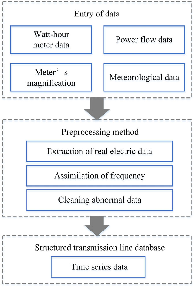
FIGURE 1. Flowchart of data preprocessing.

TABLE 1

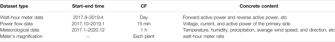
TABLE 1. Table of raw data.

The data measured using a watt-hour meter, monthly power flow data, and meteorological data are in different measuring frequencies. Data measured using a watt-hour meter are recorded daily, power flow data are recorded every 15 min, and meteorological data are recorded every hour. It is necessary to clean power flow data and meteorological data to the maximum time scale to realize accurate aggregation in the time dimension.

According to long-term practical experience and the data collected by the electricity department for many years, it can be seen that lightning, rainstorm, hottest temperatures, and other extreme weather will have a significant impact on power generation, transmission, and electricity consumption (Zainuddin et al., 2020; Audinet et al., 2014).

Under extreme weather, the line loss of transmission lines is prone to abnormal increases, such as increases of resistance loss caused by the hottest temperatures and corona discharge caused by intense convection weather. Therefore, the preprocessing of daily meteorological data is shown in Table 2. After considering severe weather phenomena, the dissimilated data processing method is adopted to deal with different influences of meteorological factors on transmission lines (Li et al., 2011; Khan and Islam, 2019; Huang et al., 2021).

TABLE 2

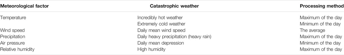
TABLE 2. Dissimilation treatment table of meteorological factors.

As for power flow data, choose the average as an observed value under the diurnal time granularity. After the aforementioned processing, the frequency of data is unified on a day-scale, and the transmission line’s operating dataset is aggregated according to the recording time.

3.2 EWMA Feature Construction of Line Loss

Exponentially weighted moving average (EWMA) is often used to describe trends of time series. It considers the high weight of recent data and at the same time gradually reduces the weight of recent data to compensate overall trend. This method can forecast the future trend of line loss and enrich datasets further (Agami, 2011).

The process of constructing the EWMA feature is as follows: for the daily line loss sequence of one line, n is the number of samples of line loss sequence, and the EWMA feature of daily line loss is calculated by Eq. 1.

$\{\begin{array}{c}{e}_i=l_0,i=\mathrm{0,1}\\ e_i=(1-\alpha )e_{i-1}+\alpha l_{i-1},i=\mathrm{2,3}\dots n\\ e_i=(1-\alpha )e_n+\alpha l_n,i>n\end{array},(1)$

where $\alpha$ is the smoothing parameter. The value range of $\alpha$ is $\left(\mathrm{0,1}\right]$, and the differential evolution method is used to minimize the objective function to obtain the optimal $\alpha$ value. The calculated objective is shown in Eq. 2:

$\alpha =\arg \min \left({\displaystyle \sum _{i=1}^N\sqrt{{\left(l_i-e_i\right)}^2}}\right).(2)$

As shown in Eq. 1, EWMA feature after day $n+1$ will remain unchanged, seriously affecting the accuracy of medium- and long-term line loss calculations. Considering the relation between line loss and time distribution of power supply, line loss data sequences are broken into six parts: Monday, Tuesday, Wednesday, Thursday, Friday, and the weekend. Calculating EWMA characteristics of each class and aggregating six EWMA characteristics in the date order. Figure 2 shows the variation of actual statistical line loss and the EWMA feature of 1,000-kv transmission line.

FIGURE 2

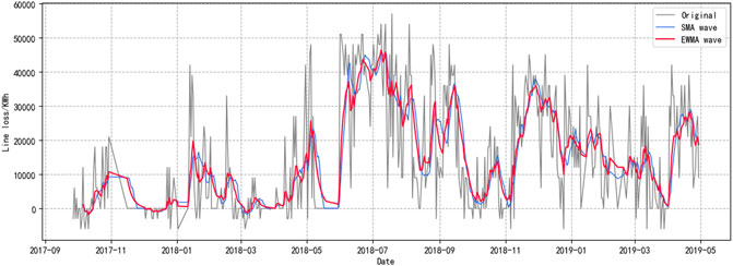
FIGURE 2. EWMA feature of transmission line.

The red line in Figure 2 is EWMA, which can reflect the trend of line loss changing shortly and provide reference information for line loss prediction in the next period. The blue line in Figure 2 is the simple moving average characteristic (SMA). SMA is the average value of line loss of N days before a certain date node, which is a simple extraction of line loss changing trend. The EWMA feature can extract the trend of line loss in the time range while eliminating the influence of complex noise and enriching the dataset.

3.3 Curve Feature Construction of Time Series Data

Curve features include average, minimum, maximum, and average difference values used to describe the average trend and extreme value of time series data and changes of time series data on different days. For time-series data of impact quantity $V$, $V_w^i$ means impact quantity within time-window w, where date $i$ changes from 1 to 7. Equations 3 and 4 show calculation of $V_{mean}$ and $V_{mean\_diff}$. The time-window $w$ is set as 7 days according to experience. Drawing humidity curves of 1,000-kV transmission line as shown in Figure 3.

$V_{mean}={\displaystyle \sum _{i=1}^w{v}_w^i/w},(3)$

$V_{mea{n}_{-}diff}={\displaystyle \sum _{i=2}^w\left(v_w^i-v_w^{i-1}\right)}/(w-1),(4)$

FIGURE 3

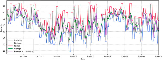
FIGURE 3. Humidity curve characteristic chart.

The construction of curve features of time series data can maximize data features and help in model learning. Utilizing the average value, extremum, and average difference value, the olfactory sense of the line loss calculation model will be more sensitive. Data of only one dimension are expanded to four dimensions. With the increase of data volume, the model can also get better predicting results.

4 Methodology

4.1 EEMD

Line loss sequence is an original nonstationary signal, and empirical mode decomposition (EMD) is a decomposition method used to deal with nonlinear and nonstationary signals. The decomposition results of EMD are shown in Eq. 5 (Zhou et al., 2019).

$X\left(t\right)={\displaystyle \sum _{i=1}^n{C}_i}\left(t\right)+r_n\left(t\right),(5)$

where $c_i\left(t\right)$ is a IMF component, and $r_n\left(t\right)$ is residual.

The EMD processing flow is as follows:

1) The extreme points of the original signal $X\left(t\right)$ are demarcated; all the extreme points are collected to form the upper and lower envelope ($l_1{l}_2$). $m_1$ is obtained through processing for envelope ($l_1{l}_2$).

$m_1=\left(l_1+l_2\right)/2.(6)$

Calculate the residual of the original signal $m_1$ and $h_1$:

$h_1=X\left(t\right)-m_1.(7)$

Iterate until $h_k$ reaches the constraint requirements, denoted as $C_1$ (IMF₁).

2) Calculate the difference between the original signal and IMF1 as a calculation input $r_1$ of the new round:

$r_1=X\left(t\right)-C_1.(8)$

3) Repeat the aforementioned steps, and finally get n IMFs and residual components $r_n\left(t\right)$.

In the process of power operation, there will be intermittent signals in the statistical line loss. The modal aliasing phenomenon occurs in the decomposition process of EMD, resulting in poor expression of IMF components. But, EEMD adds the white noise in the original statistical line loss, which can perfectly deal with the previous problem.

The EEMD processing flow is as follows:

1) Add a group of white noise signals to the original data.

2) Perform EMD decomposition on the new sequence.

3) Repeat the EMD decomposition, adding white noise of different amplitude each time to obtain N groups of IMF components and residual sequences.

4) Perform intermediate processing on the N groups of IMF components, and integrate them to obtain the EEMD decomposition result.

4.2 LSTM

The long short-term memory network (LSTM) solves the gradient disappearance of the recurrent neural network (RNN) during remote transmission. LSTM currently has an excellent performance in natural language processing and time series prediction. The basic unit structure diagram is shown in Figure 4 (Wen et al., 2019).

FIGURE 4

FIGURE 4. Schematic diagram of the basic unit structure of LSTM.

In Figure 4, X_t and h_t are the input and output of the basic unit at time t, i_t and f_t are the output of the input gate and forget gate at time t, respectively, O_t is the output of the outputting-gate at time t, and g_t is the unit state at time t. The specific calculation equations are as follows:

1) Input status.

$g_t=\tanh \left(W_{ig}{x}_t+b_{ig}+W_{hc}{h}_{t-1}+b_{hg}\right),(9)$

2) Gating status.

$i_t=sigmoid\left(W_{ij}{x}_t+b_{ii}+W_{hi}{h}_{t-1}+b_{hi}\right),(10)$

$f_t=sigmoid\left(W_{if}{x}_t+b_{if}+W_{hf}{h}_{t-1}+b_{hf}\right),(11)$

$O_t=sigmoid\left(W_{io}{x}_t+b_{io}+W_{ho}{h}_{t-1}+b_{ho}\right),(12)$

3) Memory status.

$C_t=f_t\text{×}{C}_{t-1}+i_t\text{×}{g}_t,(13)$

4) Output status.

$h_t=o_t\text{×}\tanh \left(C_t\right),(14)$

where tanh is the hyperbolic tangent function, W is the weight vector, and b is the paranoia.

It can be seen from Eqs 10–12 that LSTM fully considers the correlation between various data while making predictions and gives sufficient space for important information. Therefore, it can usually obtain more desirable results when performing time-series data prediction.

4.3 SVR

The least squares support vector machine (LSSVM) combines the kernel function with ridge regression and uses the least squares error function to fit the data, but the amount of calculation is the third power of samples, which is not conducive to simplifying the model and improving calculating speed. On this basis, a support vector machine regression (SVR) is proposed, which greatly reduces the computational complexity through support vectors, and has the same ability as LSSVM to fit samples with high latitude.

The SVR regression method is widely used in time series forecasting. It has strong generalization ability in dealing with lightweight, nonlinear, and time-series samples. SVR nonlinearly maps the input sample data to the high-dimensional feature space for linear regression, so as to perform nonlinear fitting in the data space. Different from the conventional regression method, SVR introduces an insensitive loss factor $\epsilon$. When the absolute difference between the predicted and actual values is less than $\epsilon$, the calculation stops, and the predicted result is retained. The optimization process of the SVR-based time series forecasting model is as follows:

Given a sample set $S={\left\{x_i,y_i\right\}}_{i=1}^n$, where x is the input vector, ${\text{x}}_i\in R^n$, and y is the output vector (label), $y\in R$. The nonlinear mapping in the SVR method is defined as:

$f\left(x\right)=\omega \varphi \left(x\right)+b,(15)$

where x is the input data, $\varphi \left(x\right)$ is the nonlinear mapping function, $\omega$ is the weight, and b is the bias. Combining principles of minimizing structural risk, the solution is transformed into an optimization problem, namely:

$\frac{1}{2}\parallel \omega {\parallel }^2+C{\displaystyle \sum _i^{n}L}\left(f\left(x_i\right),y_i\right),(16)$

where L is the loss function. C is the penalty factor used to adjust the relationship between model complexity and fitting accuracy. The larger the C value, the more attention will be paid to outliers. By introducing a slack variable ${\xi }_i$ and correcting outliers, the aforementioned problem is transformed into:

$\{\begin{array}{l}\min \frac{1}{2}{\Vert w\Vert }^2+C{\displaystyle \sum _{i=1}^n\left({\xi }_i+{\xi }_i^{\ast }\right)}\hfill \\ s.t.\{\begin{array}{l}{y}_i-w\phi \left(x_i\right)-b_i\le \epsilon +{\xi }_i\\ -y_i+w\phi \left(x_i\right)+b\le \epsilon +{\xi }_i^{\ast },i=\mathrm{1,2},...,n\\ {\xi }_i\ge 0,{\xi }_i^{\ast }\ge 0\end{array}\hfill \end{array},(17)$

where $\epsilon$ is the insensitive loss factor, which represents the maximum allowable error, $\epsilon$ > 0. At this point, the regression problem is transformed into an objective function optimization problem. Continue to introduce the Lagrange multiplication operator, we can get:

$\max R\left({\alpha }_i^{\ast },{\alpha }_i\right)=-\frac{1}{2}{\displaystyle \sum _{i,j}^n\left({\alpha }_i^{\ast }-{\alpha }_i\right)}\left({\alpha }_j^{\ast }-{\alpha }_j\right)\varphi \left(x_i\right)\varphi \left(x_j\right)-{\displaystyle \sum _i^n{\alpha }_i}\left(y_i+\epsilon \right)+{\displaystyle \sum _i^n{\alpha }_i^{\ast }}\left(y_i-\epsilon \right);(18)$

$s.t.\{\begin{array}{l}{\displaystyle \sum _{i=1}^n\left({\alpha }_i-{\alpha }_i^{\ast }\right)}=0\hfill \\ 0\le {\alpha }_i,{\alpha }_i^{\ast }\le C\hfill \end{array},(19)$

where ${\alpha }_i$ and ${\alpha }_i^{\ast }$ is the Lagrangian multiplier. According to Mercer’s theorem, the nonlinear mapping SVR expression is:

$f\left(x\right)=\omega \varphi \left(x\right)+b={\displaystyle \sum _i^n\left({\alpha }_i-{\alpha }_i^{\ast }\right)}K\left(x_i,x\right),(20)$

where $K\left(x_i,x\right)=\varphi \left(x_i\right)\varphi \left(x_j\right)$ is the kernel function. In this article, three kernel functions are used to compare and predict the low-frequency components of EEMD, and the kernel function with the slightest error is selected for each low-frequency component. The linear kernel, polynomial kernel, and RBF kernel are, respectively, Eqs 21–23:

$K\left(x_i,x_j\right)=x_i^T{x}_j,(21)$

$K\left(x_i,x_j\right)={\left(\gamma x_i^T{x}_j+r\right)}^d,\gamma >0,(22)$

$K_{RBF}\left(x_i,x\right)=\exp \left(-\gamma \parallel x_i-x{\parallel }^2\right),(23)$

where $\gamma$ is the nuclear parameter, $\gamma =1/\left(2{\sigma }^2\right)$. The penalty factor C and the nuclear parameters $\gamma$ directly determine the accuracy of the SVR method.

4.4 EEMD–LSTM–SVR

This article combines EEMD with LSTM and SVR algorithms, and the model prediction flowchart is shown in Figure 5. First, the statistical line loss is decomposed by EEMD, and each IMF component is combined with the operating dataset of the UHV transmission line. After being normalized, the combined dataset is put into LSTM and SVR algorithms for training and prediction. Specific steps are as follows:

1) Use EEMD to decompose line loss. According to the decomposition process of EEMD mentioned earlier, the decomposed components are defined into three categories: high-frequency, low-frequency, and random IMFs.

2) Fuse the statistical line loss IMFs with the training dataset, and normalize the training dataset and label.

3) Train each normalized fusion dataset separately. Each IMF fusion-dataset is fed into EEMD–LSTM or EEMD–SVR for training.

4) Model evaluation is performed using incremental cross-validation, while model parameters are optimized by grid search.

5) Comparing the predicted values of the two methods and using the best configuration model to predict the line loss and output the predicted value of each IMF.

6) Superimpose all the predicted components to restore the predicted line loss.

FIGURE 5

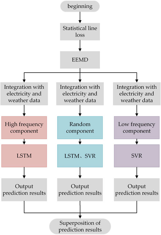
FIGURE 5. Prediction flowchart of EEMD–LSTM–SVR.

5 Simulation Experiment and Data Analysis

The target value of the dataset in this article is the statistical line loss of the UHV transmission line from 27 September 2017 to 29 April 2019, which is updated daily with 509 data points. The first 400 days are used as training data to predict the statistical line losses for the next 3 months (from 25 December 2018 to 15 April 2019). The historical data of statistical line loss are shown in Figure 6, which has a strong nonlinear characteristic. The line loss sequence jitter is very sharp, with two peaks, the first in July and August 2018 and the second in December 2018. The residential load peaks in summer and winter and the power that needs to be transmitted by the high voltage transmission lines increase accordingly, so the losses also peak.

FIGURE 6

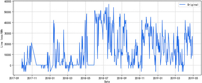
FIGURE 6. Historical data of statistical line loss.

In this article, EEMD is used to decompose the statistical line loss, as shown in Figure 7. The figure contains the original statistical line loss and the decomposed eight IMFs. After decomposition, IMF1∼IMF2 fluctuate frequently and are called high-frequency components. IMF3∼IMF5 show strong randomness. IMF6∼IMF7 have certain periodicity and linear characteristics and belong to low-frequency components. IMF8 is the residual.

FIGURE 7

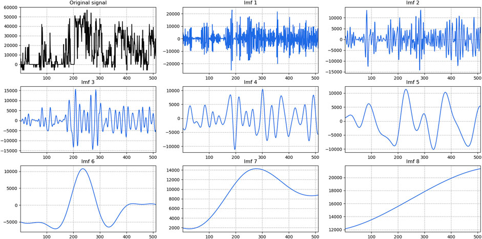
FIGURE 7. EEMD decomposition renderings.

5.1 EEMD–LSTM–SVR With Cross-Validation and Grid Search Tuning

After EEMD, each IMF needs to be learned and predicted separately. Cross-validation is often applied in the process of building prediction models and validating model parameters. Specifically, existing datasets are reused and sliced using different ways, and then various combinations of training and validation sets are fed into the model, where the training set is used for model training and the validation set is excellent for validating the model. With different partitioning methods, the data that are used as training at one time may become samples in the test set in the next iteration, thus achieving cross-validation. As for time-series data, incremental window cross-validation or fixed window cross-validation can be used to ensure temporal integrity as well as to prevent future data leakage. Grid search tuning is an automatic tuning method, where the optimal parameters are derived by specifying a prediction model with a given parameter tuning range. This method is more advantageous when applied to small datasets, and the sklearn library provides a function GridSearchCV specifically for debugging parameters (Bokde et al., 2020; Liu et al., 2021).

Applying cross-validation to a small sample set maximizes the sample information. Also, by repeatedly applying the trained model to new data, the overfitting can be reduced to a certain extent, thus increasing the model’s robustness. After grid tuning, the model’s training speed and prediction accuracy have been greatly improved.

After the decomposition of the statistical line loss, the processing for the different IMFs is as follows, and the flowchart is shown in Figure 8.

• First, choose a suitable predicting model. This article has two alternative predicting models: LSTM and SVR.

• Then, incremental division is performed for each IMF. The last 3 months of data were taken out. This part will not participate in the training process because in predicting practical applications, this part is unknown. It is exactly the value we need to predict. The incremental division is used for the first 400 days of data, and the number of increments is set to 6. Figure 9 shows the schematic.

• The grid search is performed for six different combinations of datasets, where the LSTM is adjusted for the number of hidden layer cells and the number of batches fed into the model each time. Specifically, the number of cells is first adjusted to determine the approximate range in intervals of 10 from 10 to 100, and then the best parameters are searched for in the reduced range in units of 1. The judging criterion is the box plot of the validation loss. After determining the number of cells, it is substituted into the model, and the same steps are used to search for the optimal n_batch. The other parameters of the LSTM are set as follows: the optimizer is Adam, the activation method of the fully connected layer is linear, the loss evaluation indicator is MSE, and the epochs-num in each iteration is 500.

• SVR mainly adjusts the kernel function and penalty factor C. The kernel function includes rbf, linear, and poly. The penalty factor C is tuned in the range from 0.01 to 100 in an isometric series with a total of 10 elements.

• After selecting a suitable prediction model for each IMF and performing cross-validation and grid tuning, the best parameters are used for prediction. The prediction results are superimposed to obtain the final statistical line loss prediction.

FIGURE 8

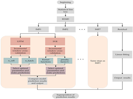
FIGURE 8. Flowchart of incremental cross-validation and grid search.

FIGURE 9

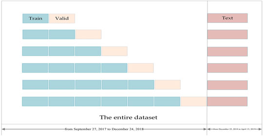
FIGURE 9. Schematic diagram of incremental cross-validation of time-series data.

Among the eight IMFs, IMF1, IMF2, IMF4, and IMF5 are predicted by LSTM, and IMF3, IMF6, and IMF7 are predicted by SVR. IMF8 is the residual quantity, which can be derived using linear fitting and does not require specialized prediction. For the aforementioned incremental cross-validation and grid research, IMF4 is selected for a detailed explanation.

Component 4 is a random IMF, and the first step is to predict it using LSTM. The first 400 days of data are taken as the training set and the last 3 months of data as the test set. The test set is not involved in training throughout to avoid future data leakage during the prediction process. The training set is then divided incrementally, with the first iteration using the first 66 days of data and then using the next 66 days for validation; the second iteration adds the previous validation set to the training set, using the first 132 days of data for training and the immediately following 66 days of data for validation and incrementally cross-validating like this. After advancing six times, all the data in the training set are well trained and learned.

The combination of cross-validation and grid search is then trained by taking cell values from 10 to 100 in units of 10, and the validation process is performed six times, each time a new cell value is entered. Figure 10A shows the box plot of six times cross-validation for each cell value, and the overall loss level in the region from 50 to 70 is the smallest. Then, the cell search is carried out again in 50 to 70 in units of 1. As shown in box Figure 10B, when the cell is 52, the box figure is the shortest, and the outlier points are evenly distributed. The n_cell in the model is set to 52, and the aforementioned steps are repeated to continue the optimization search for n_batch, as shown in Figure 11. First, the range from 10 to 100 is narrowed to 10 to 30, and then the search is conducted one by one, and the best performance is achieved when the n_batch is 14.

FIGURE 10

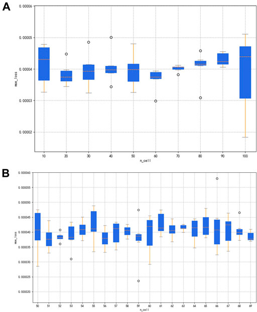
FIGURE 10. Box plots of feature 4 for incremental cross-validation and grid search using LSTM. (A) Optimization of n_cell from 10 to 100 in units of 10; and (B) optimization of n_cell from 50 to 70 in units of 1.

FIGURE 11

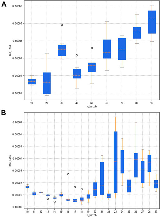
FIGURE 11. Box plot of feature 4 for incremental cross-validation and grid search using LSTM. (A) Optimization of n_batch in units of 10 from 10 to 100; and (B) optimization of n_batch in units of 1 from 50 to 70.

The parameters after the optimization are brought into the model, and the test set is input into the model for prediction. Figure 12 shows the comparison between the prediction results without optimization and after the optimization. It can be seen that the delay of the prediction curve is improved by adjusting n_cell, and the smoothness of the prediction curve is improved by adjusting n_batch after using cross-validation tuning. The root-mean-square error of the prediction curve is 808.533 MWH before the adjustment and 171.205 MWH after the adjustment, and the root-mean-square error decreases 78.83% from the original one.

FIGURE 12

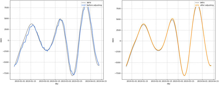
FIGURE 12. Comparison of prediction results before and after incremental cross-validation of the LSTM model.

The second part is the prediction of IMF4 using SVR, still using incremental cross-validation, and the kernel function and penalty factor C are adjusted. The comparison graph of prediction results before and after adjustment is shown in Figure 13. The root-mean-square error of prediction before adjustment is 833.325 MWH, and after adjustment, the root-mean-square error of prediction is 832.195 MWH, and the root-mean-square error has decreased by 0.1% from the original one. Compared with the LSTM model, the prediction results are poor and time-shifted. Therefore, the LSTM was finally selected for the prediction of IMF4.

FIGURE 13

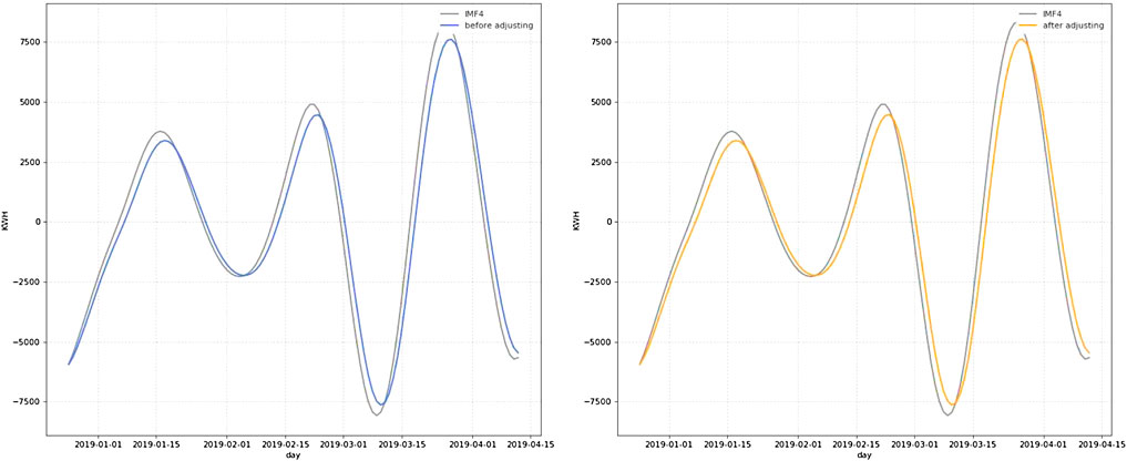
FIGURE 13. Comparison of prediction results before and after incremental cross-validation of the SVR model.

After performing the aforementioned operations on each IMF, the final prediction plot is shown in Figure 14. According to the different characteristics of IMFS, the high-frequency components IMF1 and 2 are predicted by LSTM. The overall results of IMF1 and 2 are good, but due to the strong jitteriness of the high-frequency components, it can be seen in the figure that the predictions are poor in some tip parts. However, the time-shiftedness that would exist in time series prediction has been resolved by incremental cross-validation. Among the stochastic components, IMF3 is better predicted by SVR, while IMF4 and 5 are better predicted by LSTM. The IMF3 prediction has a slight time-shift, but the SVR training is fast, so it achieves a very good prediction in aggregate. The IMF4 and 5 prediction is an exact match to the actual value. SVR predicts the low-frequency components IMF6 and 7 due to their regularity, to speed up the model training. The predictions of IMF6 and 7 have a slight time-shift, but the overall prediction is excellent. IMF8 is a residual series with very strong regularity, and a great prediction can be obtained with a linear fit. Figure 15 is the prediction results of EEMD–LSTM–SVR with or without cross-validation, from which we can see that the tip of the red curve is more moderate and closer to the real line loss. The blue curve does not use incremental cross-validation which tends to overfit in the tip part of the curve and has some time-shift. This demonstrates that the use of incremental cross-validation and grid search can effectively prevent model overfitting and improve model prediction accuracy.

FIGURE 14

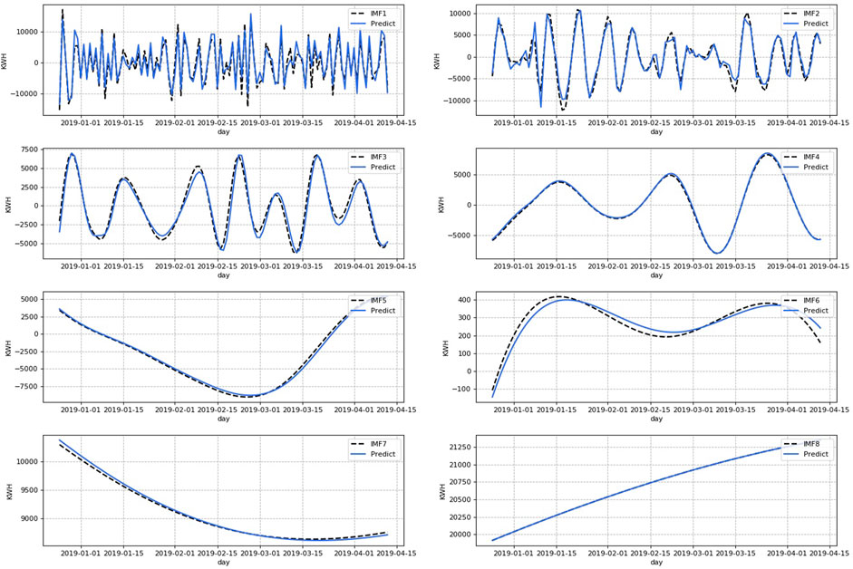
FIGURE 14. Prediction results of each IMF component using EEMD–LSTM–SVR.

FIGURE 15

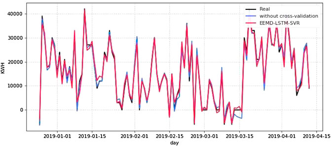
FIGURE 15. Prediction results of EEMD–LSTM–SVR with or without cross-validation.

5.2 Benchmark Models

For energy managers and power operators, accurate line loss forecasting is imperative to reduce the uncertainty of statistical line losses. The strong jitteriness of statistical line losses poses a challenge to accurate forecasting. In this article, we decompose the line loss by EEMD. As a preprocessing technique, EEMD decomposes the statistical line loss into eight subseries of different frequencies and feeds the decomposition results into various models for learning prediction. The statistical line loss is originally strongly uncertain and jittery, while the decomposed IMF shows regularity and smoothness, which help the model learning, thus improving the prediction accuracy.

In this section, independent LSTM and SVR are used for prediction as benchmark models. Then, they are compared with EEMD–LSTM–SVR, EEMD–LSTM, and EEMD–SVR. The difference between the models is the use of a combined predictive model and EEMD decomposition. In order to verify the ability of EEMD to help the model learn target value features and where the combined model outperforms the independent model, predictive performance was assessed on daily predictions. Since the target values are significantly greater than zero in both cases, the mean absolute performance error (MAPE) is an appropriate selection for measuring the forecasting error.

The MAPE is defined as follows:

$MAPE=\frac{100\%}{n}{\displaystyle \sum _{i=1}^n\left|\frac{y_i-{\widehat{y}}_i}{y_i}\right|},(24)$

where $N$ denotes the number of forecasted points, $y_i$ denotes the actual value, and ${\widehat{y}}_i$ denotes the forecasted value.

In order to evaluate the prediction results of various models more comprehensively, the following five evaluation indicators are also taken into consideration.

Symmetric mean absolute percentage error:

$SMAPE=\frac{100\%}{n}{\displaystyle \sum _{i=1}^n\frac{\left|{\widehat{y}}_i-y_i\right|}{\left(\left|{\widehat{y}}_i\right|+\left|y_i\right|\right)/2}}.(25)$

Mean absolute error:

$MAE=\frac{1}{n}{\displaystyle \sum _{i=1}^n\left|{\widehat{y}}_i-y_i\right|}.(26)$

Mean square error:

$MSE=\frac{1}{n}{\displaystyle \sum _{i=1}^n{\left({\widehat{y}}_i-y_i\right)}^2}.(27)$

Root mean square error:

$RMSE=\sqrt{\frac{1}{N}{\displaystyle \sum _{i=1}^n{\left( y_i-{\widehat{y}}_i\right)}^2}}.(28)$

R-square:

$R^2=1-\frac{{\displaystyle \sum _{i=1}^n{\left({\widehat{y}}_i-y_i\right)}^2}}{{\displaystyle \sum _{i=1}^n{\left({\overline{y}}_i-y_i\right)}^2}}.(29)$

To ensure the reliability of the comparison results, all five models use incremental cross-validation and grid search. The differences among the five models are whether to use EEMD and which prediction algorithm to use. The prediction results of each model are shown in Figure 16. The subplots one to five show the prediction of the five models individually, and the last subplot shows the comparison of the five models. It can be found that the prediction curves still show strong volatility overall.

FIGURE 16

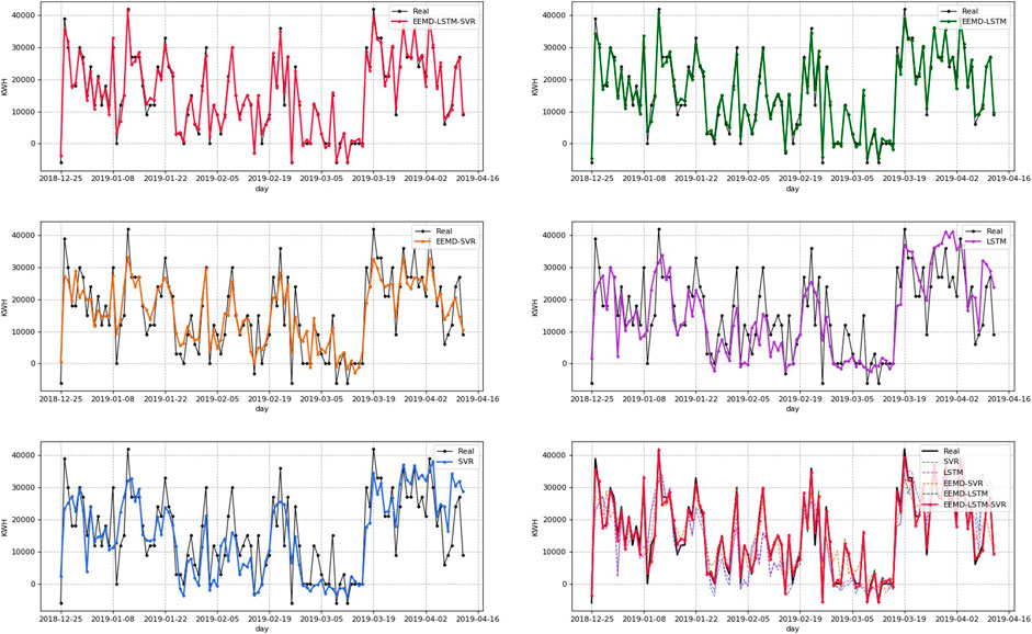
FIGURE 16. Prediction results of each model. The order is EEMD–LSTM–SVR, EEMD–LSTM, EEMD–SVR, LSTM, and SVR. The final one is a comprehensive comparison.

As can be seen in Figure 16, using EEMD–LSTM has been able to achieve an excellent prediction with an R² of 0.9796, but using the combined model EEMD–LSTM–SVR was able to improve MAPE by 2.2% and MAE by 265.2 kwh. The case illustrates that the combined model can indeed effectively improve the model prediction accuracy. Among them, the trends of the prediction curves of EEMD–LSTM–SVR and EEMD–LSTM are basically consistent with the actual values, and the EEMD–LSTM–SVR model has the best prediction effect, the most accurate tip fitting, and the closest to the real value, indicating that EEMD–LSTM–SVR has the best prediction result. The prediction effect of EEMD–LSTM is close to that of EEMD–LSTM–SVR, but the fit at the tip is slightly worse and the prediction accuracy is slightly lower. Compared with the EEMD–LSTM model, the prediction accuracy of the EEMD–SVR model is greatly reduced and not only appears time-shifted but also biased to predict the mean at the tip, indicating that the prediction effect of the machine learning model SVR is worse than the learning ability of the deep learning model LSTM. The LSTM model is more advantageous in dealing with time series and high-frequency components. The LSTM and SVR without EEMD modal decomposition have the worst prediction effect, with obvious time-shiftedness, and the prediction result tends to the average trend of the curve.

The model accuracy evaluation is shown in Table 3. The table shows the values of the corresponding evaluation metrics for the five models: MAPE%, SMAPE%, MAE, MSE, RMSE, and R². EEMD–LSTM–SVR performs best in all metrics. R² is as high as 0.9878, MAPE% is only 6.4736, and MAE is only 1.0844 MW. EEMD–LSTM is closer to EEMD–LSTM–SVR metrics, while EEMD–SVR has a disconnected decline in metrics. The individual prediction models LSTM and SVR, on the other hand, have the worst performance in all indicators.

TABLE 3

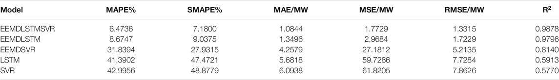
TABLE 3. Accuracy evaluation table of each model.

The prediction effect of EEMD–LSTM is significantly better than that of EEMD–SVR. Reflected in the evaluation indexes, the R² of EEMD–LSTM is 0.9796 and that of EEMD–SVR is 0.8140; the MAPE of EEMD–LSTM is reduced by 23.16 compared with that of EEMD–SVR; the MAE of EEMD–LSTM is reduced by 68.3% compared with that of EEMD–SVR; MSE of EEMD–LSTM is reduced by 89.08% compared to that of EEMD–SVR. The difference between LSTM and SVR models is not large. The R² of LSTM is 0.5913, and the R² of SVR is 0.5770. The reason why the EEMD–LSTM model will outperform EEMD–SVR in all evaluation indexes is due to the strong learning ability of LSTM for high-frequency components, and the decomposition of regular quantities by EEMD further strengthens the learning capability. It is proved that LSTM, as a deep learning model, further strengthens the learning ability for high-frequency components after EEMD decomposition of target values.

In order to show the prediction results more intuitively, five indicators are used to describe the prediction results of the five models, and the following conclusions can be drawn from the comprehensive evaluation results:

1. The prediction effect of the combined model is much better than that of the independent model. The indicators of the EEMD–LSTM–SVR model in the comprehensive evaluation Table 3 are significantly smaller than those of EEMD–LSTM and EEMD-–SVR. Independent models may have unique advantages in one aspect, but they also have corresponding disadvantages. For example, the SVR model is relatively simple and fast to train, but it is often difficult to learn the pattern when the target curve changes drastically, resulting in poor prediction results. The LSTM, on the other hand, has advantages in dealing with frequently changing time series, but the training time is longer. The combined model combines the advantages of both algorithms, which can speed up the model training and ensure the prediction accuracy. Therefore, when performing time series prediction, modal decomposition of the target curve and then adopting the combined model prediction can effectively improve the prediction performance.

2. The EEMD–LSTM model predicts better than the EEMD–SVR model, and the LSTM model predicts better than the SVR. As can be seen from Table 3, the MAPE% value of the EEMD–SVR model is almost four times that of the EEMD–LSTM model. Influenced by the simpler structure of the SVR model, the SVR model has a weaker learning ability when dealing with some complex change trends. The machine learning model SVR is not so good at predicting high-frequency components compared to the deep learning model LSTM. The EEMD–SVR model performs significantly better than the SVR but still has a large gap with the EEMD–LSTM model. LSTM, as a deep learning algorithm specialized in processing temporal data, is indeed more advantageous.

3. EEMD can significantly improve model learning and prediction capabilities. EEMD–LSTM improves MAPE by 32.72% on the basis of LSTM, and EEMD–SVR improves MAPE by 11.16% on the basis of SVR, indicating that modal decomposition of line loss helps the model to learn its nonlinear characteristics and performs better in prediction.

4. The EEMD–LSTM–SVR model has the best predictive performance. The MAE, MSE, and RMSE of the EEMD–LSTM–SVR model are 1.0844, 1.7729, and 1.3315 MW, respectively. Only one-fifth of that of the EEMD–SVR model indicates that the EEMD–LSTM–SVR model has the best prediction performance with less discrete results and better single-point prediction. The MAPE% and SMAPE% of the EEMD–LSTM–SVR model are 6.4736 and 7.18, respectively. At least 2.2011 and 1.8575 lower than the other four models, indicating that the EEMD–LSTM–SVR model has less prediction bias and higher reliability of prediction results. The R² of the EEMD–LSTM–SVR model is close to 1, which demonstrates that the EEMD–LSTM–SVR model has a better overall fitting degree.

In conclusion, EEMD–LSTM–SVR achieves the accurate prediction of line loss of UHV transmission lines, which has important scientific and practical significance. 1) The case shows that EEMD is suitable for dealing with strong jittering target values. It solves the problem of difficult nonlinear target prediction and meets the engineering requirements. 2) Accurate line loss prediction improves energy utilization efficiency and can effectively predict power theft as well as extreme weather loss, which improves the economic efficiency of power grid companies. 3) Stable and reliable statistical line loss prediction is an important basis for ensuring the operational safety of the UHV transmission system, reasonable power generation planning by power generation departments, and timely grid dispatch. Accurate line loss prediction is helpful for grid maintenance personnel to arrange timely maintenance, reduce the impact of line loss to the power system, and ensure safe and stable operation of the power system. 4) The EEMD–LSTM–SVR prediction model can also be used for the prediction of other clean energy sources, such as reducing wind power uncertainty and improving the accuracy of photovoltaic power generation prediction, and this model provides a new guidance method for the production and utilization of clean energy.

6 Concluding Remarks

In this work, we construct trend and curve characteristics of time series data and other methods to expand the dimension of input data, which can more finely describe the running condition of the line with different line loss values. Then, we proposed a hybrid methodology to combine EEMD with SVR and, in particular LSTM, for predicting daily UHV line loss. First, the line loss is decomposed into trend components and random and high-frequency IMFs. The addition of EEMD can help the model learn data features better. The combination of artificial intelligence algorithm LSTM and machine learning SVR can not only further improve model calculation accuracy but also further save model training time.

Compared with several models, the actual electric line loss data were used to verify the model. The results show that

1. Compared with EEMD–SVR, the MAE of EEMD–LSTM–SVR decreased by 74.53%, RMSE decreased by 74.46%, and MAPE% decreased by 25.37. Compared with EEMD–LSTM, EEMD–LSTM–SVR reduced the MAE by 19.65%, RMSE by 22.72%, and MAPE% by 2.2. It shows that using machine learning to predict low-frequency components and applying artificial intelligence algorithms to predict high-frequency components can greatly improve prediction accuracy. That is, the combined model performs better than the individual models.

2. Compared with SVR, the MAE of EEMD–SVR decreased by 30.13%, RMSE decreased by 33.69%, and MAPE% decreased by 11.16. Compared with LSTM, the MAE of EEMD-LSTM decreased by 76.25%, RMSE decreased by 77.71%, and MAPE% decreased by 32.72. The difference between them is whether the line loss is decomposed by EEMD. The results show that EEMD of line loss series can effectively separate the complex information contained in the original series and then predict each component separately, which helps to improve the prediction accuracy of the model and the prediction ability of the line loss trend. In addition, using EEMD can also reduce the model computation time.

3. EEMD–LSTM–SVR has the highest R-square, of which is as high as 0.9878. The mean R-square of the model with EEMD reached 0.9271, while the mean R-square of the model without EEMD was only 0.5841. It indicates that this method has good application prospects for line loss forecasting. The robustness of the model is also reliably guaranteed by using incremental cross-validation and grid search.

The main contributions of this article are:

• Previous studies, including various machine learning models and deep learning models, have been shown to be useful for line loss prediction. However, changes in the weights and threshold parameters of neural networks can affect the results. The simple structure of machine learning models can hardly cope with high-frequency components, and various single models are poor at predicting strong jitteriness curves due to their own drawbacks. On the other hand, the application of combinatorial models relies on modal decomposition methods. To this end, a new intelligent prediction method, EEMD–LSTM–SVR, is proposed, and parameter optimization using incremental cross-validation and grid search is performed to improve the prediction accuracy.

• The research results show that EEMD–LSTM–SVR has better prediction results. The R² of EEMD–LSTM–SVR is closer to 1, which proves the superiority and reliability of the EEMD–LSTM–SVR model.

• The model can accurately predict the statistical line loss of the UHV transmission system, which is helpful to predict the transmission line loss, take corresponding maintenance or dispatching measures in time, and reduce the impact of unstable power supply quality on the grid. Meanwhile, the model proposed in this article can also be used for the prediction of other clean energy sources, which provides new guidance for reducing CO₂ emissions.

In the future study, the model parameter optimization algorithm can be replaced to reduce the overfitting and time shift of the prediction results and further improve the model training speed or try clustering algorithm to cluster the line losses of the same scenarios and input the typical scenarios into the model for learning, to further improve the model prediction accuracy. The algorithm can also be explored to be applied to other time series (e.g., wind power data, and PV data).

Data Availability Statement

The original contributions presented in the study are included in the article/Supplementary Material; further inquiries can be directed to the corresponding author.

Author Contributions

CD and YZ carried out the concepts, design, definition of intellectual content, literature search, data acquisition, data analysis, and manuscript preparation. CD provided assistance for data acquisition, data analysis, and statistical analysis. YZ carried out literature search, data acquisition, and manuscript editing. ZW and QD performed manuscript review. All authors have read and approved the content of the manuscript and have made substantial contributions to all of the following: 1) the conception and design of the study, or acquisition of data, or analysis and interpretation of data; 2) drafting the manuscript or revising it critically for intellectual content; and 3) final approval of the version to be submitted.

Funding

This research received no external funding.

Conflict of Interest

The authors declare that the research was conducted in the absence of any commercial or financial relationships that could be construed as a potential conflict of interest.

Publisher’s Note

All claims expressed in this article are solely those of the authors and do not necessarily represent those of their affiliated organizations, or those of the publisher, the editors, and the reviewers. Any product that may be evaluated in this article, or claim that may be made by its manufacturer, is not guaranteed or endorsed by the publisher.

References

Agami, R. T. (2011). “Analysis of Time Series Data,” in Applied Data Analysis and Modeling for Energy Engineers and Scientists (Boston, MA: Springer). doi:10.1007/978-1-4419-9613-8_9

CrossRef Full Text | Google Scholar

Alamin, Y. I., Anaty, M. K., Álvarez Hervás, J. D., Bouziane, K., Pérez García, M., Yaagoubi, R., et al. (20202020). Very Short-Term Power Forecasting of High Concentrator Photovoltaic Power Facility by Implementing Artificial Neural Network. Energies 13, 3493. doi:10.3390/en13133493

CrossRef Full Text | Google Scholar

Audinet, P., Amado, J. C., and Rabb, B. (2014). Climate Risk Management Approaches in the Electricity Sector: Lessons from Early Adapters. New York, NY: Weather Matters for EnergySpringer.

Google Scholar

Baran, I., Leonida, T., and Sidea, D. (2013). Using Numerical Weather Forecast to Predict Power Losses on Transmission Lines. Int. Symp. Electr. Elect. Eng. (Iseee), 1–8. doi:10.1109/iseee.2013.6674326

CrossRef Full Text | Google Scholar

Bokde, N. D., Feijoo, A., Al-Ansari, N., and Yaseen, Z. M. (2019). A Comparison between Reconstruction Methods for Generation of Synthetic Time Series Applied to Wind Speed Simulation. IEEE Access 7, 135386–135398. doi:10.1109/ACCESS.2019.2941826

CrossRef Full Text | Google Scholar

Bokde, N. D., Tranberg, B., and Andresen, G. B. (2021). Short-term CO2 Emissions Forecasting Based on Decomposition Approaches and its Impact on Electricity Market Scheduling. Appl. Energ. 281, 116061. doi:10.1016/j.apenergy.2020.116061

CrossRef Full Text | Google Scholar

Bokde, N. D., Yaseen, Z. M., and Andersen, G. B. (2020). ForecastTB-An R Package as a Test-Bench for Time Series Forecasting-Application of Wind Speed and Solar Radiation Modeling. Energies 13, 2578. doi:10.3390/en13102578

CrossRef Full Text | Google Scholar

Bokde, N., Feijóo, A., Villanueva, D., and Kulat, K. (2019). A Review on Hybrid Empirical Mode Decomposition Models for Wind Speed and Wind Power Prediction. Energies 12, 254. doi:10.3390/en12020254

CrossRef Full Text | Google Scholar

Chang, W.-Y. (2013). Short-Term Wind Power Forecasting Using the Enhanced Particle Swarm Optimization Based Hybrid Method. Energies 6, 4879–4896. doi:10.3390/en6094879

CrossRef Full Text | Google Scholar

Chen, T., Song, M., Hui, H., and Long, H. (2021). Battery Electrode Mass Loading Prognostics and Analysis for Lithium-Ion Battery–Based Energy Storage Systems. Front. Energ. Res. 9, 543. doi:10.3389/fenrg.2021.754317

CrossRef Full Text | Google Scholar

Daochun Huang, D., Yinbiao Shu, Y., Jiangjun Ruan, J., and Yi Hu, Y. (2009). Ultra High Voltage Transmission in China: Developments, Current Status and Future Prospects. Proc. IEEE 97 (3), 555–583. doi:10.1109/JPROC.2009.2013613

CrossRef Full Text | Google Scholar

Deng, D., Li, J., Hu, W., Huang, Q., Xu, S., and Xu, D. (2019). Line Loss Association and Prediction Model Based on Deep Learning. IEEE Innovative Smart Grid Technologies - Asia, 865–869.

Google Scholar

Huang, S., Ye, Z., Liu, Y., Yan, X., Liu, C., Li, Y., et al. (2021). Effects of the Rainfall Rate on corona Onset Voltage Gradient of Bundled Conductors in Alternating Current Transmission Lines in High-Altitude Areas. Electr. Pow Syst. Res. 2021200, 107461.

Google Scholar

Jindal, A., Dua, A., Kaur, K., Singh, M., Kumar, N., and Mishra, S. (2016). Decision Tree and SVM-Based Data Analytics for Theft Detection in Smart Grid. IEEE Trans. Ind. Inf. 12, 1005–1016. doi:10.1109/TII.2016.2543145

CrossRef Full Text | Google Scholar

Khan, A. H., and Islam, M. D. (2019). Prediction of thermal Efficiency Loss in Nuclear Power Plants Due to Weather Conditions in Tropical Region. Energ. Proced. 160, 84–91. doi:10.1016/j.egypro.2019.02.122

CrossRef Full Text | Google Scholar

Li, G., Wang, H., Zhang, S., Xin, J., and Liu, H. (2019). Recurrent Neural Networks Based Photovoltaic Power Forecasting Approach. Energies 12, 2538. doi:10.3390/en12132538

CrossRef Full Text | Google Scholar

Li, Q., Li, P., Zhang, Q., Ren, W., Cao, M., and Gao, S. (2011). Icing Load Prediction for Overhead Power Lines Based on SVM. In Proceedings of 2011 International Conference on Modelling. Shanghai, China: Identification and Control, 104–108. doi:10.1109/icmic.2011.5973684

CrossRef Full Text | Google Scholar

Liang, X., Li, S., Gao, Y., Su, Z., and Zhou, J. (2020). Improving the Outdoor Insulation Performance of Chinese EHV and UHV AC and DC Overhead Transmission Lines. IEEE Electr. Insul. Mag. 36 (4), 7–25. doi:10.1109/MEI.2020.9111096

CrossRef Full Text | Google Scholar

Liu, K., Zhou, H., Yang, Z., and Qu, F. (2011). “Application of BP Neural Network for Line Losses Calculation Based on Quantum Genetic Algorithm,” in 2011 Fourth International Symposium on Computational Intelligence and Design, 3–7. doi:10.1109/ISCID.2011.9

CrossRef Full Text | Google Scholar

Liu, Y., Li, L., Tseng, M. L., Lim, M. K., and Helmi Ali, M. (2021). Optimal Scheduling of Combined Cooling, Heating, and Power Microgrid Based on a Hybrid gray Wolf Optimizer. J. Ind. Prod. Eng. doi:10.1080/21681015.2021.1974963

CrossRef Full Text | Google Scholar

Liu, Z.-F., Li, L.-L., Tseng, M.-L., Tan, R. R., and Aviso, K. B. (2019). Improving the Reliability of Photovoltaic and Wind Power Storage Systems Using Least Squares Support Vector Machine Optimized by Improved Chicken Swarm Algorithm. Appl. Sci. 9, 3788. doi:10.3390/app9183788

CrossRef Full Text | Google Scholar

Liu, Z.-F., Luo, S.-F., Tseng, M.-L., Liu, H.-M., Li, L., and Hashan Md Mashud, A. (2021). Short-term Photovoltaic Power Prediction on Modal Reconstruction: A Novel Hybrid Model Approach. Sustainable Energ. Tech. Assessments 45, 101048. doi:10.1016/j.seta.2021.101048

CrossRef Full Text | Google Scholar

Min, T., Xinghua, W., Qing, L., Lexin, G., Tao, Y., and Yongkun, F. (2015). Application of Support Vector Machine Based on Particle Swarm Optimization in Low Voltage Line Loss Prediction. doi:10.2991/jimet-15.2015.35

CrossRef Full Text | Google Scholar

Miraftabzadeh, S. M., Longo, M., Foiadelli, F., Pasetti, M., and Igual, R. (2021). Advances in the Application of Machine Learning Techniques for Power System Analytics: A Survey. Energies 14, 4776. doi:10.3390/en14164776

CrossRef Full Text | Google Scholar

Mohd Zainuddin, N., Abd. Rahman, M. S., Ab. Kadir, M. Z. A., Nik Ali, N. H., Ali, Z., Osman, M., et al. (2020). Review of Thermal Stress and Condition Monitoring Technologies for Overhead Transmission Lines: Issues and Challenges. IEEE Access 8, 120053–120081. doi:10.1109/ACCESS.2020.3004578

CrossRef Full Text | Google Scholar

Peng, H., Wen, W., Tseng, M. L., and Li, L. (2021). A Cloud Load Forecasting Model with Nonlinear Changes Using Whale Optimization Algorithm Hybrid Strategy. Soft Comput. 25. doi:10.1007/s00500-021-05961-5

CrossRef Full Text | Google Scholar

Rudolf, L., Kral, V., and Bernat, M. (2019). Calculation of Losses in Transmission System in Dependence on Temperature and Transmitted Power. Int. Scientific Conf. Electric Power Eng. (Epe), 1–5. doi:10.1109/epe.2019.8777974

CrossRef Full Text | Google Scholar

Sahlin, J., Eriksson, R., Ali, M. T., and Ghandhari, M. (2017). Transmission Line Loss Prediction Based on Linear Regression and Exchange Flow Modelling. IEEE Manchester Power Tech., 1–6. doi:10.1109/ptc.2017.7980810

CrossRef Full Text | Google Scholar

Savian, F. d. S., Siluk, J. C. M., Garlet, T. B., do Nascimento, F. M., Pinheiro, J. R., and Vale, Z. (2021). Non-technical Losses: A Systematic Contemporary Article Review. Renew. Sust. Energ. Rev. 147, 111205. doi:10.1016/j.rser.2021.111205

CrossRef Full Text | Google Scholar

Simões, P., Souza, R., Calili, R., and Pessanha, J. (2020). Analysis and Short-Term Predictions of Non-technical Loss of Electric Power Based on Mixed Effects Models. Socio-econ Plan. SCI. 71, 100804.

Google Scholar

Song, Y. (2019). “Safety Management Principles in Electric Power Industry Based on Human Factors,” in Advances in Artificial Intelligence, Software and Systems Engineering. AHFE 2018. Advances in Intelligent Systems and Computing. Editor T. Ahram (Cham: Springer), 787. doi:10.1007/978-3-319-94229-2_52

CrossRef Full Text | Google Scholar

Sun, W., Zhang, H., Tseng, M. L., Zhang, W., and Li, X. (2021). Hierarchical Energy Optimization Management of Active Distribution Network with Multi-Microgrid System. J. Ind. Prod. Eng.

Google Scholar

Tao, X., Yu, M., Zhu, J., Yu, C., and Zhang, S. (2019). Prediction of Zone Area Line Loss Anomalies Based on PCA and Improved CHAID Decision Tree. 34rd Youth Academic Annual Conference of Chinese Association of Automation, 221–226.

Google Scholar

Ti, Z., Deng, X. W., and Zhang, M. (2021). Artificial Neural Networks Based Wake Model for Power Prediction of Wind Farm. Renew. Energ. 172, 618–631. doi:10.1016/j.renene.2021.03.030

CrossRef Full Text | Google Scholar

Tulensalo, J., Seppänen, J., and Ilin, A. (2020). An LSTM Model for Power Grid Loss Prediction. Electric Power Syst. Res. 189, 106823. doi:10.1016/j.epsr.2020.106823

CrossRef Full Text | Google Scholar

Wang, W., Shi, X., Li, M., Cheng, X., Liu, X., Huo, C., et al. (2020). “Research on Theoretical Line Loss Calculation Analysis and Loss Reduction Measures of Main Network Based on Multiple Factors,” in Recent Trends in Intelligent Computing, Communication and Devices. Advances in Intelligent Systems and Computing. Editors V. Jain, S. Patnaik, F. Popeniu Vlădicescu, and I. Sethi (Singapore: Springer), 1006. doi:10.1007/978-981-13-9406-5_107

CrossRef Full Text | Google Scholar

Wen, S., Wang, Y., Tang, Y., Xu, Y., Li, P., and Zhao, T. (2019). Real-Time Identification of Power Fluctuations Based on LSTM Recurrent Neural Network: A Case Study on Singapore Power System. IEEE. T. Ind. Iuform. 15 (9), 5266–5275. doi:10.1109/TII.2019.2910416

CrossRef Full Text | Google Scholar

Wu, Q., and Peng, C. (2016). Wind Power Generation Forecasting Using Least Squares Support Vector Machine Combined with Ensemble Empirical Mode Decomposition, Principal Component Analysis and a Bat Algorithm. Energies 9, 261. doi:10.3390/en9040261

CrossRef Full Text | Google Scholar

Xia, Y., Zhao, J., Ding, Q., and Jiang, A. (2021). Incipient Chiller Fault Diagnosis Using an Optimized Least Squares Support Vector Machine with Gravitational Search Algorithm. Front. Energ. Res. 9, 717. doi:10.3389/fenrg.2021.755649

CrossRef Full Text | Google Scholar

Xin, K., Yang, Y., and Chen, F. (2002). An Advanced Algorithm Based on Combination of GA with BP to Energy Loss of Distribution System. Proc. CSEE 22 (2), 79–82.

Google Scholar

Yan, X., Rui, Z., Zhao, J., Zhao, Y. D., Wang, D., and Yang, H. (2016). Assessing Short-Term Voltage Stability of Electric Power Systems by a Hierarchical Intelligent System. IEEE. T. Neur. Net. Lear. 27 (8), 1686–1696.

Google Scholar

Yao, M., Zhu, Y., Li, J., Wei, H., and He, P. (2019). Research on Predicting Line Loss Rate in Low Voltage Distribution Network Based on Gradient Boosting Decision Tree. Energies 12, 2522. doi:10.3390/en12132522

CrossRef Full Text | Google Scholar

Zhang, J., Williams, S. O., and Wang, H. (2018). Intelligent Computing System Based on Pattern Recognition and Data Mining Algorithms. Sust. Comput. Inform. Syst. 20, 192–202. doi:10.1016/j.suscom.2017.10.010

CrossRef Full Text | Google Scholar

Zheng, Q., Yan, P., Zareipour, H., and Niya, C. (2019). A Review and Discussion of Decomposition-Based Hybrid Models for Wind Energy Forecasting Applications. Appl. Energ. 235, 939–953.

Google Scholar

Zhong, X., Chen, J., Jiang, M., and Zheng, X. (2020). A Line Loss Analysis Method Based on Deep Learning Technique for Transformer District. Power Sys Techno 44 (02), 769–774.

Google Scholar

Zhou, F., Zhou, H., Yang, Z., and Yang, L. (2019). EMD2FNN: A Strategy Combining Empirical Mode Decomposition and Factorization Machine Based Neural Network for Stock Market Trend Prediction. Expent. Syst. Appl. 115, 136–151. doi:10.1016/j.eswa.2018.07.065

CrossRef Full Text | Google Scholar

Zhou, Q., Yu, K., Chen, X., and Liu, S. (2018). Calculation Method of the Line Loss Rate in Low-Voltage Transformer District Based on PCA and K-Means Clustering and Support Vector Machine. In International Conference on Power System Technology. Guangzhou, China: POWERCON, 4264–4271. doi:10.1109/POWERCON.2018.8601624

CrossRef Full Text | Google Scholar

Zhou, W., Li, Y., Guo, Y., Qiao, X., Mei, Y., and Deng, W. (2021). Daily Line Loss Rate Forecasting of a Distribution Network Based on DAE-LSTM. Power Syst. Prot. Control. 49 (17), 201483.

Google Scholar