Residential load forecasting based on electricity consumption pattern clustering

In order to reduce the peak load on the power grid, various types of demand response (DR) programs have been developed rapidly, and an increasing number of residents have participated in the DR. The change in residential electricity consumption behavior increases the randomness of electricity load power, which makes residential load forecasting relatively difficult. Aiming at increasing the accuracy of residential load forecasting, an innovative electricity consumption pattern clustering is implemented in this paper. Six categories of residential load are clustered considering the power consumption characteristics of high-energy-consuming equipment, using the entropy method and criteria importance though intercrieria correlation (CRITIC) method. Next, based on the clustering results, the residential load is predicted by the fully-connected deep neural network (FDNN). Compared with the prediction result without clustering, the method proposed in this paper improves the accuracy of the prediction by 5.21%, which is demonstrated in the simulation.

1 Introduction

Electric load forecasting can facilitate operation planning, revenue projection, electricity pricing, and energy trading for power systems. With the increase of residential load and the popularity of smart devices, residents have gradually become a target customer for demand response (DR) (Qian et al., 2019). Residential electricity consumption behavior, especially related to the high-energy-consuming equipment, can be changed for participation in DR, which leads to extra fluctuations in residential load. Except for the influence of DR, different energy-use habits result in a large difference in residential load power and relatively weak regularity (Lusis et al., 2017), which makes nowadays residential load forecasting more challenging (Hou et al., 2021; Liu et al., 2023).

In general, previous researches on residential load forecasting mainly depend on machine learning. Residential load data have been trained by machine learning to obtain a general load forecasting model in a recent study (Xie et al., 2020). Multi-layer long-short-term memory (LSTM) model, general back propagation neural network (Kong et al., 2017), and the hybrid modeling method combining both recurrent neural networks and Ornstein–Uhlenbeck process (Hua et al., 2018) have been applied to obtain accurate load prediction model. In recent years, personalized short-term load prediction for residential load has been achieved by transfer learning and meta-learning methods (Lee et al., 2021). A short-term load forecasting method based on deep neural network and iterative ResBlock (Hong et al., 2020) has been proposed to learn different electricity consumption behavior (Zhang et al., 2017). However, machine learning used in the majority of the aforementioned work requires a huge amount of data, such that a well-trained model can be built. Otherwise, insufficient data can lead to the problem of over-fitting, which means the difference between the error on the training set and the error on the test set is too large. Additionally, the forecasting accuracy of machine learning drops when the predicting a large fluctuation load.

Recently, the method of clustering first and predicting by machine learning later has shown an impressive success in overcoming the problem of over-fitting and enabling forecasting models to learn fluctuation characteristics among residential load (Zheng et al., 2019). Considering the similarity of the residential electricity consumption behavior within a certain area, the clustering algorithm can be used to aggregate the residents with similar electricity consumption characteristics, then the residential load is predicted via graph neural networks (Lin et al., 2021). The K-means clustering algorithm is introduced to cluster the load and the load is predicted based on deep learning. Evidence shows that under the premise of using the same algorithm, the accuracy of the prediction after clustering is generally higher than that of direct prediction (Liu et al., 2021). However, since these clustering algorithms manually select the number of clustering centers, these clustering methods cannot reflect sufficient information on residential load, which might lead to inaccurate clustering results. The machine learning algorithm trained based on these clustering results may be affected, when the power consumption of residents of one category in the clustered result data is very different from each other.

To further solve the issue of overfitting and to obtain more accurate clustering results, different methods have been proposed, which can be summarized into two main categories: proposing improved clustering algorithms (Du et al., 2019; Piao et al., 2014; Rodriguez et al., 2014) and proposing new clustering indicators. New clustering algorithms, such as distributed clustering method, have been proposed. A distributed clustering method is used to cluster the electric load in different regions and solve the dilemma of the high dimension of the input data (Wang et al., 2019). New clustering indicators are more capable of extracting the similarity of residential load effectively. Not only the original data of daily load, but also relevant indicators that can reflect the characteristics of load power consumption, such as daily peak-to-valley difference rate and peak power consumption rate, are considered in (Wang et al., 2020a). The empirical rank approximation method derived from singular value decomposition (SVD) is proposed, which extracts new load indicators of daily load curves for indirect clustering to ensure the efficiency and accuracy of the clustering process (Lu et al., 2019). According to the daily load curve, seven load characteristic indicators, e.g., daily load rate, peak load rate, and valley load rate, are extracted by entropy method (Cannas et al., 2021). Eight types of characteristic indicators are put forward by feature extraction of the daily load curve, and four conventional clustering algorithms are weighted based on the clustering effectiveness, which achieves an ensemble clustering method fully combining the advantages of different algorithms (Fujimoto et al., 2021). However, electricity consumption characteristics of residential high-energy-consuming equipment are not considered in the above study, nor is the impact of residents’ participation in DR considered. In addition, when the selection of indicators is subjective, there is a negative impact on the clustering effect. Thereby, it is necessary to screen and reasonably empower each clustering indicator.

Aiming at the accurate prediction of resident load and considering the effect of DR, the daily load curve of residents and the electricity consumption characteristics of equipment load are analyzed in this paper. Then, the characteristics are screened and weighted according to principal component analysis. Finally, a residential load forecasting method based on the combined weighted clustering method and FDNN is proposed. Our key contributions are.

1) The electricity consumption characteristics of high-energy-consuming equipment and the willingness of residents to participate in DR are considered to select clustering indicators, which helps to reflect the user’s electricity consumption habits. By principal component analysis, seven clustering indicators of the power consumption characteristics of high-energy-consuming equipment are chosen. These indicators have relatively low dimensions but can reflect sufficient information, cumulative contribution rate of which is as high as .980.

2) The clustering indicators are weighted based on the entropy method and CRITIC method, which can eliminate adverse effects caused by data level and subjective factors. By comparison with other methods, it is verified that the proposed clustering result is more accurate after employing the weighted clustering indicators by comparing value to the S_Dbw which is used to assess the effectiveness of clustering.

3) The residential load is predicted based on the clustering result and FDNN, and six types of resident load data obtained by clustering are trained separately, improving the prediction accuracy by 5.21% compared with the case without clustering.

The rest of the paper is organized as follows. In Section 2, cluster indicators of the daily load curve and power consumption characteristics of high-energy-consuming equipment are selected. In Section 3, the clustering model of the residents’ electricity mode based on the entropy method and CRITIC method is proposed. In Section 4, a residential load forecasting model based on residential electricity consumption pattern clustering and FDNN is established. In Section 5, the simulation results are presented, and conclusions are drawn in Section 6.

2 Cluster indicators selection based on daily load curve and high-energy-consuming equipment

Considering the continuous updating of various demand response projects, the willingness of residential users to participate in demand response becomes increasingly strong, which leads to changes in electricity consumption behavior of residents. Additionally, the electricity consumption of residents can be reflected by the load characteristics of high-energy-consuming equipment inside. Clustering based on the total daily load data cannot meet the accuracy requirements of resident load clustering. Thereby the power characteristics of high-energy-consuming equipment are selected as one of the clustering indicators in this paper.

2.1 Clustering indicators of daily load curve

In this paper, it stipulates that peak hours are 8:00–12:00 and 14:00–21:00, and valley hours are 21:00–24:00 and 0:00–8:00. For the daily load, the values of five characteristic indicators are determined: load rate, daily peak-to-valley difference rate, maximum utilization hour rate, peak load rate, and valley load rate. Considering the isometry problem of Euclidean distance, other indicators need to be set, and the specific concept of equidistance is as follows.

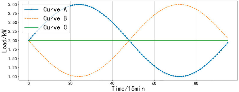
As shown in Figure 1, curves A and B are the daily load curves of residents A and B, respectively, and curve C is the cluster center of curves A and B. Among them, curve A reaches its peak in the first half of the curve. On the contrary, curve B reaches its peak in the second half of the curve. Curves A and B do not belong to the same type of residential load. However, the Euclidean distance between curve A, curve B, and cluster center C is respectively equal. If only Euclidean distance is used as the measurement standard for type classification, curves A and B will be classified into the same category. This is the isometry problem caused by Euclidean distance. Therefore, based on the above five types of daily load characteristic indicators, the maximum load occurrence time and minimum load occurrence time indicators are added to effectively distinguish the residential load curves in this paper. In summary, the clustering indicators of the daily load curves of residents selected in this chapter are shown in Table 1.

FIGURE 1

FIGURE 1. Three types of residential load curve.

TABLE 1

TABLE 1. Characteristic indicators based on daily load curve.

2.2 Clustering indicators of high-energy-consuming equipment

Air conditioners and electric water heaters are two types of high-power household adjustable loads. Based on these two types of electricity load curves, the analysis of clustering indicators is important for optimizing the clustering results of residential electricity consumption patterns. The relevant power consumption characteristics of high-energy-consuming equipment preliminarily selected are shown in Table 2. Among them, considering that the air conditioning load and the electric water heater load are both temperature-sensitive loads (Nanda et al., 2011), this paper refers to (Huang et al., 2012), and sets three indicators of daily load rate, weekly imbalance rate, and quarterly load rate, respectively, which intuitively reflects the short-term and long-term load volatility of these two types of loads. The price elasticity of average air-conditioning electricity demand during valley-to-peak hours and the price elasticity of average air-conditioning electricity demand during peak-to-valley reflect the enthusiasm of residents to participate in demand response projects under the premise of the implementation of the time-of-use electricity price policy. The specific definition and physical significance of relevant indicators are shown in Table 2.

TABLE 2

TABLE 2. Preliminary set of power consumption characteristics of high-energy-consuming equipment.

2.3 Selection of clustering indicators

Among the indicators selected in Section 2.1, the daily load characteristic indicator is a common setting in the current clustering research, while there are two problems in the clustering indicators of the power consumption characteristics of high-energy-equipment. On the one hand, the indicators do not necessarily collect enough information. On the other hand, the current indicator dimension is too high, resulting in redundant data information. Given the above problems, this section will calculate the contribution rate of each load power consumption characteristic indicator by principal component analysis (PCA) method, determine the first several indicators whose cumulative contribution rate reaches 90% as main components, and complete the elimination of redundant indicators while selecting indicators with complete information.

The variance interpretation rate is used to calculate the weight of each component based on the principle of information concentration of the data by PCA (Nie et al., 2009). The specific implementation steps of the PCA algorithm are as follows.

1) Based on the air conditioning load and electric water heater load data of 600 residents in a certain community, 20 refined load electricity characteristic indicators for each resident are calculated, forming a matrix of residential load characteristics indicators with a number of 600 × 20 rows:-

$X=\left(x_{n,j}\right)=\left[\begin{array}{cccc}{x}_{\mathrm{1,1}}& x_{\mathrm{1,2}}& \cdots & x_{\mathrm{1,20}}\\ x_{\mathrm{2,1}}& x_{\mathrm{2,2}}& \cdots & x_{\mathrm{2,20}}\\ ⋮& ⋮& \ddots & ⋮\\ x_{\mathrm{600,1}}& x_{\mathrm{600,2}}& \cdots & x_{\mathrm{600,20}}\end{array}\right],n=\mathrm{1,2},\dots ,600,j=\mathrm{1,2},\dots ,20(1)$

2) Calculate the correlation coefficient matrix of the clustering characteristic index factors $R={\left[R_1,R_2,\cdots ,R_{20}\right]}^T$;

3) Solve the eigenvalues of eigenequation ${\lambda }_1\ge {\lambda }_2\ge \cdots \ge {\lambda }_{20}\ge 0$ (arranged from the largest to the smallest), and calculate the eigenvectors $a_j\left(j=\mathrm{1,2},\cdots ,20\right)$ corresponding to each eigenvalue ${\lambda }_j$. Then, the original characteristic variable $X_1,X_2,\cdots ,X_{20}$ can be updated to $Z=\alpha X$ by linear transformation where $Z$ is the new feature variable after feature dimensionality reduction, that is, the extracted principal components $m$;

4) The contribution rate of the principal component $i$ and the cumulative contribution rate of the top components $m$ are calculated separately.

Cattell Lithotripsy is used to determine the principal indicator number. The contribution rate of each indicator is shown in Figure 2.

FIGURE 2

FIGURE 2. Gravel distribution map.

The corresponding indicators of the top five contribution rates are daily load rate of air conditioning, daily load rate of electric water heater, price elasticity of electric water heater electricity demand in valley-to-peak, price elasticity of air conditioning electricity demand in valley-to-peak, and the price elasticity of air conditioning electricity demand in peak-to-valley. The contribution degrees are: [.321, .258, .218, .140, and .043] and the cumulative contribution rate is as high as .980, which can ensure that the selected characteristic indicators can reflect the complete information.

3 Electricity consumption pattern clustering based on combined weighting

3.1 Weighting of clustering indicator based on the combination of entropy method and CRITIC method

In most of the studies, the entropy method is used to calculate the weight of the selected principal components, which provides an objective basis for the comprehensive analysis of multiple indicators and enhances the rigor of analysis. The entropy method is an enabling method based on the principle of entropy value in physics (Han et al., 2020). The smaller difference between different objects of the same indicator means a smaller amount of information and a greater entropy value. The entropy value of a certain characteristic indicator determines the size of its weight. The specific calculation steps of the entropy method are as follows.

1) Identify the negative elements in the characteristic indicator matrix $X=\left(x_{i,j}\right)=\left[\begin{array}{cccc}{x}_{\mathrm{1,1}}& x_{\mathrm{1,2}}& \cdots & x_{\mathrm{1,12}}\\ x_{\mathrm{2,1}}& x_{\mathrm{2,2}}& \cdots & x_{\mathrm{2,12}}\\ ⋮& ⋮& \ddots & ⋮\\ x_{\mathrm{600,1}}& x_{\mathrm{600,2}}& \cdots & x_{\mathrm{600,12}}\end{array}\right]$ which is composed of 12 kinds of load electricity characteristic indicators. If there is a negative number, the matrix is re-normalized to a non-negative interval to obtain matrix $\mathbf{Y}$, and all elements are always non-negative in the subsequent probability calculation process. The standardization of each element is calculated as follows:

$y_{i,j}=\frac{x_{i,j}-\mathit{min}\left\{x_{1,j},x_{2,j},\cdots ,x_{n,j}\right\}}{\mathit{max}\left\{x_{1,j},x_{2,j},\cdots ,x_{n,j}\right\}-\mathit{min}\left\{x_{1,j},x_{2,j},\cdots ,x_{n,j}\right\}}(2)$

2) The proportion of the jth indicator of the ith analysis object is calculated according to the standardized non-negative matrix $\mathbf{Y}=\left(y_{i,j}\right)=\left[\begin{array}{cccc}{y}_{\mathrm{1,1}}& y_{\mathrm{1,2}}& \cdots & y_{\mathrm{1,12}}\\ y_{\mathrm{2,1}}& y_{\mathrm{2,2}}& \cdots & y_{\mathrm{2,12}}\\ ⋮& ⋮& \ddots & ⋮\\ y_{\mathrm{600,1}}& y_{\mathrm{600,2}}& \cdots & y_{\mathrm{600,12}}\end{array}\right]$ obtained in step 1) and the probability $p_{i,j}$ corresponding to each element in the matrix Y is:

$p_{i,j}=\frac{y_{i,j}}{{\displaystyle \sum }_{i=1}^n{y}_{i,j}}(3)$

Ensure that the sum of the probabilities of each indicator is one and $p_{i,j}$ forms the probability matrix P.

3) Calculate the information entropy and information utility value of each indicator according to the probability matrix P, and finally obtain the entropy weight of each indicator through normalization. The information entropy of indicator $j$ is:

$e_j=-\frac{1}{\mathit{ln}n}{{\displaystyle \sum }}_{i=1}^n{p}_{i,j}\mathit{ln}\left(p_{i,j}\right)\left(j=\mathrm{1,2},\cdots ,12\right)(4)$

where the purpose of dividing by $\ln n$ is to ensure that the entropy value of the information is always within the range [0, 1]. The greater the information entropy, the less information indicator $\mathbf{J}$ contains. According to the value of the information entropy (4), the information utility value of indicator $j$ is calculated. The size of the utility value is positively correlated with the size of the information corresponding to indicator $j$.

According to the above calculation steps, the 12 types of clustering indicators are normalized and weighted. The corresponding weight of each indicator is shown in Table 3.

TABLE 3

TABLE 3. Indicators weighted results based on entropy value method.

Different objective empowerment methods have different pros and cons due to their research principles. The CRITIC method is based on the correlation of indicators, and its performance is better than the entropy method for indicators with strong volatility. The calculation principle of the CRITIC method is based on two aspects: The degree of difference between indicators and the degree of positive correlation between indicators. The former uses standard deviation for characterization, the larger the standard deviation, the greater the fluctuation, the more sufficient the amount of information, and the greater the weight. The latter is expressed by the correlation coefficient, the larger the value of the correlation coefficient, the less conflict between indicators and the smaller the weight. The specific calculation steps of the CRITIC weight method are (Xu et al., 2020).

1) By calculating the standard deviation of different indicator vectors to measure the difference and volatility of different indicators, the standard deviation calculation formula of the jth indicator is:

$S_j=\sqrt{\frac{{\displaystyle \sum }_{i=1}^n{\left(x_{ij}-\frac{1}{n}{\displaystyle \sum }_{i=1}^n{x}_{ij}\right)}^2}{n-1}}(5)$

where $x_{ij}$ is the jth indicator value of the ith resident and $\frac{1}{n}{\displaystyle \sum }_{i=1}^n{x}_{ij}$ is the average value of the jth indicator. The number of indicators $j=1,2,...,12,$ and the total number of households with a load n = 600.

2) Use the correlation coefficient of the jth indicator to measure the degree of positive correlation between indicators:

$R_j={{\displaystyle \sum }}_{i=1}^m\left(1-r_{ij}\right)(6)$

where $m=12$ is the correlation coefficient between indicator $i$ and indicator $j$. If the correlation between an indicator and other indicators is strong, it means that the data redundancy of the indicator is high and the amount of duplicate information is large, and the evaluation role of the indicator in clustering should be weakened, that is, its weight size should be reduced.

3) Calculate the amount of information $C_j$ and weight of the $j$-th indicator $W_j$:

$C_j=S_j\times R_j(7)$

$W_j=\frac{C_j}{{\displaystyle \sum }_{i=1}^m{C}_j}(8)$

Comparing the principles of entropy method and CRITIC method, it can be found that compared with the entropy method, the CRITIC method pays more attention to the original properties of the indicator, so the combination of the two empowerment methods can give full play to the advantages of the two. The CRITIC algorithm is weighted for 12 types of load characteristic indicators, and the results are shown in Table 4.

TABLE 4

TABLE 4. Indicators weighted results based on CRITIC method.

Compared with the weight values based on the entropy method in Table 3, the weight distribution calculated based on the CRITIC method is very different. In Table 3, the first three indicators with the largest weight are the daily load rate, the highest utilization hour rate, and the minimum load occurrence time, which are all indicators extracted based on the daily load characteristics. According to the principle of CRITIC algorithm, the daily load of residents has strong volatility, and the characteristic indicators extracted based on daily load themselves have strong randomness and conflict. Therefore, the daily load characteristic indicator will obtain a greater CRITIC weight than the refined load power consumption characteristic indicator. Then, multiply the entropy weight of each indicator shown in Table 3 with the CRITIC weight shown in Table 4 one by one and do normalization, and obtain the composite weight calculated according to the above steps to obtain the final weight of all indicators as shown in Table 5.

TABLE 5

TABLE 5. Final indicators weighted results.

3.2 Electricity consumption pattern clustering based on weighted clustering indicators

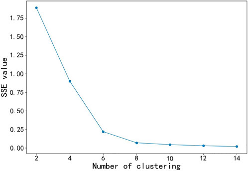
The weighted clustering indicator matrix is used as the input of the K-means algorithm to complete the clustering study of the electricity consumption patterns of all residential load. However, the cluster number $K$ of the K-means algorithm needs to be set in advance, and this chapter uses the elbow method and the contour coefficient method to jointly determine the optimal number of clusters. The basic principle of the elbow method is that as the number of divided categories increases, the sum of the squared errors (SSE) of each element in each category will continue to decrease, and the decline will decrease sharply; When a certain inflection point is reached, the polyline will flatten as the $K$ value continues to increase, and the corresponding value of that inflection point is selected as the final cluster number. The calculation formula of SSE is:

$SSE={{{\displaystyle \sum }}_{i=1}^k{{\displaystyle \sum }}_{Y_j\in S_k}\left|Y_j-C_i\right|}^2(9)$

where SSE represents the clustering error of all samples and reflects the clustering effect. When the total number of selected clusters $K$ is less than the actual number of clusters, increasing the set $K$ value can significantly improve the degree of intra-cluster aggregation of each cluster, which is manifested as a large decrease in SSE. When $K$ gradually increases to close to the true number of clusters, the improvement of the clustering effect is no longer obvious, and the trend of the SSE curve will also flatten.

The contour coefficient for a sample is calculated as follows:

$S\left(j\right)=\frac{b\left(i\right)-a\left(i\right)}{\mathit{max}\left\{a\left(i\right),b\left(i\right)\right\}}(10)$

where $a\left(i\right)$ represents the difference between samples in each category cluster; $b\left(i\right)$ represents the difference between samples in different categories of clusters. The average value of the contour coefficient of all samples is the contour coefficient of the clustering result, and its value is between [−1, 1], the larger the value means the higher the similarity of the samples divided in the category, the lower similarity of the samples between different classes, and the better clustering effect.

In order to select effective evaluation indicators to judge the clustering effect of improved clustering methods, this chapter introduces S_Dbw evaluation indicators based on literature (Naware et al., 2022). S_Dbw is an indicator for evaluating cluster quality based on the sum of the average intra-cluster compactness and inter-cluster density (ID) of each cluster. Smaller values for the evaluation metric mean better clustering.

4 Residential load forecasting based on residential electricity consumption pattern clustering and fully connected deep neural network

Since the key influencing factors of the electricity consumption characteristics of each residential load may have a non-linear relationship with the residential load, deep learning training modeling for the combination of variables with a non-linear relationship can obtain a load forecasting model with stronger generalization ability (Wang et al., 2020a; Wang et al., 2020b; Ismail et al., 2020). As a branch of machine learning, deep learning has been widely used since its proposal in 2006, which upgrades traditional neural network models (Cao et al., 2019; Kong et al., 2017a), has strong learning ability and adaptability, often used to solve many complex problems (Wang et al., 2019; Lu et al., 2019). Based on the basic principle of backpropagation, the fully connected deep neural network uses the gradient descent method to reduce the value of the loss function calculated in the process of forward propagation data, to complete the adaptive optimal parameter update.

The “full connection” of FDNN is reflected in the fact that all nodes in each layer will be connected to all nodes in the next layer, that is, there is a one-to-one correspondence mathematical relationship. “Depth” is reflected in the high number of layers in the model, which is usually set with multiple hidden layers. A neural network with a reasonable “depth” may fit better for model inputs with a larger amount of data (Lu et al., 2019; Qian et al., 2019; Wang et al., 2021). Considering that the neural network has too many hidden layers, it also leads to the overfitting of model training and the decrease of training rate, especially for the short-term load prediction problem (Hu et al., 2018; Dubey et al., 2021). Therefore, the FDNN model in this paper chooses to use a single-layer hidden layer, which can also obtain better generalization ability.

As mentioned above, the FDNN multi-task load forecasting model aims to minimize the loss function generated by forward propagation, and iteratively optimizes the parameters and b of each layer of the model. Considering that the adaptive moment estimation (ADAM) learning algorithm has fast calculation speed and less memory occupation (Kingma et al., 2014), it can obtain a more efficient deep learning model, and this chapter uses the ADAM algorithm as the optimization method of model parameters to complete the parameter adjustment work. The parameter update formula of ADAM algorithm is as follows:

$\left\{\begin{array}{c}t\leftarrow t+1\\ g_t\leftarrow {\mathit{\nabla }}_{\theta }{f}_t\left({\theta }_{t-1}\right)\\ m_t\leftarrow {\beta }_1\cdot m_{t-1}+\left(1-{\beta }_1\right)\cdot g_t\\ v_t\leftarrow {\beta }_2\cdot v_{t-1}+\left(1-{\beta }_2\right)\cdot g_t^2\\ m_t\sim \leftarrow m_t/\left(1-{{\beta }_1}^t\right)\\ \stackrel{\sim }{v_t}\leftarrow v_t/\left(1-{{\beta }_2}^t\right)\\ {\theta }_t\leftarrow {\theta }_{t-1}-a\cdot {\stackrel{\sim }{m}}_t/\left(\sqrt{\stackrel{\sim }{v_t}}+\epsilon \right)\end{array}\right.(11)$

where the left side of $\leftarrow$ is the output result, and the right side is the input result ${\theta }_t$ represents the parameters of the network; $g_t$ represents the gradient; $m_t$ and $m_t\sim$ represent the first-order moment estimates of the gradient $g_t$ before and after correction, respectively. $v_t$ and $\stackrel{\sim }{v_t}$ represent the second-order moment estimates of the gradient before and after correction, respectively. The default settings for the remaining parameters are: $a=0.001$, ${\beta }_1=0.9$, ${\beta }_2=0.999$, $\epsilon =10^{-8}$. It can be seen that the Adam algorithm calculates the adaptive learning rate of different parameters by calculating the mean of the first and second order moments of the gradient, making the update process of each parameter more independent (11). In addition, this chapter selects the Rectified Linear Unit (ReLU) function as the activation function of FDNN to further increase the model non-linearity. Compared with other types of activation functions, the advantage of the ReLU function is that it can effectively overcome the problem of vanishing gradients and speed up model training.

In order to improve the prediction effect of the FDNN model, all input data of the model should be standardized, and the convergence speed of the normalized neural network will be greater than that of the unstandardized (Cui et al., 2015). In this paper, the min-max standardization method is used to make linear changes to the original input data:

$x^{*}=\frac{x-\mathit{min}}{\mathit{max}-\mathit{min}}(12)$

where min and max represent the minimum and maximum values of the sample feature set, respectively.

5 Simulation results

5.1 Experiment setup

According to the SSE line chart shown in Figure 3 and the calculation result of the contour coefficient, K = 6 is selected as the number of clusters of the K-means algorithm in this paper, when the contour coefficient is the largest, and its value was .649.

FIGURE 3

FIGURE 3. SSE line chart.

In load forecasting, in addition to considering the temperature factor, the historical data of air conditioning load is also used as the input of the forecasting model. According to the data of a community in Jiangsu Province from 1 June 2019, to 31 May 2020, the residential load forecasting method proposed in this paper is used for different research. The specific settings are as follows:

Training set: 1 June 2018 to 31 May 2019.

Verification set: Summer (1 June 2019 to 31 July 2019), Autumn (1 September 2019 to 31 October 2019), Winter (1 December 2019 to 31 January 2020), Spring (1 March 2020 to 30 April 2020).

Test Set: Summer (1 August 2019 to 31 August 2019), autumn (1 November 2019 to 30 November 2019), Winter (1 February 2019 to 29 February 2020), Spring (1 May 2020 to 31 May 2020).

This paper forecasts load on a certain day in June and simulates it on a computer with Intel Core i5 1.4 GHz CPU and 8 GB memory.

5.2 Comparison of the clustering effect

Considering the volatility and diversity of resident load data, the following methods are set as the comparison methods of the improved clustering algorithm proposed in this chapter.

1) Direct K-means clustering of 96-dimensional daily load data;

2) The 96-dimensional data of the daily load curve of residents were weighted by the CRITIC algorithm and clustered by K-means;

3) Only the entropy method is used to weight the 12 types of clustering indicators, and then K-means is used for clustering;

4) K-means clustering based on 12 types of unweighted clustering indicators;

5) The entropy method and the CRITIC method are used to combine and weigh the seven types of daily load characteristic indicators, and then K-means are used for clustering.

The clustering result of the above five methods and the methods proposed in this chapter is evaluated using S_Dbw evaluation indicators. As shown in Table 6, the clustering results obtained by the proposed method correspond to the smallest value of the S_Dbw indicator, which proves that when selecting and analyzing the clustering indicator, considering the relevant indicators of refined load power consumption characteristics is also beneficial to improve the robustness of the clustering algorithm.

TABLE 6

TABLE 6. Assessment of cluster results.

5.3 Analysis of the result

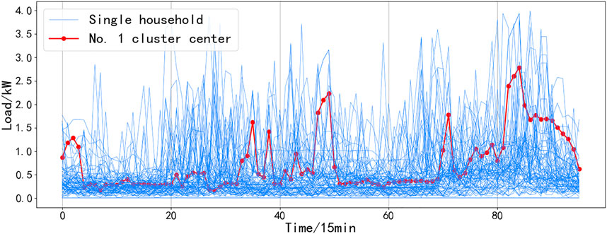
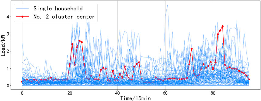
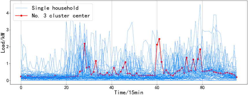
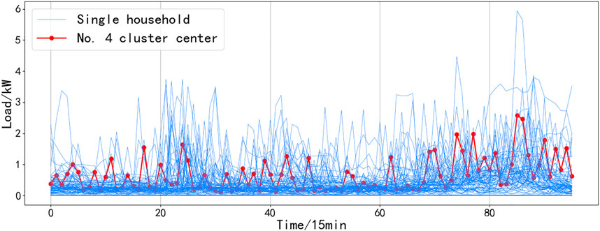
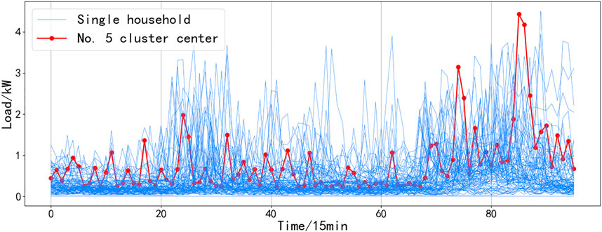
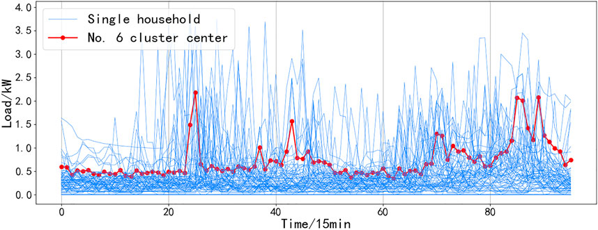
A load of residents in a certain community is clustered, and the results are shown in Figures 4–9. It can be seen from the figure that even if all resident samples belong to the same community, the living conditions and economic conditions are roughly the same, and there will be obvious differences between different residential load curves. Combined with Figures 4–9, the curve morphological characteristics of various residential cluster centers were analyzed, and different types of residents were qualitatively described. Category 1 residents still consume electricity above the average daily load during the period from 10:00 p.m. to 1:00 a.m. and belong to night owl families. The load curves of Category 2 and Category 6 residents have obvious morning, middle, and evening peaks, and the electricity consumption is low in other periods, which should be normal office worker families. The difference between the two is that the electricity consumption of Category 6 residents is low during lunch and dinner, and it can be inferred that their lunch and dinner are solved outside, while it can be seen from the load curve of Type 2 residents that the three meals of this type of residents are solved at home. The electricity consumption behavior of Category 3 residents is significantly weakened after 8:00 p.m., and the average electricity consumption of Category 3 residents is less than that of other categories, which should belong to elderly households or electricity-saving households. The load curve of Category 4 residents does not have very significant peak-to-valley characteristics, and the frequency of electricity consumption is high, which should belong to freelance families. Category 5 residents are other households.

FIGURE 4

FIGURE 4. Category 1 of residential electricity mode and the clustering center of it.

FIGURE 5

FIGURE 5. Category 1 of residential electricity mode and the clustering center of it.

FIGURE 6

FIGURE 6. Category 1 of residential electricity mode and the clustering center of it.

FIGURE 7

FIGURE 7. Category 1 of residential electricity mode and the clustering center of it.

FIGURE 8

FIGURE 8. Category 1 of residential electricity mode and the clustering center of it.

FIGURE 9

FIGURE 9. Category 1 of residential electricity mode and the clustering center of it.

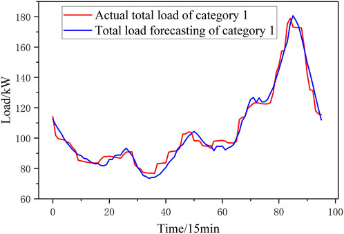
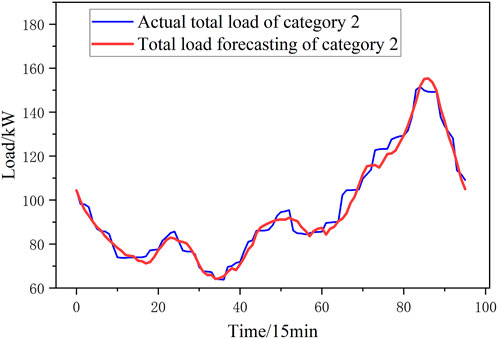
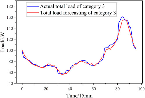
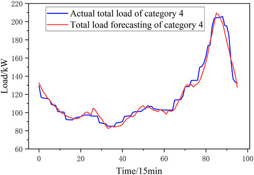
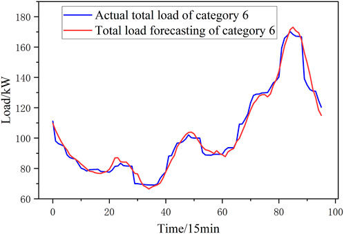
In this paper, a 1-day load of the summer is taken as an example, and the prediction results are shown in Figures 10–15. This paper uses the Mean Absolute Percentage Error (MAPE) to evaluate the accuracy of the prediction. The MAPE values for the six categories of loads forecast in this paper are [3.21%, 2.84%, 3.17%, 3.15%, 3.15%, 2.65%, and 2.87%]. Compared with the MAPE values for total load forecast without clustering, the MAPE value in this paper is 2.44%, 5.21% lower, which is shown in Figure 16. Prediction accuracy under different clustering methods is similar with prediction accuracy without different clustering methods, which shows that poor clustering methods cannot improve the accuracy of predictions.

FIGURE 10

FIGURE 10. Forecasting result of Category 1.

FIGURE 11

FIGURE 11. Forecasting result of Category 2.

FIGURE 12

FIGURE 12. Forecasting result of Category 3.

FIGURE 13

FIGURE 13. Forecasting result of Category 4.

FIGURE 14

FIGURE 14. Forecasting result of Category 5.

FIGURE 15

FIGURE 15. Forecasting result of Category 6.

FIGURE 16

FIGURE 16. Comparison of total load between mothod in this paper and forecasting without clustering.

6 Conclusion

This paper studies the problem of resident load forecasting and extracts seven commonly used daily load clustering indicators based on the daily load curve. At the same time, 20 types of clustering indicators are extracted based on the characteristics of the air conditioning load and electric water heater load. In order to avoid the overfitting problem caused by excessive indicator dimensions, the PCA method is used to process the characteristic indicators of high energy consumption, and 12 types of residential load clustering indicators are determined. To reduce the influence of subjectivity in indicator setting on the clustering results, the objective weighting method is used to empower 12 types of clustering indicators, and the K-means clustering of residential electricity consumption mode is completed based on the weighted indicator matrix. Among them, to give full play to the advantages of different objective weighting methods, the entropy method, which reflects the degree of dispersion between indicators, is combined with the CRITIC method, which comprehensively reflects the correlation within the indicator and the conflict between indicators, to obtain the weight calculation results with a higher degree of objectivity.

The results show that the proposed method can obtain the clustering results with the smallest S_Dbw value, and the clustering effect is the best. Finally, multi-task learning is carried out based on the load historical data of different types of residents, and the load prediction results of six types of residents are obtained through FDNN. The comparison shows that the accuracy of the prediction method proposed in this paper is improved.

With the development of science and technology, the structure of the power grid will be more complex than before, and the balance between supply and demand of power load will also face new challenges. The load forecasting model built in this paper has good forecasting performance, but there are still some problems to be studied and improved.

1) Because new energy power generation is affected by many factors, such as light, wind speed, wind direction, etc., the relationship between short-term power load and influencing factors may also change, and new hidden influencing factors and related relationships need to be explored.

2) The data used in this paper are partly from 2019. Affected by COVID-19 in 2020, the global economic pattern and energy consumption structure have been greatly affected, which also poses new challenges to load forecasting.

Data availability statement

The raw data supporting the conclusion of this article will be made available by the authors, without undue reservation.

Author contributions

KY, JC, and ZY contributed to the conception and design of the study. KY organized the database. XC and LG performed the statistical analysis. ZY wrote the first draft of the manuscript. JC wrote sections of the manuscript. All authors contributed to manuscript revision, read, and approved the submitted version.

Funding

This research is supported by Jiangsu Provincial Key R&D Program “Research and Engineering Demonstration of Key Technologies for Low Carbon Future Buildings” (Project No. BE2022606).

Conflict of interest

The authors declare that the research was conducted in the absence of any commercial or financial relationships that could be construed as a potential conflict of interest.

Publisher’s note

All claims expressed in this article are solely those of the authors and do not necessarily represent those of their affiliated organizations, or those of the publisher, the editors and the reviewers. Any product that may be evaluated in this article, or claim that may be made by its manufacturer, is not guaranteed or endorsed by the publisher.

References

Cannas, B., Carcangiu, S., Carta, D., Fanni, A., and Muscas, C. (2021). Selection of features based on electric power quantities for non-intrusive load monitoring. Appl. Sci. 11 (2), 533. doi:10.3390/app11020533

CrossRef Full Text | Google Scholar

Cao, Z., Wan, C., Zhang, Z., Li, F., and Song, Y. (2019). Hybrid ensemble deep learning for deterministic and probabilistic low-voltage load forecasting. IEEE Trans. Power Syst. 35 (3), 1881–1897. doi:10.1109/tpwrs.2019.2946701

CrossRef Full Text | Google Scholar

Cui, M., Zhang, J., Florita, A. R., Hodge, B. M., Ke, D., and Sun, Y. (2015). An optimized swinging door algorithm for identifying wind ramping events. IEEE Trans. Sustain. Energy 7 (1), 150–162. doi:10.1109/tste.2015.2477244

CrossRef Full Text | Google Scholar

Du, S., Li, M., Han, S., Shi, J., and Li, H. (2019). Multi-pattern data mining and recognition of primary electric appliances from single non-intrusive load monitoring data. Energies 12 (6), 992. doi:10.3390/en12060992

CrossRef Full Text | Google Scholar

Dubey, S. R., and Chakraborty, S. (2021). Average biased ReLU based CNN descriptor for improved face retrieval. Multimedia Tools Appl. 80 (15), 23181–23206. doi:10.1007/s11042-020-10269-x

CrossRef Full Text | Google Scholar

Fujimoto, Y., Fujita, M., and Hayashi, Y. (2021). Deep reservoir architecture for short-term residential load forecasting: An online learning scheme for edge computing. Appl. Energy 298, 117176. doi:10.1016/j.apenergy.2021.117176

CrossRef Full Text | Google Scholar

Han, F., Pu, T., Li, M., and Taylor, G. (2020). Short-term forecasting of individual residential load based on deep learning and K-means clustering. CSEE J. Power Energy Syst. 7 (2), 261–269.

Google Scholar

Hong, Y., Zhou, Y., Li, Q., Xu, W., and Zheng, X. (2020). A deep learning method for short-term residential load forecasting in smart grid. IEEE Access 8, 55785–55797. doi:10.1109/access.2020.2981817

CrossRef Full Text | Google Scholar

Hou, T., Fang, R., Tang, J., Ge, G., Yang, D., Liu, J., et al. (2021). A novel short-term residential electric load forecasting method based on adaptive load aggregation and deep learning algorithms. Energies 14 (22), 7820. doi:10.3390/en14227820

CrossRef Full Text | Google Scholar

Hu, Z., Li, Y., and Yang, Z. (2018). “Improving convolutional neural network using pseudo derivative ReLU,” in Proceedings of the 2018 5th International Conference on Systems and Informatics (ICSAI), Nanjing, China, November 2018 (IEEE), 283–287.

CrossRef Full Text | Google Scholar

Hua, H., Qin, Y., Hao, C., and Cao, J. (2018). Stochastic optimal control for energy internet: A bottom-up energy management approach. IEEE Trans. Industrial Inf. 15 (3), 1788–1797. doi:10.1109/tii.2018.2867373

CrossRef Full Text | Google Scholar

Huang, G., Wang, M., and Wang, G. (2012). Research on empowerment by improved entropy method in performance evaluation. Comput. Eng. Appl. 48 (28), 245–248.

Google Scholar

Ismail, M., Shaaban, M. F., Naidu, M., and Serpedin, E. (2020). Deep learning detection of electricity theft cyber-attacks in renewable distributed generation. IEEE Trans. Smart Grid 11 (4), 3428–3437. doi:10.1109/tsg.2020.2973681

CrossRef Full Text | Google Scholar

Kingma, D. P., and Ba, J. (2014). Adam: A method for stochastic optimization. https://arxiv.org/abs/1412.6980.

Google Scholar

Kong, W., Dong, Z. Y., Jia, Y., Hill, D. J., Xu, Y., and Zhang, Y. (2017). Short-term residential load forecasting based on LSTM recurrent neural network. IEEE Trans. Smart Grid 10 (1), 841–851. doi:10.1109/tsg.2017.2753802

CrossRef Full Text | Google Scholar

Lee, E., and Rhee, W. (2021). Individualized short-term electric load forecasting with deep neural network-based transfer learning and meta learning. IEEE Access 9, 15413–15425. doi:10.1109/access.2021.3053317

CrossRef Full Text | Google Scholar

Lin, W., Wu, D., and Boulet, B. (2021). Spatial-temporal residential short-term load forecasting via graph neural networks. IEEE Trans. Smart Grid 12 (6), 5373–5384. doi:10.1109/tsg.2021.3093515

CrossRef Full Text | Google Scholar

Liu, D., Qin, Z., Hua, H., Ding, Y., and Cao, J. (2023). Incremental incentive mechanism design for diversified consumers in demand response. Appl. Energy 329, 120240. doi:10.1016/j.apenergy.2022.120240

CrossRef Full Text | Google Scholar

Lu, J., Zhang, Q., Yang, Z., Tu, M., Lu, J., and Peng, H. (2019). Short-term load forecasting method based on CNN-LSTM hybrid neural network model. Automation Electr. Power Syst. 43 (8), 131–137.

Google Scholar

Lusis, P., Khalilpour, K. R., Andrew, L., and Liebman, A. (2017). Short-term residential load forecasting: Impact of calendar effects and forecast granularity. Appl. energy 205, 654–669. doi:10.1016/j.apenergy.2017.07.114

CrossRef Full Text | Google Scholar

Nanda, A., and Pujari, A. K. (2011). “Weighted co-clustering based clustering ensemble,” in Proceedings of the 2011 Third National Conference on Computer Vision, Pattern Recognition, Image Processing and Graphics, Hubli, India, December 2011 (IEEE), 46–49.

CrossRef Full Text | Google Scholar

Naware, D., and Mitra, A. (2022). Weather classification-based load and solar insolation forecasting for residential applications with LSTM neural networks. Electr. Eng. 104 (1), 347–361. doi:10.1007/s00202-021-01395-2

CrossRef Full Text | Google Scholar

Nie, B., Du, J., Liu, H., Xu, G., Wang, Z., He, Y., et al. (2009). “Crowds’ classification using hierarchical cluster, rough sets, principal component analysis and its combination,” in Proceedings of the 2009 International Forum on Computer Science-Technology and Applications, Chongqing, China, December 2009 (IEEE), 287–290.1

Google Scholar

Piao, M., Shon, H. S., Lee, J. Y., and Ryu, K. H. (2014). Subspace projection method based clustering analysis in load profiling. IEEE Trans. Power Syst. 29 (6), 2628–2635. doi:10.1109/tpwrs.2014.2309697

CrossRef Full Text | Google Scholar

Qian, K., Shen, J., and Liu, Y. (2019). Accurate score incentive mechanism of resident demand response based on load clustering. Power Econ. 47 (7), 29–35.

Google Scholar

Rodriguez, A., and Laio, A. (2014). Clustering by fast search and find of density peaks. science 344 (6191), 1492–1496. doi:10.1126/science.1242072

PubMed Abstract | CrossRef Full Text | Google Scholar

Wang, B., Li, Y., Ming, W., and Wang, S. (2020b). Deep reinforcement learning method for demand response management of interruptible load. IEEE Trans. Smart Grid 11 (4), 3146–3155. doi:10.1109/tsg.2020.2967430

CrossRef Full Text | Google Scholar

Wang, L., Zhou, Q., and Jin, S. (2020a). Physics-guided deep learning for power system state estimation. J. Mod. Power Syst. Clean Energy 8 (4), 607–615. doi:10.35833/mpce.2019.000565

CrossRef Full Text | Google Scholar

Wang, S., Deng, X., Chen, H., Shi, Q., and Xu, D. (2021). A bottom-up short-term residential load forecasting approach based on appliance characteristic analysis and multi-task learning. Electr. Power Syst. Res. 196, 107233. doi:10.1016/j.epsr.2021.107233

CrossRef Full Text | Google Scholar

Wang, Z., Zhao, B., Ji, W., Gao, X., and Li, X. (2019). Short-term load forecasting method based on GRU-NN model. Automation Electr. power Syst. 43 (5), 53–58.

Google Scholar

Xie, G., Chen, X., and Weng, Y. (2020). Input modeling and uncertainty quantification for improving volatile residential load forecasting. Energy 211, 119007. doi:10.1016/j.energy.2020.119007

CrossRef Full Text | Google Scholar

Xu, C., Ke, Y., Li, Y., Chu, H., and Wu, Y. (2020). Data-driven configuration optimization of an off-grid wind/PV/hydrogen system based on modified NSGA-II and CRITIC-TOPSIS. Energy Convers. Manag. 215, 112892. doi:10.1016/j.enconman.2020.112892

CrossRef Full Text | Google Scholar

Zhang, W., Hua, H., and Cao, J. (2017). “Short term load forecasting based on IGSA-ELM algorithm,” in Proceedings of the In2017 IEEE International Conference on Energy Internet (ICEI), Beijing, China, April 2017 (IEEE), 296–301.

CrossRef Full Text | Google Scholar

Zheng, Z., Chen, H., and Luo, X. (2019). A Kalman filter-based bottom-up approach for household short-term load forecast. Appl. Energy 250, 882–894. doi:10.1016/j.apenergy.2019.05.102

CrossRef Full Text | Google Scholar