Corrigendum: Particle Filter Based Range Search Approach for Localization of Radioactive Materials
 Imbaby I. Mahmoud
 Asmaa A. Abd el-Hamid
- Egyptian Atomic Energy Authority, Cairo, Egypt
Wireless Sensor Networks (WSNs) have recently become crucial in monitoring operations. The development of a Data Fusion Algorithm for radioactive source localization utilizing WSN based on the Particle Filter (PF) technique is presented. The localization of an unknown-intensity point radioactive source using sensor nodes measured intensities in Count per Minute (CPM) is considered. The surveillance area is covered by several sensors (radiation detectors) n. Instead of using four sensors, as described in previous research, two consecutive sensors are used in sequence (S1, S2), (S2, S3)……, (Sn-1, Sn) till reaching the last sensor available Sn. Apollonius circle calculated range guides a particle filter for estimating the source location using actual measurements. Compared with other approaches such as the Iterative Pruning Clustering algorithm, more accurate estimates in terms of the error between the estimated source position and ground truth are obtained. The comparison is conducted using the same real measurements data. The Particle Filter based algorithm is implemented in a Xilinx FPGA chip. The architecture is a two sequential steps implementation, where particle generation, weight calculation, and normalization are carried out in parallel during the first step, followed by a sequential or parallelized resampling in the second step. This architecture targets a balance between hardware resources and speed of operation. The future work plan includes security-related studies and complete WSN implementation using μC/FPGA devices.
1 Introduction
Motivating this work is the rush of Mid-east countries towards peaceful uses of atomic energy, impacting the national environmental situation. Since radioactive material monitoring becomes very important especially in the emerging nuclear regions, it is necessary to build instruments and systems to deal with radioactive material detection and tracking. Wireless Sensor Networks (WSNs) and μC/FPGA are proposed to implement these systems.
The problem of monitoring and searching for threats that involve radioactive materials is highly challenging because of the high variance in background radiation, the presence of non-harmful sources, and the possible shielding of harmful sources. We study in this paper a collection of algorithms and analyses that center around the problem of radiation detection with a distributed sensor network. Liu (2010) investigated the essential characteristics of a radiation sensor network focused on the tradeoffs between false positive rate, valid positive rate, and time to detect one or more radiation sources in a large area. She carried out mathematical and simulation evaluations of crucial system factors like sensor nodes and sensor position. Zhang (2012) proposed a statistical method based on the likelihood ratio test (conditional test statistic), accessed by the likelihood ratio statistic. Other researchers have addressed the problem of radiation source localization using different approaches. The geometric difference triangulation method is presented in (Wu et al., 2014) to estimate source location by solving a system of nonlinear equations for three measurement sensors. The Ratio of Square Distance (ROSD) method introduced in (Chin et al., 2010), presents a closed-form solution that can solve the imaginary root problem when dealing with more than 3 sensors. Various methods based on maximum likelihood estimation (MLE) (Gunatilaka et al., 2007) have been proposed. Henry E. Baidoo-Williams (Baidoo-Williams, 2016) used a non-concave maximum likelihood-based profit function to ensure a unique global maximizer. Cordone (2019) used linear regression (LR) to estimate the source and background intensities and then used these estimates to initialize the intensity parameter search for MLE.
Nageswara S. V. Rao et al. (Rao et al., 2008) proposed two localization methods: A mean of estimators (MoE) method and a mean of measurements (MoM) method that computed the mean of the measurements and showed from simulation results that MoE outperforms MoM. Chase Qishi Wu et al. (Wu et al., 2019) presented three localization-based detection approaches, namely: Source-attractor Radiation Detection (SRD), Triangulation-based Radiation Source Detection (TriRSD), and Ratio of Square Distance-based Radiation Source Detection (ROSD-RSD). Bayesian algorithms that compute an a posteriori probability distribution based on a given prior distribution and likelihood values calculated from measurements are illustrated in (Dalal and Han, 2010; Jarman et al., 2011; Liu et al., 2011; Rao et al., 2015; Tandon et al., 2016). Mobile sensor networks, which study real-time challenges for moving sources are studied (Rao et al., 2015). N. Rao et al. (Rao et al., 2015) suggested a Particle Filter algorithm, where it has been used in a border monitoring scenario. A geostatistical interpolation method that uses the given measurements to estimate positions where data were not collected based on Poisson kriging is presented (Zhao et al., 2019). Fragkos et al. (2020) developed a fusion algorithm based on an analytical procedure for five sensors. This analytical method did not consider the geometrical form factors of the sensors and the radiation attenuation of the medium between the source and the sensors, which contributed to lower localization accuracy. The localization algorithms, which are based on machine learning techniques, such as Artificial Neural Networks (ANN) and Boosted Decision Trees (BDT) are also investigated (Kyriakis and Karafasoulis, 2020). J.-C. Y. Chin et al. (Chin et al., 2008) claimed an accurate localization method under noise and measurement errors.
This paper develops a robust data fusion and parameter estimation method for radioactive source localization based on the Particle Filter algorithm. The presented Particle Filter based algorithm is implemented in a Xilinx FPGA chip. Sensor nodes, as well as base stations, can be implemented using μC/FPGA chips. The proposed approach is evaluated and compared with other techniques reported in (Chin et al., 2008).
This paper is organized as follows. In Section 2, a brief review of the most common fusion-based localization approaches is presented. Then, Section 3 demonstrates the proposed algorithm and its flow. Next, in Section 4, the experimental setup and the obtained results are discussed. Finally, an FPGA implementation of the proposed localization algorithm to speed up the localization process is presented in Section 5, followed by the conclusion.
2 Review of Approaches for Radioactive Source Localization
In (Chin et al., 2010; Liu, 2010), a summary, classification, and drawbacks of methods used for localization problems are reported. The following summarizes previous work in fusion of data collected from sensor network approaches for radioactive source localization.
2.1 Data Fusion From Multiple Sensors
Data collected at more than one sensor can be combined or considered separately. The former is often referred to as the “data fusion” step. Algorithms without data fusion make decisions based on readings from a single detector only and thus require no sensor-to-sensor or sensor-to-server communication. On the other hand, algorithms that fuse sensor data require the data to be transferred to one or a few centralized servers (base stations) for processing, creating more complexity in system architecture and introducing higher costs. Therefore, it is essential to understand and quantify the benefits of sensor data fusion when designing a radiation sensor network. For example, if the independent analysis is almost as good as algorithms with data fusion, communication between sensors can be simplified.
Data fusion is undoubtedly advantageous for discovering and recognizing a source, but it is unclear how much if at all, it improves detection. While simply integrating data (e.g., summing all data without filtering) improves signal strength, it also introduces noise, lowering SNR. The combined SNR may be lower than considering SNR from each sensor individually. For example, view a grid of widely-spaced sensors and a weak static source near one detector. The detector closest to the source will have a high SNR, whereas the other sensors receive mostly noise. Combining the data blindly from all four sensors will always decrease the overall SNR. More quantifying the benefits from data fusion can be found in (Chin et al., 2010; Liu, 2010).
2.2 Localization Approaches
In a noise- and error-free situation, determining the location of a radioactive source problem can be solved in closed form employing four ideal sensors and the Apollonius circle (Chin et al., 2008). When uncertainties and noise like background radiation are considered, more sensors are required to give correct results, especially for extremely low source intensities. In real-world scenarios, noise and measurement errors are unavoidable. Hence, the fusion of measurements from n sensors, n > 3, is necessary to increase the solution’s reliability.
2.2.1 Maximum Likelihood Estimator Method
The Maximum Likelihood Estimator (MLE) method constructs a maximum likelihood estimator and solves it with optimization techniques. It considers a uniform background whose strength has been measured as a priory, and the remaining unknown variables to be estimated are the source strength µ and source position X = (x, y). The discrete Poisson mass function is used as a radiation sensing model. MLE searches over a solution space of both the source strength and position, such that the difference between the predicted measurements according to the sensing model and the actual measurements by the n sensors is minimized. The method can converge on local minima, which leads to the detection of phantom sources.
2.2.2 Mean of Estimators Method
The mean of estimators (MoE) localization method (Rao et al., 2008) produces estimated results by linearly combining each subset of three sensors. The MoE method computes the fused estimate and the candidate estimates’ mean. The advantage of the MoE method is that it has linear time complexity and generally runs much faster than MLE. However, the fundamental flaw of MoE is that it isn’t specifically designed to eliminate phantom estimations during the fusion process. Phantom estimations can harm localization accuracy, especially if they appear to be generated by robust (and thus presumably accurate) sensor readings. As a result, when a significant portion of the candidate estimates is phantom estimates, this approach can provide substantial localization errors.
2.2.3 Iterative Pruning (ITP) Clustering Algorithm
The approach is divided into two parts, Clustering, and fusion (Chin et al., 2008). Clustering (Quality Threshold (QT) clustering) is used to find the smallest region in the surveillance area that contains a majority if not all, candidate estimates that are not phantom estimates. Fusion is used to compute a weighted centroid of the candidate estimates in the cluster found above as the fused estimate. After each iteration, the candidate estimates input into the technique are pruned iteratively until only the region with the most estimates remains. When the number of estimates left is less than N and the region’s area is less than d × d, the Algorithm stops. The N and d parameters limit the maximum number of estimates in the remaining region and the smallest region’s maximum size (in terms of area). The fused estimation is calculated from the weighted center of the remaining estimations. As the number of sensors increases, the candidate estimates increase as O (n3), where n is the number of sensors.
2.2.4 Bayesian Algorithms
Probabilistic representations account for uncertainty in the source location resulting from uncertainties in detector responses and the potential for non-unique solutions. A Bayesian approach improves previous likelihood methods for source localization by incorporating all available information to help constrain solutions. Bayesian algorithms generally give good results when the prior estimates of unknown parameters are accurate. However, they give wrong results when the preliminary estimates are poor and when the signal data is too small to overcome the poor prior forecast. A. Liu et al. (Liu et al., 2011) present a heuristic that combines classical parametric statistical algorithms (K-Sigma Algorithm) with Bayesian algorithms (Kalman filter) to deal with this problem. However, this heuristic could suffer from incorrect estimations from the parametric algorithm emphasized by the Bayes algorithm. Moreover, Bayes algorithm complexity increases exponentially with the number of sources.
2.2.5 AI Approach
G. Cordone (Cordone, 2019) presents a method to perform the MLE localization without prior knowledge of the background radiation intensity. It estimates the source and background intensities using linear regression (LR) and then uses these estimates to initialize the intensity parameter search for MLE. This method is tested using single-resolution, multi-resolution, and multi-resolution with grid expansion MLE algorithms, and performance is compared to MLE algorithms that don’t use the LR initialization. It is reported that using the LR estimates to initialize the intensity parameter search caused a marginal increase in both localization error and computation time for the tested algorithms. The technique is only beneficial in the case of unknown background intensity. The localization algorithms, which are based on machine learning techniques, such as Multi-Layer Perceptron Artificial Neural Networks (MLP) and Boosted Decision Trees (BDT) (Kyriakis and Karafasoulis, 2020), are also investigated. Using Cs-137 source of 180 micro-Curie (μCi), a localization accuracy of 15 and 10 cm in horizontal and vertical source coordinates respectively within an area of 5 m × 2.8 m covered by a sensor network consisting of five sensors has been achieved.
ALGORITHM 1

ALGORITHM 1. Algorithm Range Search PF Source Localizer.
3 Proposed Localization Approach
In this section, a data fusion method for radioactive source localization based on Particle Filter algorithm is developed. Apollonius circle calculated range of candidate source positions from every pair of two consecutive sensors of the n-sensor network is used to guide a Particle Filter for estimating the source location. The radius of the Apollonius circle is used in the particle filter likelihood function to converge to a source position estimate.
3.1 Problem Formulation
The localization of a point radiation source of unknown strength Au expressed in the unit of micro-Curie (μCi) called the source rate will be considered. The source is located at an unknown location (xu, yu). The source gives a radiation intensity of
(expressed in counts per minute or CPM) when measured by a sensor at point p = (x, y), where E is an efficiency constant unique to the sensor. The radiation count induced by the source and observed at the sensor i per unit time is a Poisson random variable with parameter λ = I(xi, yi), not accounting for the background radiation B(x, y) (Rao et al., 2008) denoting the background radiation strength at (x, y) expressed in CPM, called the background rate. The radiation count measurement (due to the background radiation) at a sensor i located at (xi, yi) is given by the Poisson random variable with parameter B(xi, yi). For comparison purposes, the radiation model, actual measurements, and calibration process (Rao et al., 2008) are followed.
3.2 Apollonius Circle
Apollonius Circle describes the locus of point p, which has a fixed distance from point A equal multiple of its distance from another fixed point B. If the m:n equals one, the locus is the perpendicular bisector of segment AB. If m ≠ n, then it is a circle (Kim, 2021).
In Figure 1, AP:BP = m:n. When the point P moves, keeping this ratio, the locus of p is a Circle, which is called the circle of Apollonius. This circle connects A and B’s interior and exterior division points (the interior bisector PP1 and the exterior bisector PP2 in Figure 2).
FIGURE 1
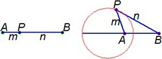
FIGURE 1. Apollonius circle.
FIGURE 2
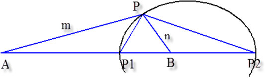
FIGURE 2. The interior bisector PP1 and the exterior bisector is PP2.
3.3 Particle Filter
Particle filter is a sequential Monte-Carlo approach used to estimate the dynamic state parameters of nonlinear and/or non-Gaussian systems (Fox et al., 1999; Marimon et al., 2007). The essential idea is to approximate the probability density functions (PDFs) of the state of a dynamic model by random samples (particles) with associated weights, then propagating them across iterations based on a probabilistic model of the state update and the measurements (Arulampalam et al., 2002).
J. Cook et al. (Cook et al., 2020) proved the theoretical convergence of the estimate to the state posterior probability density function of Particle Filter. So, weak convergence in radioactive source localization applications is not a problem.
A. Kyriakis and K. Karafasoulis (Kyriakis and Karafasoulis, 2020) pointed that Particle Filter algorithm complexity increases exponentially with the number of sources. Therefore, the next section of this paper presents a H/W implementation of the proposed Particle Filter to speed up the processing that can help deal with this situation and real-time scenarios.
3.4 Proposed Algorithm
The Particle Filter Range Search algorithm works as follows. Initially, the 1,000 particles are evenly distributed, i.e., the initial state of the source is entirely unknown. Then, it converges to a source position estimation after using the radius of the Apollonius circle in the particle filter likelihood function. Figure 3 illustrates the flow of the proposed Algorithm. First, two consecutive sensors (e.g., S1 and S2) readings are used to obtain a candidate position for the radioactive source. Next, two points (p1, p2) on an Apollonius circle are calculated. Then the radius of the circle r calculated according to Eq. 2 is used in the likelihood function of the particle filter. Finally, a probability is assigned to each particle according to the standard Gaussian formula, and their weights are calculated as in Eq. 3.
Where xs and ys are positions of the sensors in the environment.
Where rm is the range measurement (Apollonius)
FIGURE 3
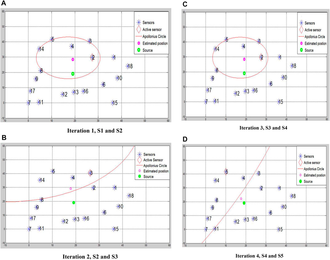
FIGURE 3. The flow of the Algorithm. (A) Iteration 1, S1 and S2 (B) Iteration 2, S2 and S3 (C) Iteration 3, S3 and S4 (D) Iteration 4, S4 and S5.
q = [x, y] is the state vector
r^ is the range estimate from the particle to the sensor
and σ: is the standard deviation from the PDF for that range measurement.
A pool of candidate particle positions is calculated, and an estimated source position is plotted as shown in Figure 3A. For the 2nd round, the next consecutive sensor (S3) reading with the previous sensor reading (S2) is used to form another Apollonius circle, as shown in Figure 3B. Finally, the particles are resampled from the previous round’s Apollonius circle perimeter particle pool. Figures 3C,D show the following rounds, which will continue till utilizing all 18 sensors.
The pseudo-code of the proposed algorithm can be stated as follows.
4 Results and Discussion of the Proposed Algorithm S/W Implementation
As we stated above, real measurements data from (Rao et al., 2008) is used to derive our experiment. The surveillance area is 50 × 50 cm, and the number of sensors distributed over this region is 18. The position of these sensors is shown in Table 1. A Cs-137 radiation point source emits Gamma-ray of intensity Au = 0.911 μCi and their position in the area (Xs,Ys) = (19.09,19.09). We consider that the distance measurements are in centimeters (cm). Matlab experimental setup for sensor and radiation source placements is depicted in Figure 4.
TABLE 1
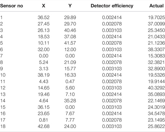
TABLE 1. Sensors Coordinates used in 0.911 μCi Cs-137 Source Experiments and Actual measurements.
FIGURE 4
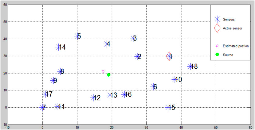
FIGURE 4. Matlab Experiment Setup (Sensor and radiation source placements).
Table 2 shows the error in estimated position values from one run of the proposed algorithm implemented Matlab program. Figure 5 shows that the error decreases when we observe readings from more sensors. However, it is not smooth monotonically reducing due to the random nature of the particle filter. Compared with ref. (Chin et al., 2008), superior results are achieved when the number of sensors is increased, as shown in Table 3 and Figure 6.
FIGURE 5
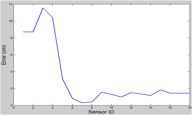
FIGURE 5. Error in Estimated Position values with the number of sensors.
TABLE 2
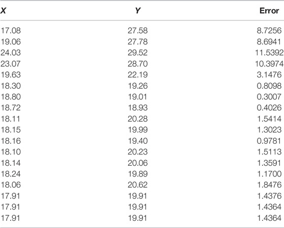
TABLE 2. Error of one run (not averaged).
TABLE 3
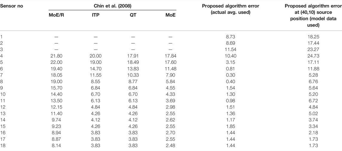
TABLE 3. Recorded error comparison between ref. (Chin et al., 2008). and the proposed Algorithm.
FIGURE 6
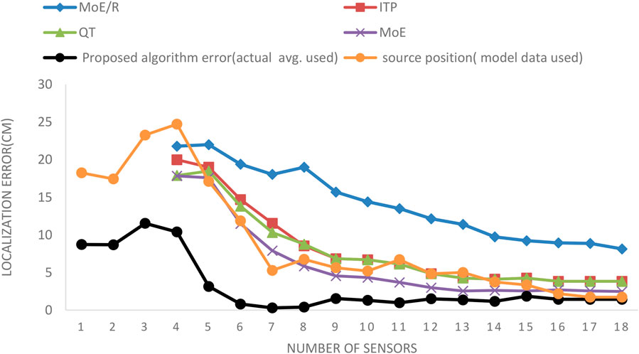
FIGURE 6. Comparison of Error in Estimated Position values related to the number of sensors between the proposed Algorithm and ref. (Chin et al., 2008). results.
Table 3 shows recorded error obtained from ref. (Chin et al., 2008). in the first column (four methods). The second column reports the values obtained from our Algorithm while using ref. (Chin et al., 2008). average of actual measured data and the last column represents values calculated using model data when the source is out of the area surrounded by the sensors [source is located at (40,10)]. The last case is unattained by all other approaches [RoSD (ratios of square distances) and log-space DTOA (time difference of arrival)] (Chin et al., 2008). Figure 6 depicts these results graphically.
The proposed algorithm outperforms the Iterative Pruning Clustering algorithm when using just four sensors and above. For sensor count less than four, the results of our Algorithm and reference three sensor treatment are comparable (not shown in the figure). From Figure 6, the Algorithm run with 6 sensors achieved the best tradeoff between the number of sensors and an estimated position error of 2%, 18 times less than the competitor (ITP) approach. Therefore, compared with other techniques, superior performance of the guided Particle Filter approach, in terms of localization error, is achieved. At the same time, adding 2 more sensors is not costly. Also, the proposed algorithm can localize a source, even when the area surrounded by the sensors does not contain that source.
Optimizing sensor placement can be implemented by maximizing a detection function F (Liu et al., 2011), defined as the sum of true positives over the whole area while keeping the false positive rate constant using a known source strength.
5 FPGA Implementation of Particle Filter Based Range Search Localization Algorithm
To speed up the proposed Algorithm, an FPGA implementation of particle filter based range search localization algorithm is introduced. Figure 7 shows the Sampling Importance Resampling Filter (SIRF). SIRF performs the particle generation and weight calculation for every input sample. After M particles pass, the weight normalization, outputting, and resample are carried out.
FIGURE 7
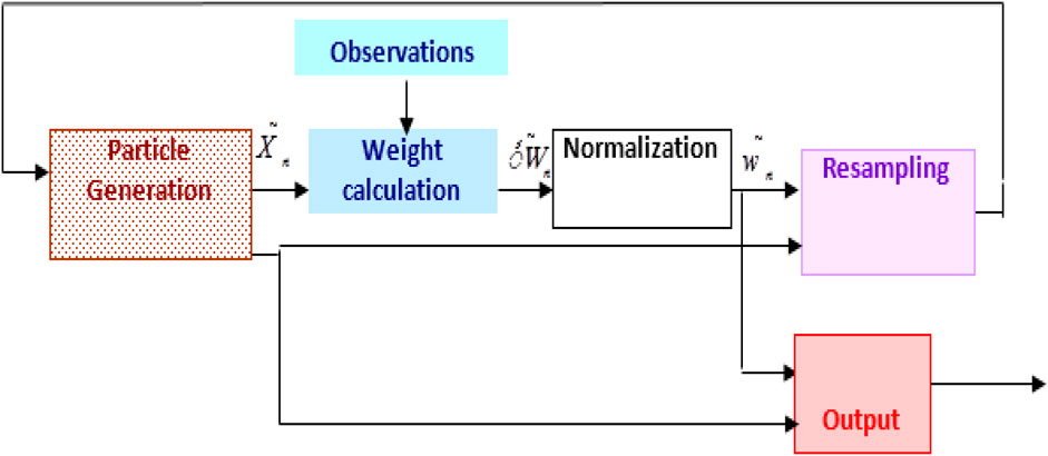
FIGURE 7. Sampling Importance resampling filter (SIRF).
5.1 Proposed Architecture
The proposed architecture, shown in Figure 8, uses 2MxP dual-port FIFO to store the particles, where M is the number of particles and p is a two-component state vector, given by (x, y) to represent the X-position and Y-position. Two registers files are used: The first Mxw register file stores the particle weights where w represents the length of weight bits. The second Mxn register file keeps the replication factor for each particle (M = 2n), where n is the replication number. Figure 8 illustrates the data flow through processing stages of the proposed radioactive source localization H/W architecture. The operations of this PF H/W architecture can be summarized as follows.
1) In sample engine, the particles are generated from samples drawn using the random number generator (Mahmoud et al., 2016). Then, in each moving step, all particles are drifted by the same amount. The generated particles are stored in a FIFO for routing when it has a replication value. As all particles are generated, they can be used for weight calculation.
2) In the weight calculation engine, initially, N particles are spread over the xy plane within the predetermined boundaries where the probability of each particle is (1/N). When the first particle rout is finished, the observation (rm) will be enabled and a probability is assigned to each generated particle according to a developed linearized function of the likelihood (instead of the conventional exponential function as explained in section 5.1.2).
3) In the output stage, to calculate the mean source position Xo and Yo, we need to calculate:
FIGURE 8
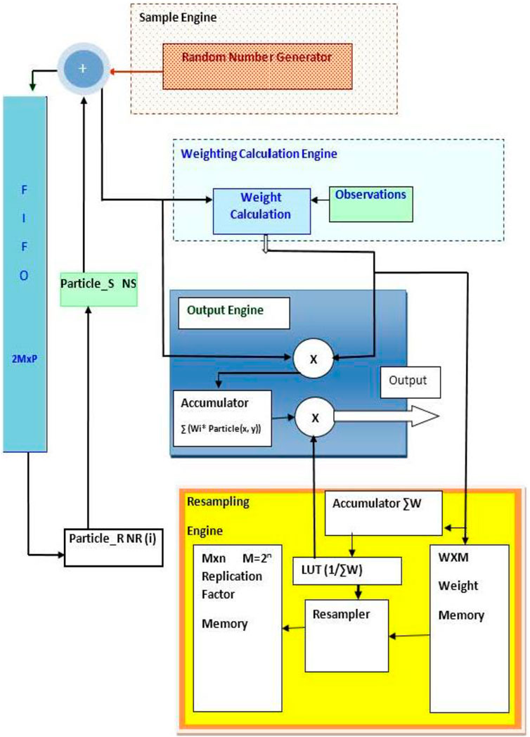
FIGURE 8. SIRF Localizer processor architecture.
The straightforward implementation of the output calculation is accomplished by employing two accumulators to sum each of x and y values for all particles, which is then multiplied by its weight and multiplied by the inverse value of the total weight.
4) After sampling the total number of particles is done, the resample process starts and gives a replication factor for each particle according to its weight using one of the resampling methods. The basic idea of resampling is to eliminate small-sized particles and concentrate on particles with large weights. The resampling process calculates sequentially the replication factor for each particle for the next instant. The resample calculates one replication factor for every clock cycle.
5.1.1 Sample Unit
Figure 9 shows a block diagram of the sampling unit. The sampling unit contains two random generators implemented using Hybrid Cellular Automata (CA) CA 150 and CA 90 rules (Abd el-hamid, 2008). The used CA consists of N alternating cells, which change their states according to rules 90 and 150. The Random Number Generator (RNG) uses XOR logic, implemented in VHDL, to calculate the next state of an indicated cell in the array.
FIGURE 9
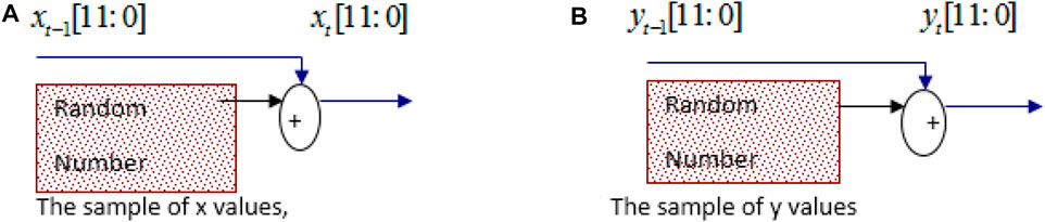
FIGURE 9. Sampling unit. (A) The sample of x values (B) The sample of y values.
The sample engine generates noise values added or subtracted to the particle state vector elements, stored in register Particle S, before saving it back to the FIFO for the next instant.
5.1.2 Weight Calculations
Our likelihood function was designed as a linear function for hardware simplification. Considering the complexity of the hardware implementation of the square root and the exponential function, we need to find the magnitude of a two-dimensional vector quickly without using a square root function. A common approximation takes the following form:
Where α= 0.94 and β= 0.39.
In hardware, we calculate the maximum term as (1-0.062) and the minimum term as (0.25 + 0.125), which is a good approximation. By using simple linear approximations, we may reduce the weighted function computations. Figure 10 compares the FPGA implemented weighting function with the true exponential function. Matlab simulation results indicate that this approximation does not affect the performance of the localizer. The exponential function also can be used as a lookup table when the maximum and minimum value are known. Figure 11A shows its implementation in MatLab. Figures 11B,C shows the schematic and simulation of VHDL implemented exponential function using fixed-point representation.
FIGURE 10
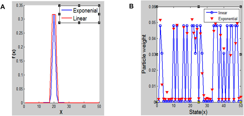
FIGURE 10. (A) Simplified function for the weight calculations. (B) Estimated value by a simplified process of the particle weight.
FIGURE 11
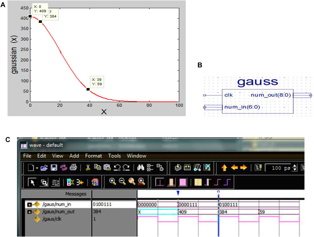
FIGURE 11. Exponential function (A) MatLab implementation (B) Schematic (C) Simulation.
To reduce the H/W resources requirements, all variables are used in fixed-point representation form. The average standard deviation of measurements of ref. (Abd el-Hamid, 2015) is scaled and used in the implementation.
5.2 Residual Resampling Algorithm
In Residual Resampling (RR), resampling is performed where the number of replications of a specific particle is determined in one loop by truncating the product of the number of particles, and the simple truncation may result in a total number of replicated particles less than M. In general, R = ∑r (m) may not be equal to M. For solving this problem, for example, if the sum of all replicated particles is less than, M the hardware must decide which particles to replicate additionally so that the total number of particles is constant.
In the RR algorithm, for M input and N output (resampled) particles, the summation of all particles replication factors are less than the input particles M (N < M). The difference between input and output is obtained using the mechanism (Abd El-Halym et al., 2012), in which we added this remainder number to the replication factor of the highest weight particle.
The replication of each particle is calculated as follows:
The simple structure of the resampling is executed by employing the lookup Table, which is used to calculate the inverse value of the weight summation, which lies between 1 and 64, then multiply this value by M. Accordingly, the number
5.2.1 Residual Systematic Resampling Algorithm
Systematic resampling (SR) is the most commonly used since it is the fastest resampling algorithm for computer simulations (Bolic et al., 2005). But it takes two loops of m iterations. In Residual Systematic Resampling (RSR), the updated uniform random number is formed differently, which allows for only one iteration loop and processing time independent of the distribution of the weights at the input (Bolic, 2004).
The RSR algorithm draws the uniform random number U(0) = ΔU(0) in the same way of SR but updates it by ΔU(m) = ΔU(m−1) + i(m)M − w(m)n. The uniform number is updated depending on the previous uniform number ΔU (m−1), calculated and then used as the initial uniform random number for the next particle. When trying to calculate ΔU (m), this uniform number is updated regarding the current weight. For these reasons, the RSR must be implemented sequentially and cannot be implemented in parallel. So, this resample approach is implemented in the proposed sequential architecture.
Figure 12 shows a simulation run illustrating the localizer using RSR and shows the time between every successive estimation values.
FIGURE 12
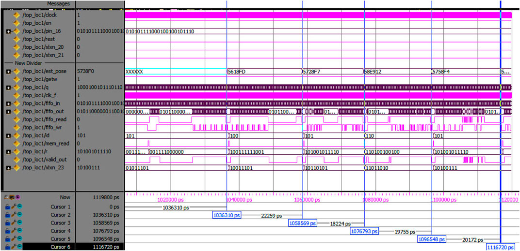
FIGURE 12. A simulation run that illustrates the operation of the localizer with RSR.
The Sequential resampling engine can be redesigned to work in parallel using several scenarios of parallel execution units, as shown in Figure 13. Considering data dependencies, this can be achieved by splitting the resampling process into multiple concurrent loops. When we use M loops, we consume the resources of the H/W implementation. The figure demonstrates the speed gain from using eight parallel resampling loops over a single loop.
FIGURE 13
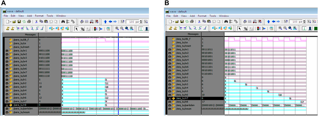
FIGURE 13. The execution time comparison (A) The eight parallel resampling loops give the replication factors at one clock cycle. (B) One loop (sequential) RSR replicates factors after M clock cycles for M = 8.
5.3 The Resources Utilization
The architecture is captured using VHDL and synthesized on a Xilinx Virtex 5 FPGA chip. Finally, the design is verified using ModelSim simulator. Table 4 summarizes the total resources utilization of the implemented architectures.
TABLE 4
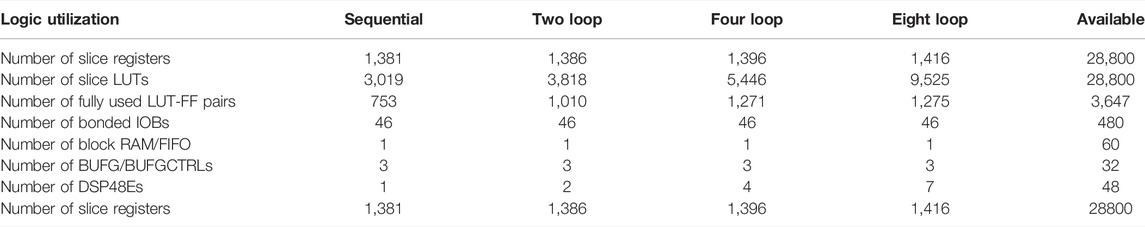
TABLE 4. The resources utilization for the implemented architecture of Sequential and parallel resampling on xc5vlx50t-3-ff1136 chip.
The proposed architecture uses two memory arrays: one MxW to store the weights of the particles where W equals to 8 bits used in our fixed-point representation and the other Mxn memory to store the replication factor where M = 2n FIFO is implemented as a circular queue, where data can be stored and retrieved (in the order of its entry only) and thus has a read pointer and a write pointer. A synchronous FIFO uses the same clock for reading and writing. Moreover, total memory requirements for this architecture are: one dual-port FIFO of 2M words to store the particles vectors of width equals 24 bits.
5.4 Analysis of Execution Time
The timing diagram of our proposed architecture operations is shown in Figure 14. Ti is the initial latency in particle generation, which equals two clock cycles. Therefore, the total cycle time required is TSIRF = (TW + Tres + αM) Tclk. The particle generation and computation weight operations can be overlapped in sequence such that TW is the startup latency of the weight calculation unit, which is equal to one clock. Therefore, the total latency cycles are three. Tres is the resampling time equal to M + 1 clock periods (one clock to add the M-N to the highest weight replication factor). In the routing of the particles, the value of α lies between 1 and 2 and depends on the replication factors of the particles. The best value α is 1, where every clock routs one particle such that the total routing time is M. The worst-case takes place when the first M−1 particles have zero replication factors. Only the last stored particle in the FIFO has a replication factor that equals M in this case; the FIFO needs to read M−1 particles first, till FIFO reaches the particle number M. Then the sampling, weighting, and the output calculations are started and repeated for those particle M times. For all other cases (when a considerable number of the particles have non-zero replication factors), the value of α is slightly more than one.
FIGURE 14
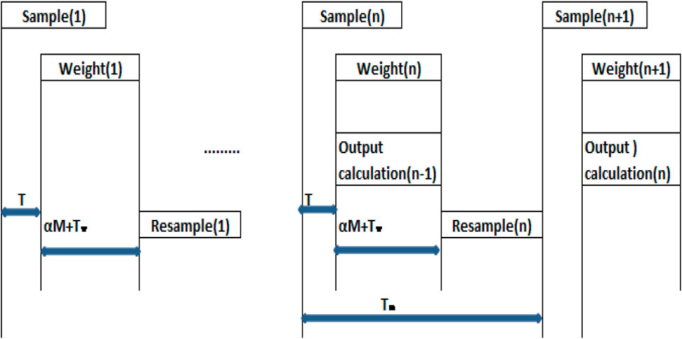
FIGURE 14. The timing diagram for the SIRF evaluation.
From the timing summary, the total time consumed for SIRF with RSR is 28.958 ns (maximum frequency: 34.533 MHz) using Xilinx FPGA chip xc5vlx50t with speed grade: -3.
Several architectures are implemented and compared to explain the tradeoff between speed up and resource utilization. The design occupies a small part of the targeted Xilinx chip. So, smaller and more affordable chips (e.g., Xilinx Zynq-7010) will be sufficient.
6 Conclusion
A proposed radioactive source localization algorithm is presented. Apollonius circle calculated range guides a Particle Filter for estimating the source location using actual measurements. The proposed algorithm outperforms the Iterative Pruning Clustering algorithm when using just four sensors and above. For sensor counts less than four, the results of the two algorithms are comparable. Furthermore, the proposed algorithm can localize a source, even when the area surrounded by the sensors does not contain that source. This case is unattained by all other approaches. A H/W implementation of this particle filter in a Xilinx FPGA chip is also presented. Several implementation architectures are evaluated. The selected architecture targets a balance between hardware resources and speeds up accomplished. The future work plan includes security-related studies and complete WSN implementation using μC/FPGA devices.
Data Availability Statement
The original contributions presented in the study are included in the article/Supplementary Material, further inquiries can be directed to the corresponding author.
Author Contributions
All authors listed have made a substantial, direct, and intellectual contribution to the work and approved it for publication.
Conflict of Interest
The authors declare that the research was conducted in the absence of any commercial or financial relationships that could be construed as a potential conflict of interest.
Publisher’s Note
All claims expressed in this article are solely those of the authors and do not necessarily represent those of their affiliated organizations, or those of the publisher, the editors and the reviewers. Any product that may be evaluated in this article, or claim that may be made by its manufacturer, is not guaranteed or endorsed by the publisher.
References
Abd el-Hamid, A. A. (2008). Optimum Motion Track Planning for Avoiding Obstacles. Cairo: Benha University. Available at: http://db4.eulc.edu.eg/eulc_v5/Libraries/Thesis/BrowseThesisPages.aspx?fn=PublicDrawThesis&BibID=10614401
Abd El-Halym, H. A., Mahmoud, I. I., and Habib, S. (2012). Proposed Hardware Architectures of Particle Filter for Object Tracking. EURASIP J. Adv. Signal. Process., 2012 (1), 1–19. doi:10.1186/1687-6180-2012-17
Abd el-Hamid, A. A. (2015). Locating a Mobile Robot in a Non_Accessible Area. Cairo: Benha University. Ph.D.
Arulampalam, M. S., Maskell, S., Gordon, N., and Clapp, T. (2002). A Tutorial on Particle Filters for Online Nonlinear/Non-Gaussian Bayesian Tracking. IEEE Trans. Signal. Process. 50, 174–188. doi:10.1109/78.978374
Baidoo-Williams, H. (2016). Maximum Likelihood Localization of Radiation Sources with unknown Source Intensity. Computer Science arXiv:Optimization and Control. Available at: https://arxiv.org/pdf/1608.00427.pdf
Bolic, M., Djuric, P. M., and Sangjin Hong, S. (2005). Resampling Algorithms and Architectures for Distributed Particle Filters). IEEE Trans. Signal. Process. 53 (7), 2442–2450. doi:10.1109/TSP.2005.849185
Bolic, M. (2004). Architectures for Efficient Implementation of Particle Filters. New York: Stony Brook University. Ph.D. thesis.
Chin, J-C., Yau David, K. Y., Rao Nageswara, S. V., Yang, Y., Ma, C. Y. T., and Shankar, M. (2008). Accurate Localization of Low-Level Radioactive Source under Noise and Measurement Errors. Computer Science Technical Reports. New York, NY: Association for Computing Machinery.
Chin, J.-C., Rao, N. S. V., Yau, D. K. Y., Shankar, M., Yang, Y., Hou, J. C., et al. (2010). Identification of Low-Level point Radioactive Sources Using a Sensor Network. ACM Trans. Sen. Netw. 7 (3), 1–35. doi:10.1145/1807048.1807050
Cook, J., Smith, R., Ramirez, C., and Rao, N. (2020). Particle Filtering Convergence Results for Radiation Source Detection. New York, NY: Association for Computing Machinery. Available at: https://arxiv.org/pdf/2004.08953.pdf.
Cordone, G. (2019). Improvements to MLE Algorithm for Localizing Radiation Sources with a Distributed Detector Network. M. Sc Thesis. South Carolina: Clemson University. Available at: https://tigerprints.clemson.edu/all_theses/3078.
Dalal, S. R., and Han, B. (2010). Detection of Radioactive Material Entering National Ports: A Bayesian Approach to Radiation portal Data, Ann. Appl. Stat. 4 (3), 1256–1271. doi:10.1214/10-AOAS334
Fox, D., Burgard, W., and Thrun, S. (1999). Markov Localization for Mobile Robots in Dynamic Environments. jair 11, 391–427. doi:10.1613/jair.616
Fragkos, G., Karafasoulis, K., Kyriakisand, A., and Potiriadis, C. (2020). Localization of Radioactive Source Using a Network of Small Form Factor CZT Sensors. J. Instrument. 15, C04015. doi:10.1088/1748-0221/15/04/c04015
Gunatilaka, A., Ristic, B., and Gailis, R. (2007). “On Localisation of a Radiological Point Source,” in 2007 Information, Decision and Control, Adelaide, SA, Australia, February 12–14, 2007. doi:10.1109/idc.2007.374556
Jarman, K. D., Miller, E. A., Wittman, R. S., and Gesh, C. J. (2011). Bayesian Radiation Source Localization. Nucl. Technol. 175 (1), 326–334. doi:10.13182/NT10-72
Kim, B. (2021). The Circle of Apollonius. Available at: http://jwilson.coe.uga.edu/EMAT6680Fa09/KimB/EMAT6690/Essay2/6690%20apollonius%20circle.pdf (last accessed 10 28, 2021).
Kyriakis, A., and Karafasoulis, K. (2020). "An AI Approach in Radioactive Source Localization by a Network of Small Form Factor CZT Sensors,” in SETN 2020 Workshops, Athens, Greece, September 02–04, 2020. Available at: http://ceur-ws.org/Vol-2844/
Liu, A. H., Bunn, J. J., and Chandy, K. M. (2011). “Sensor Networks for the Detection and Tracking of Radiation and Other Threats in Cities,” in Proceedings of the 10th ACM/IEEE International Conference on Information Processing in Sensor Networks, Chicago, IL, April 12–14, 2011 (Chicago, IL: IEEE), 1–12.
Liu, A. (2010). Simulation and Implementation of Distributed Sensor Network for Radiation Detection. Master of Science California.
Mahmoud, I. I., Salama, M., and El Hamid, A. A. E. T. A. (2016). “Hardware Implementation of a Genetic Algorithm for Motion Path Planning,” in Field-Programmable Gate Array (FPGA) Technologies for High-Performance Instrumentation, 250–275. doi:10.4018/978-1-5225-0299-9.ch010
Marimon, D., David, Y. M., Abdeljaoued, Y., and Ebrahimi, T. (2007). “Particle Filter-Based Camera Tracker Fusing Marker and Feature point Cues,” in Electronic Imaging 2007 (SPIE). doi:10.1117/12.703150
Rao, N., Shankar, M., Jren-Chit, C., Yau, D. K. Y., Yang, Y., Hou, J. C., et al. (2008). “Localization under Random Measurements with Application to Radiation Sources,” in information fusion,11th international conference, Cologne, Germany, June 30–July 3, 2008.
Rao, N. S. V., Sen, S., Cooper, N. J. D. A., Ledoux, R. J., Costales, J. B., Kamieniecki, K., et al. (2015). Network Algorithms for Detection of Radiation Sources. Nucl. Instr. Methods Phys. Res. Sect. A. 784, 326–331. doi:10.1016/j.nima.2015.01.037
Tandon, P., Huggins, P., MacLachlan, R., Dubrawski, A., Nelson, K., and Labov, S. (2016). Detection of Radioactive Sources in Urban Scenes Using Bayesian Aggregation of Data from mobile Spectrometers. Inf. Syst. 57, 195–206. doi:10.1016/j.is.2015.10.006
Wu, C. Q., Sen, S., Rao, N. S. V., Brooks, R., and November, (2014). “Efficient Network Detection of Radiation Sources Using Localization,” in IEEE Nuclear Science Symposium, Seattle, WA, USA, November 8–15, 2014.
Wu, C. Q., Berry, M. L., Grieme, K. M., Sen, S., Rao, N. S. V., Brooks, R. R., et al. (2019). Network Detection of Radiation Sources Using Localization-Based Approaches. IEEE Trans. Ind. Inf. 15 (4), 2308–2320. doi:10.1109/TII.2019.2891253
Zhang, T. (2012). “Radioactive Target Detection Using Wireless Sensor Network,” in Computer Informatics, Cybernetics, and Applications (Springer Science). doi:10.1007/978-94-007-1839-5_31
Keywords: wireless sensor networks, localization, radiation sources, security, particle filter, FPGA, hardware
Citation: Mahmoud II and Abd el-Hamid AA (2022) Particle Filter Based Range Search Approach for Localization of Radioactive Materials. Front. Energy Res. 9:807918. doi: 10.3389/fenrg.2021.807918
Received: 02 November 2021; Accepted: 31 December 2021;
Published: 31 January 2022.
Edited by:
Mingfei Yan, RIKEN, JapanReviewed by:
Zhiqiang Niu, Loughborough University, United KingdomBaolong Ma, Xi’an Jiaotong University, China
Copyright © 2022 Mahmoud and Abd el-Hamid. This is an open-access article distributed under the terms of the Creative Commons Attribution License (CC BY). The use, distribution or reproduction in other forums is permitted, provided the original author(s) and the copyright owner(s) are credited and that the original publication in this journal is cited, in accordance with accepted academic practice. No use, distribution or reproduction is permitted which does not comply with these terms.
*Correspondence: Imbaby I. Mahmoud, imbabyisma@yahoo.com