Ecological diversity methods improve quantitative examination of student language in short constructed responses in STEM

We novelly applied established ecology methods to quantify and compare language diversity within a corpus of short written student texts. Constructed responses (CRs) are a common form of assessment but are difficult to evaluate using traditional methods of lexical diversity due to text length restrictions. Herein, we examined the utility of ecological diversity measures and ordination techniques to quantify differences in short texts by applying these methods in parallel to traditional text analysis methods to a corpus of previously studied college student CRs. The CRs were collected at two time points (Timing), from three types of higher-ed institutions (Type), and across three levels of student understanding (Thinking). Using previous work, we were able to predict that we would observe the most difference based on Thinking, then Timing and did not expect differences based on Type allowing us to test the utility of these methods for categorical examination of the corpus. We found that the ecological diversity metrics that compare CRs to each other (Whittaker’s beta, species turnover, and Bray–Curtis Dissimilarity) were informative and correlated well with our predicted differences among categories and other text analysis methods. Other ecological measures, including Shannon’s and Simpson’s diversity, measure the diversity of language within a single CR. Additionally, ordination provided meaningful visual representations of the corpus by reducing complex word frequency matrices to two-dimensional graphs. Using the ordination graphs, we were able to observe patterns in the CR corpus that further supported our predictions for the data set. This work establishes novel approaches to measuring language diversity within short texts that can be used to examine differences in student language and possible associations with categorical data.

1. Introduction

1.1. Assessment of student thinking in STEM through constructed response

Assessment of student understanding and skills is an essential component of teaching, learning, and education research. For this reason, science education standards have pushed for increased use of assessment practices that test authentic scientific practices, such as constructing explanations, and assessments that measure knowledge-in-use (NGSS Lead States, 2013; Gerard and Linn, 2016; Krajcik, 2021). Constructed responses (CRs) are an increasingly used type of assessment that provide valuable insight to both instructors and researchers, as students express their understanding or demonstrate their ability using their own words (Birenbaum et al., 1992; Nehm and Schonfeld, 2008; Gerard and Linn, 2016). Through CRs, students reveal differing levels of performance, complex thinking, and unexpected language in a variety of STEM topics including evolution (Nehm and Reilly, 2007), tracking mass across scales (Sripathi et al., 2019), statistics (Kaplan et al., 2014), mechanistic reasoning in chemistry and genetics (Noyes et al., 2020; Uhl et al., 2022), and covariational reasoning (Scott et al., 2022). Due to their value and expanded use, it is increasingly important for assessment developers and researchers to have methods to carefully and quantitatively examine the language within CRs. Such methods could allow for comparison of expert and novice language, determine if substantial differences in student language occur due to instruction, regions or institutional type, or help examine bias in written assessments. Unfortunately, quantitative methods of examining and comparing the words within corpuses of short texts, such as CRs, are limited.

1.2. Current methods of written language analysis and their limitations

Text analysis falls into two major categories: qualitative and quantitative. For qualitative text analysis, researchers typically use “coding,” in which expert coders categorize “the text in order to establish a framework of thematic ideas about it” (p. 38; Gibbs, 2007). Coding is the most common approach for qualitative analysis in content based CRs in STEM, as it gives insight into student thinking by examining student produced text or words. In previous work with CRs, coding has reflected various frameworks in STEM, including cognitive models such as learning progressions (Jescovitch et al., 2021; Scott et al., 2022), the use of scientific skills (Uhl et al., 2021; Zhai et al., 2022), or the presence of key conceptual ideas (Nehm and Schonfeld, 2008, Sripathi et al., 2019; Noyes et al., 2020). Qualitative coding can be done by reading the responses or using text mining programs that use computer-based dictionaries and natural language processing to pull out themes from the text. Through these qualitative methods, researchers often observe words or phrases that are associated with the coding of the text. These observations can often be statistically supported using quantitative analysis. Quantitative text analysis is typically performed via content or dictionary analysis, in which the text is reduced to word and phrase frequency lists that can be examined and/or compared between CRs or groupings of the CRs that are based on the qualitative coding. These types of analyses can be useful; however, these approaches do not examine the CRs holistically or examine the diversity of language used. While dictionary analysis allows for comparison of individual words or phrases between groups, this analysis seems overly reductive, since the words and phrases are typically interpreted as a part of the overall response by human coders. To assist with this gap, machine learning and natural language processing have also been used to better analyze texts for meaning (Boumans and Trilling, 2016). One approach currently used in text analysis to holistically examine language is through latent semantic analysis (LSA). LSA uses natural language processing and machine learning to compare the language in different texts to each other based on the words within the texts (Deerwester et al., 1990; Landauer and Psotka, 2000). While this method and others related to it have been used to help identify themes in CRs (Sripathi et al., 2019) and even in the creation of computer scoring models for automated analysis of student thinking (LaVoie et al., 2020), their purpose is to identify meaning or common topics in the text. The identified themes or topics must be interpreted for relevance by an expert in the domain. In contrast, we are interested in comparing and quantifying the diversity of words students use in written explanations.

Our interest in comparing the words students use could also be approached through lexical diversity, which measures the range of words in a given text, with high lexical diversity values indicating more varied language (Jarvis, 2013). Many lexical diversity measures, most commonly Type to Token (TTR) and several derivatives, calculate the proportion of words in a text that are unique. These measures are helpful predictors of linguistic traits, including vocabulary and language proficiency (Malvern et al., 2004; Voleti et al., 2020). Unfortunately, these lexical diversity measures cannot be applied to CRs, as many are sensitive to the text length and cannot be applied to texts under 100 words (Tweedie and Baayen, 1998; Koizumi, 2012; Choi and Jeong, 2016). Although some lexical diversity measures, such as MATTR (Covington and McFall, 2010; Zenker and Kyle, 2021), allow use of shorter texts of 50–100 words, most content-based CRs in STEM can frequently be as short as 25–35 words (Haudek et al., 2012; Shiroda et al., 2021). Beyond the length requirement, we find these lexical measures somewhat lacking for our intended use in that they do not present a full picture of diversity, as they only measure the repetition of words within a single response. In contrast to linguistics for which repetition does often indicate language proficiency, word repetition is not necessarily indicative of proficiency in STEM assessments. This could be especially true when considering the importance of discipline specific language which restricts word choice. In particular, we are interested in holistically comparing responses to one another based on word frequency. Such an approach could be used to determine if certain variables (e.g., question prompt, timing) are associated with more similar or varied language in student CRs.

Quantifying such diversity between two CRs or within a group of CRs is more similar to measures of ecological diversity than any current form of text analysis. Indeed, Jarvis (2013) previously compared lexical diversity to ecological diversity (ED) approaches and proposed applying ecological definitions and practices to texts. Within his work, Jarvis comments, “Both fields view diversity as a matter of complexity, but ecologists have gone much further in modeling and developing measures for the different aspects of that complexity. Ecologists have also held to a literal and intuitive understanding of diversity, and this has resulted in a highly developed, intricate picture of what diversity entails.” (p. 99; 2013). Indeed, ED metrics quantify not only diversity within a sample but between samples within data sets. Further, ecologists also commonly use a data reduction technique called ordination to explore data sets and test hypotheses. To our knowledge, this idea of applying ecological methods to language has never been empirically tested and its application to a corpus of short, content rich CRs is novel.

1.3. Ecological diversity metrics

In ecology, Robert Whittaker articulated three diversity metrics that are now central to ecology: alpha, gamma, and beta diversity (Figure 1A, Whittaker, 1972). Alpha (α or species richness) diversity is the count of the number of species in a sample. This idea is similar to counting unique words (also called Types in lexical diversity) in a CR. For example, as shown in Figure 1A, Sample A has a higher alpha than Sample B. Both samples have 4 individuals, but all four in A are unique, while Sample B has three of the same species. Gamma (γ) is the count of the total number of species in a pair or set of samples, similar to the total words (also called Tokens in lexical diversity) in a CR. Beta diversity (β) compares the species occurrences between samples (Whittaker, 1967, 1969) and does not have an equivalent in lexical diversity or text analysis. This is the simplest calculation of β diversity; however, other metrics can be used to represent this kind of relatedness, including absolute species turnover (Tuomisto, 2010; McCune and Mefford, 2018). The species turnover measure uses presence-absence data of species in samples and is considered a better indicator of relatedness than β, as β can be heavily affected by rare species (Vellend, 2001; Lande, 1996). Another method of comparing two or more samples is using dissimilarity measures, such as Bray–Curtis dissimilarity (Bray and Curtis, 1957). This is calculated by comparing every pair of species within two samples. While these measures may appear redundant, each can be biased in different ways (Roswell et al., 2021). Examining a collection of diversity metrics results in a more equitable description of the data, in much the same way that mean, median, and mode all offer different values for a measure of central tendency (Zelený, 2021).

FIGURE 1

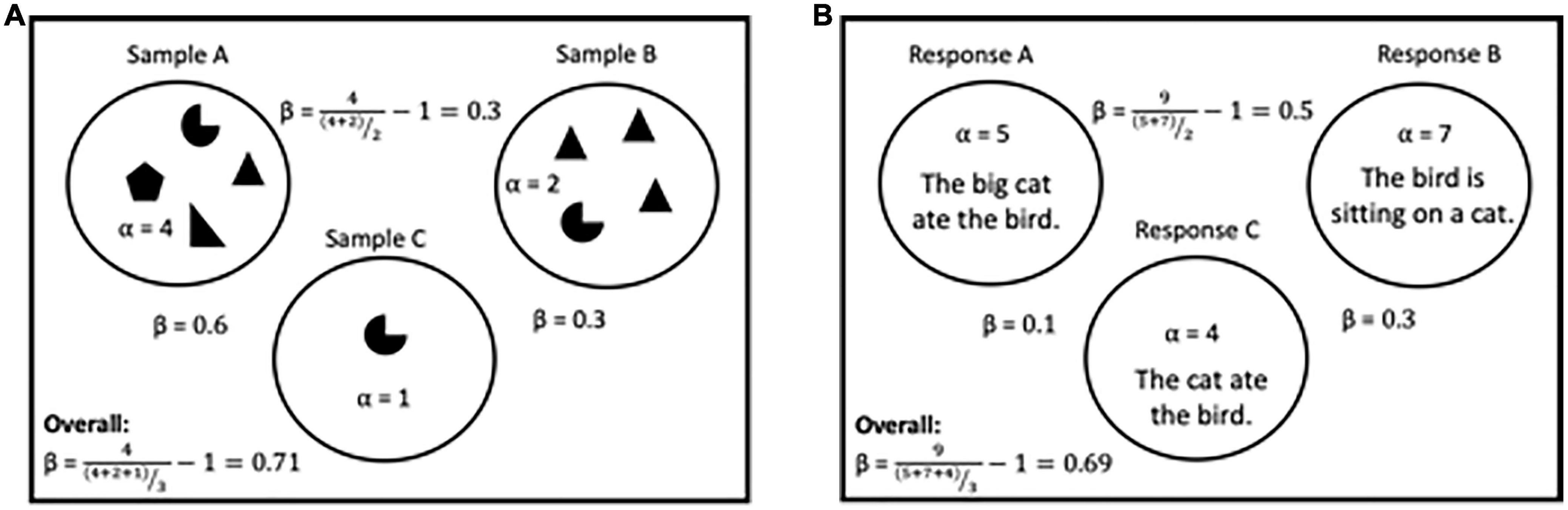
Figure 1. Schematics of ecological diversity terms. (A) For ecological diversity, three samples (open circles) are shown with differing numbers of individuals, representing a different species (filled shapes). Alpha values are given for each sample, and beta values are given for each pairing and the overall data set. Example calculations are provided for beta between Sample A and B and the data set overall. (B) For language applications, responses are compared instead of samples, while words are treated as individuals. Repeated words are equivalent to being the same species. While only single sentences are shown here, our data set contains many CRs that contain more than one sentence that are still treated as single samples. Alpha values are given for each response, and beta values are given for each pairing and the overall data set. Example calculations are provided for beta between response A and B and the data set overall.

In addition to comparing species between samples, other measures examine the diversity of individual communities or samples. These types of measures include Evenness (E), Shannon’s diversity index (H’; Shannon, 1948) and Simpson’s diversity index (D; Simpson, 1949). Evenness describes the proportional abundance of species across a given sample and indicates if a sample is dominated by one or a few species. Similar to Whittaker’s β, species turnover and Bray–Curtis Dissimilarity, H’ and D both represent the diversity of a single community or sample but are calculated slightly differently. H’ represents the certainty of predicting a single species of a randomly selected individual, while D is the probability of two random species being the same. Each measure has potential biases associated with it, resulting in most researchers examining both metrics for a clearer picture of the data (Zelený, 2021).

1.4. Ecological diversity visualization

In addition to diversity metrics, ecological studies also apply ordination methods to visualize and extract patterns from complex data (Gauch, 1982; Syms, 2008; Palmer, n.d.). Ordination methods use dimension reduction to project multivariate data into two or three dimensions that can be visualized in a map-like graph. This technique arranges samples with greater similarity more closely to each other as points in the graph, while samples with lower similarity are further apart. These ordination methods are often used in combination with ED metrics as the ordination techniques provide unique benefits. First, diversity is complex in a way that an individual measure or even a collection of measures do not fully relate to the whole of an object. Jost (2006) said, “a diversity index itself is not necessarily a ‘diversity.’ The radius of a sphere is an index of its volume but is not itself the volume and using the radius in place of the volume in engineering equations will give dangerously misleading results” (p. 363). Ordination attempts to collapse the diversity in a different way compared to ED metrics through extracting patterns while attempting to account for as much variation in the data as possible. Second, extracting and prioritizing patterns that best explain the data focuses researchers on the most important patterns, allowing them to ignore noise in the data. Ecologists have found that even if ordinations result in a low percentage of variance in the data being explained, the ordinations are still meaningful and, more importantly, provide insight into the system being studied (Goodrich et al., 2014). Third, different patterns can be observed when a data set is examined holistically as opposed to examination of categorical sub-groups. In comparison, ED metrics need to be calculated by defining subsets of the data to obtain a single value for categorical data, while ordination analysis is performed on the entire data set and categorical data is overlaid. Finally, ordination results in an intuitive graph whose patterns can be more easily interpreted to better understand communities and how they relate to each other. For these reasons, ordination is used in diverse fields including image analysis, psychology, education research, and text analysis. Within education research, Graesser et al. (2011) used ordination to examine attributes of long texts in order to curate reading assignments for students. Borges et al. (2018) proposed the use of ordination to predict student performance and gain understanding of important student attributes, while another group used ordination to create models to evaluate teacher quality (Si, 2006; Xian et al., 2016).

For any of these applications, a data matrix is created that contains the objects of interest as rows and their attributes as columns. In ecological work, the matrix contains rows as samples and columns are species recorded in these samples (Figure 2A). The species in each row are compared for every pair in the matrix, resulting in a pairwise comparison of the entire matrix. The resulting distance or similarity values are a necessary prerequisite for distance-based ordination methods [ex: principal coordinate analysis (PCoA)] and eigen analysis-based methods [ex: detrended correspondence analysis (DCA)], both of which we use in this work. The patterns found in these data are used to create a map-like visualization that projects the distances or similarities between samples in two or three dimensions. While the idea of ordination is maintained, different methods of ordination vary in how they work. Each has their own strengths and weaknesses; therefore, it is common in ecology to apply multiple ordination methods in order to strengthen the conclusions made via one method. Selection between the different methods is based on the overarching question being investigated, the qualities of the data matrix, and the advantages or disadvantages of each method (Peck, 2010; McCune and Mefford, 2018; Palmer, 2019). Ordination methods fall into two general categories: indirect (unconstrained) and direct (constrained) methods (Syms, 2008). Indirect ordination is used to explore data for patterns from a species matrix (described above), while direct ordination is used to test if patterns in the species matrix are attributable to a secondary matrix of data (measured environmental factors associated with samples). In general, indirect ordination is considered exploratory and is used to generate hypotheses, while direct ordination is confirmatory and used to test hypotheses. Since we want to use ordination methods to explore our data set, we selected only indirect methods of ordination. When selecting a specific ordination method, it is important to recognize the limitations of the method and the data itself. For example, many ordination methods, including Principal Component Analysis (PCA) and Non-metric multidimensional scaling (NMDS), do not handle high numbers of zeros in the data set well (Peck, 2010). However, high-zero data exists in many instances, and methods exist to circumvent this limitation, including DCA and PCoA.

FIGURE 2

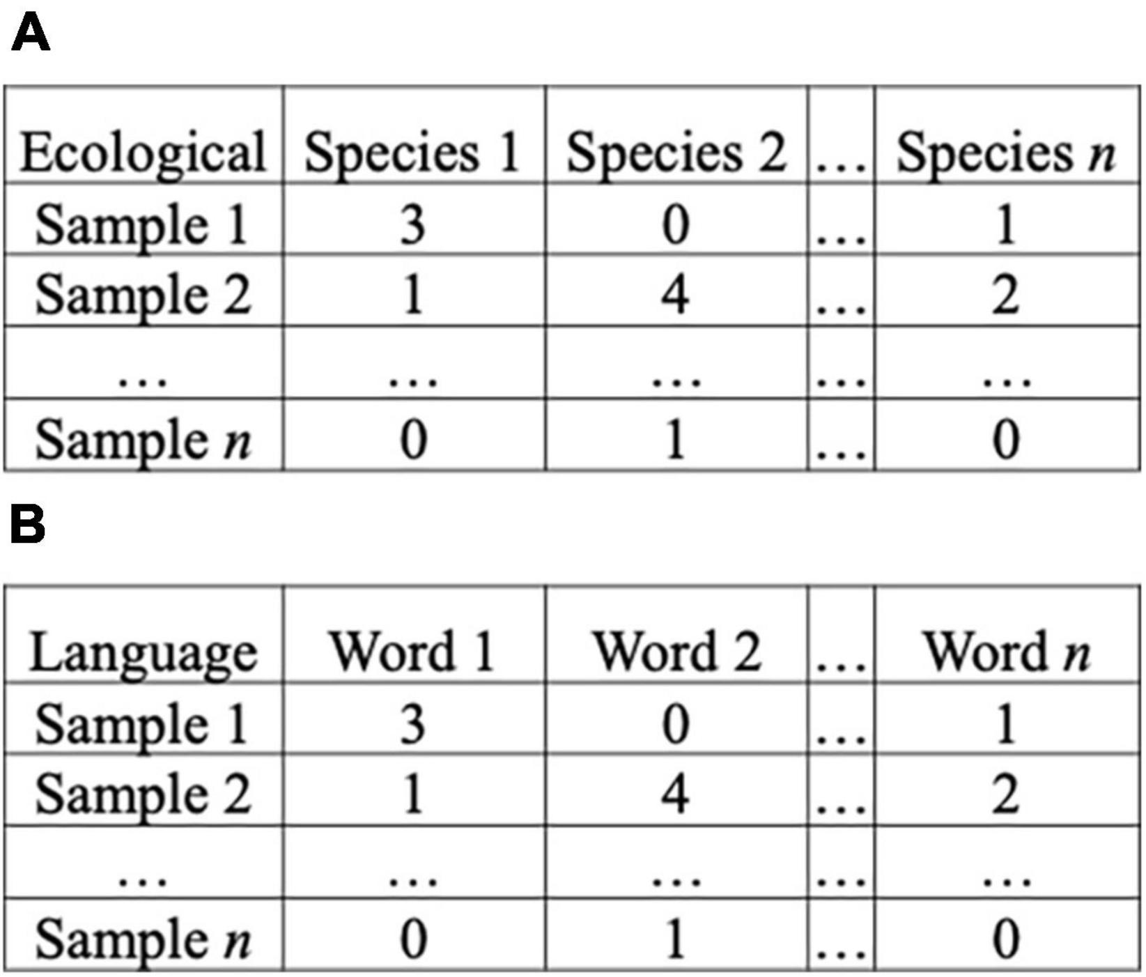
Figure 2. Sample matrices. (A) For ecological data matrices, samples are rows, while species are columns. Values in individual cells are the frequency of the given species in the sample. (B) In this example, each response is a row, while each word is a column. Values in cells are the frequency of a word within the response.

1.5. Applying ecological methods to language analysis and its potential benefits

Addressing the challenge of language analysis and comparisons for short texts, we propose applying ecological methods of diversity analysis to a corpus of CRs, in which each individual response is equivalent to a sample, and each word is analogous to a species within that sample. In Figure 1B, each response is a single sentence; however, in our data set, CRs can range from one word to multiple sentences. They are still counted as a single CR. Similarly, for each of the measures described above, we substitute the species with unique words in a single CR. With this application, α is the count of unique words in a CR and γ is the total abundance of words in a pair or larger grouping of responses. β diversity reflects differences in word inclusion between two responses (Figure 1B). H’ and D are similar to the lexical diversity measures (e.g., TTR and its derivatives) described above. However, in contrast, H’ and D do not have specific cutoffs for their use with smaller sample sizes (i.e., number of words in a CR). Low alpha data sets are common in ecology as some environments do not support a large variety of species (e.g., Roswell et al., 2021). Similarly, it is common to observe large differences in α within ecological samples. These differences are often accounted for using a standardization method, such as equalizing effort, sample size or coverage. In this work, we are using an equalizing effort approach in that each student was presented the same opportunity (assessment item and online text box) to supply their CR (sample). However, it is important to note that ED metrics are still sensitive to α as many are calculated using α either directly or indirectly. They should therefore be interpreted carefully if there are stark differences in α. In addition to offering a solution to the length requirement of lexical diversity measures, Whittaker’s β, species turnover, and Bray–Curtis Dissimilarity allow holistic comparison of the CRs to each other in a way that no current text analysis methods do.

Ordination methods add to this holistic comparison by visualizing language differences in the CR corpus. To accomplish this, each CR is a row in our matrix and each column is the frequency of that word in the CR, similar to a term-document matrix in text analyses (Figure 2B). The nature of a large corpus of CRs results in a high number of zeros as the majority of words are used infrequently, resulting in a sparse data set. The high percentage of zeros results in a non-normal distribution of the data, restricting the ordination methods that can be used. However, these types of data sets are increasingly common with microbial diversity studies, which established best practices for sparse data sets, including Principal Coordinate Analysis (PCoA). We elected to use this method because it is most commonly used for sparse data but note one potential drawback in its utility for language diversity in comparison to an ecological study. PCoA ignores zero-zero pairs (when two separate rows being compared each have matching zero values). In ecology, zeros can mean that a species was not detected or that the species is truly not present, making it, in a way, favorable to ignore them. In comparison, with language a zero represents a known absence, and this absence can be as important as its presence. To ensure ignoring zero-zero pairs does not drastically change the observed patterns, we also applied another ordination approach. DCA is one of the most widely used methods in ecology (Palmer, 2019, Palmer, n.d.). This method is a type of Correspondence Analysis (CA) that reduces the dimensionality of a data set with categorical data. In addition to handling sparse data, this method has an additional benefit for our purposes as the x-axis is uniquely scaled in beta-diversity units, which allows users to calculate species turnover. In combination, DCA and PCoA complement each other and provide unique approaches that together support the results of the other. These approaches to diversity are similar to other types of text analysis techniques, including LSA described above, which can be visualized using ordination techniques similar to those described above. An important difference is that these DCA and PCoA techniques do not attempt to extract meaning from the texts and instead compare and contrast responses based solely on word frequencies without any weighting or dictionaries. This distinction is important to our goals because we are interested in measuring language diversity, not meaning.

Finally, in addition to the methods themselves, we appreciate the approach of ecology in interpreting diversity. Specifically, each metric is treated as a single view of the diversity, meaning that interpretation of diversity is done by taking into account each measure to provide a more comprehensive picture (Jost, 2006). This multifaceted approach will allow for full appreciation of the diversity of language students use in STEM CRs and will be more likely to reveal differences observed based on categorical data.

1.6. Present study

To test the application of ecological methods in analysis of short CRs, we utilized a corpus of 418 explanatory CRs collected from undergraduates that explore student understanding of the Pathways and Transformations Energy and Matter (American Association for the Advancement of Science, 2011) within the context of human weight loss. The question asks “You have a friend who lost 15 pounds on a diet. Where did the mass go?” We chose this data set as we have worked heavily with it and are very familiar with the language within the student CRs. Additionally, this corpus has three types of categorical data that can be used to test the method’s ability to find differences in corpus based on word usage, as we have expectations on which categories are likely to have different language. First, the CRs were previously coded for the presence or absence of seven ideas, categorized as normative (correct) or non-normative (naïve) (Table 1; Sripathi et al., 2019). Using the presence and absence of these ideas, the CRs can be further categorized into Developing, Mixed, or Scientific Thinking (Sripathi et al., 2019). We expect this categorization to result in the greatest difference in language as the ideas in the CRs should directly reflect the ideas written by students. In addition, these CRs were collected before and after an online tutorial on cellular respiration (Timing), and from three different institutional Types (Shiroda et al., 2021; Uhl et al., 2021). We have previously found that student performance was affected by engaging with the tutorial (Uhl et al., 2021) and therefore expect some differences in language to be observed based on Timing. In previous work, we did not observe striking differences in student ideas based on the institutional type [i.e., Research Intensive Colleges and Universities (RICUs); Primarily Undergraduate Institutions (PUI), and Two Year Colleges (TYCs)]; therefore, we are expecting these categories to result in the lowest language differences in this analysis.

TABLE 1

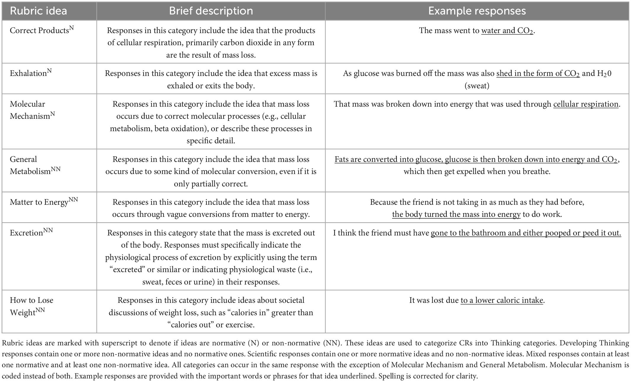
Table 1. Coding rubric and description.

In this paper, we apply common text analysis techniques to support our expectations that these three categorizations (Thinking, Timing, and Types) have varying amounts of difference in student language. Next, we outline the various methods and ED measures we applied to examine differences in short texts and demonstrate which ED methods reflect the differences in the categorical data to support their use in the analysis of short texts.

2. Materials and methods

2.1. Constructed response (CR) corpus collection and description

CRs were collected in collaboration with the SimBiotic Company as described by Uhl et al. (2021). Subsequently, Shiroda et al. (2021) examined a subset of 418 student responses. These studies were considered exempt by an institutional review board (x10–577). Briefly, college students enrolled in biology courses were asked to write a response to the prompt “You have a friend who lost 15 pounds on a diet. Where did the mass go?” in an online system. The subset of CRs used by Shiroda et al. (2021) and in this study are from 239 students from 19 colleges and universities across the USA. Shiroda et al. (2021) grouped the colleges and universities into three general categories of institutional type: Two Year Colleges (TYCs; n = 137), Primarily Undergraduate Institutions (PUIs; n = 142), and Research-Intensive Colleges and Universities (RICUs; n = 139). This information is reflected in the categorical data as Type. Students answered the prompt both before (n = 205) and after (n = 213) completing an online tutorial on cellular respiration. This information is reflected in the categorical data as Timing. For this study, we required that each response had at least one idea assigned to it (described below) to be included in the study. Therefore, student responses are not paired pre- and post-tutorial.

As part of previous work, Shiroda et al. (2021) coded these CRs using a rubric previously described by Sripathi et al. (2019; Table 1). Each response is dichotomously scored for each of the seven ideas, to indicate the presence (1) or absence (0) of the underlying idea in the rubric (described below). Briefly, a previous study validated ideas predicted for each response using a machine-learning model. As part of that validation process, an expert (MS) with a Ph.D. in biology independently assigned ideas using the rubric for the full set of 418 responses. Human and computer assigned ideas were then compared; any disagreements between human and computer ideas were examined by a second coder (KH) with a Ph.D. in biology. The two human coders discussed all human-human disagreements until agreement was met between the two human coders. The full coding procedure and validation are detailed further in Shiroda et al. (2021). This produced a data set with each response having values for seven ideas (i.e., a zero or one for each of seven ideas).

The applied rubric targets seven common ideas used by college students in response to the assessment item: Correct Molecular Products (carbon dioxide and water), physiological Exhalation (the weight leaves the body via exhalation in the form of carbon dioxide and water), and Molecular Mechanism (cellular respiration), General Metabolism, Matter Converted to Energy, How to Lose Weight, and Excretion (described further in Table 1). The first three ideas (underlined) are normative or scientific. The last four (italics) are non-normative or naïve ideas, in that they are not a part of an expert answer (Sripathi et al., 2019). All ideas can co-occur within the same answer, except General Metabolism and Molecular Mechanism. Molecular Mechanism is more specific than General Metabolism; therefore, Molecular Mechanism is coded in preference to General Metabolism if they both occur in the same CR.

Using these seven ideas, CRs were further categorized into one of three exclusive Thinking groups (Developing, Mixed, or Scientific) based on the inclusion of ideas associated with normative and non-normative ideas (Sripathi et al., 2019). This information is reflected in the categorical data as Thinking. Briefly, Developing responses contain one or more non-normative ideas and no normative ones (n = 181). Scientific responses contain one or more normative ideas and no non-normative ideas (n = 88). Mixed responses contain at least one normative and at least one non-normative idea (n = 149). Responses that have none of the seven coded ideas were not included in the study.

2.2. Text analysis

We compared the frequencies of words within categories of CRs between or among the categories of data (Thinking, Timing, or Type) in WordStat (v.8.0.23, 2004–2018, Provalis Research). We used the default program settings including a Word Exclusion list which removes common words and a preprocessing step of stemming (English snowball). Stemming removes the end of a word in order to mitigate the effect of different tenses, singular/plural, and common spelling errors. Words that have undergone stemming are noted in the text as the stemmed root with a dash (e.g., releas-). We did post processing of the text to keep only words with a frequency greater than or equal to 30 in the whole data set, and a maximum of 300 words were kept based on TF-IDF. TF-IDF stands for Term Frequency–Inverse Document Frequency and is a common statistic in text analysis used to reflect the importance of a word in a corpus. This measure weights words based on how much they are used but also accounts for those that are consistently used, meaning conjunctions and articles are not prioritized (Rajaraman and Ullman, 2011). In combination, these are the default settings in WordStat and are a way of focusing the results and preventing finding arbitrary, unmeaningful statistical differences based on chance (Welbers et al., 2017). Significance was determined by tabulating case occurrence in each grouping using a Chi-square. Words with p < 0.05 were considered significant.

2.3. Calculations and ED measures

All ED metrics were calculated in PC-ORD (version 7.08; McCune and Mefford, 2018). An ecological example of these calculations is provided in Figure 1A, while Figure 1B provides a text example. For the work presented in the body of the work, words were stemmed using Snowball (English) to limit the effect of tense. Misspellings were not corrected. No words were excluded. Other processing settings that we tried are described below. The resulting raw matrix has 418 rows (responses) and 694 columns (words).

Richness (S or α) is the number of non-zero elements in a row, or the number of unique words within a single response. Values provided for a categorical group are the averaged values for each response for the group.

Evenness (E) is a way of determining if a species (or word) is more common in an environment (or CR). In other words, a sample that is heavily dominated by a given species or word has a low evenness (0), while a sample that has the exact same frequency of each word has an evenness of 1. For example, in Figure 1A, samples A and C have an evenness of 1 as they are exactly the same. In contrast, sample B is more dominated by triangles, resulting in a lower evenness value. This calculated using the following equation:

$E=\frac{H^{\prime }}{ln(S)}.$

Beta diversity (β) compares the species occurrences between samples (Whittaker, 1967, 1969). A low β value indicates that two samples are very similar in species content, while a high β value indicates two samples are very different. This calculated using the following equation (PC-ORD version 7.08; McCune and Mefford, 2018; Figure 1A):

$B=\frac{\gamma }{\alpha }-1.$

In cases where the researcher wishes to compare β between three or more samples, we divide γ by the mean of α for all samples. The resulting value is β of all samples and represents how many samples there would be if γ and α per sample did not change, and all the samples share no species in common.

Species turnover (also called Absolute Species Turnover or half-change) represents the amount of difference between two samples. A value of one represents 50% of the species being shared and the other 50% being unique. Ecologists often use the term “half-change” to describe this condition. At two half-changes, 25% of species are shared between two samples. At four half-changes, the two samples are said to essentially not share any species. In contrast to β, there is not a simple relationship between species turnover and S. Species turnover can still be affected by S, but the relationship between the two can be either positive or negative (Yuan et al., 2016). Species turnover is calculated by the formula:

$\left(s_1-c\right)+\left(s_2-c\right),$

where s₁ is the number of words in the first CR, s₂ is the number of words in the second CR, and c is the number of words shared by both CRs (PC-ORD version 7.08; McCune and Mefford, 2018).

Bray–Curtis dissimilarity (or Sorensen dissimilarity) is a measure of percent dissimilarity. This measure ranges from 0 to 1, with 0 indicating two samples share all the same species. It is calculated using the formula:

$1-\frac{2W}{A+B},$

where W is the sum of shared abundances and A and B are the sums of abundances in individual responses (PC-ORD version 7.08; McCune and Mefford, 2018).

Shannon’s diversity index (H’) represents the certainty of predicting a single species of a randomly selected individual. This can be affected by both Richness (α) and Evenness. For example, if a sample contains only one species, the uncertainty of selecting that species is 0. This uncertainty can increase in two ways. First, uncertainty increases as more species are added (Figure 1A; sample A vs. C) or by changing evenness (sample A vs. B). If a community is dominated by a single species (low Evenness), it becomes more certain that the dominant species will be selected, thereby decreasing H’. It is therefore important when interpreting this measure that both richness and evenness be considered. Generally, this measure is more affected by richness than evenness (Zelený, 2021). While not depicted in the figure, H’ would be calculated individually for Responses A, B, and C and then averaged to obtain a value for a category of responses or the corpus as a whole (Jurasinski et al., 2009). H’ is calculated using the formula:

$-\sum Pi\times ln(Pi),$

where Pi is the proportion of the i-th word in the entire data set (Shannon, 1948).

Simpson’s diversity index (D) is the probability that two randomly selected individuals will be the same species. The probability of this decreases as richness increases and increases as evenness decreases (Zelený, 2021). As with H’, D would be calculated individually for Responses A, B, and C and then averaged to obtain a value for a group of CRs (Jurasinski et al., 2009). In comparison to H’, D is more influenced by evenness than richness. This is calculated using the formula:

$1-\sum Pi\times Pi,$

where Pi is the proportion of the i-th word in the entire data set (Simpson, 1949). The value of Simpson’s D ranges from 0 to 1, with 0 representing maximum diversity, and one denoting none. As a larger value represents a lower diversity, this is often presented as the inverse Simpson Index, which is calculated by dividing 1 by D. These values are provided in Supplementary Table 1.

2.4. Ordination techniques

Ordinations were performed using a curated word matrix that was created using a custom word exclusion list (containing articles, conjunctions, and prepositions) to reduce the number of uninformative, but frequent words (Table 2) in the raw matrix described above. We chose to exclude these words to focus the ordination analysis on informative language, pertinent to the science ideas, in the responses. We also excluded any words that did not occur in at least three responses, as patterns cannot be detected with a lower frequency and these words likely represent very infrequent ideas or ways students use ideas in our corpus. The resulting final data matrix or term-document matrix for ordination contained a total of 254 words (columns) and 418 responses (rows). We performed DCA and PCoA in PC-ORD (version 7.08; McCune and Mefford, 2018). Depending on the data set, some ecologists will transform the raw data in order for it to be used with certain methods. As we selected methods designed to work with our data set, we did not perform any transformations. The calculations needed to perform ordination techniques are performed within the software package in which several settings need to be selected. First, ordinations are calculated using a seed number which can be randomly selected or entered. Each seed number results in similar patterns, but with slightly different numbers; therefore, we selected the seed number 999. This ensures that the exact ordination calculations can be repeated. For DCA, we elected to down-weight rare words due to the large size of the data set. This focuses the ordination on overarching patterns in the data. For PCoA, a distance measure has to be selected. Similar to ordination itself, each measure has positive and negative attributes. We selected Bray–Curtis distance as it is optimal for non-normal data (Goodrich et al., 2014). Scores were calculated for words using weighted averaging. We examined the significance of each axis using 999 randomizations. The percent inertia (or variance explained) for each axis is provided in the outputs of the PC-ORD file and included in our results. We compiled categorical data (Type, Timing, and Thinking) associated with the CRs into a separate secondary matrix for ordination and used this secondary matrix with PC-ORD software to visually distinguish data points of different categories to help further reveal patterns of (dis)similarity in the data. DCA ordinations were then visualized using the R software package “phyloseq” (McMurdie and Holmes, 2013). Ellipses marking the 95% multivariate t-distribution confidence intervals were added to increase readability. PCoA ordinations were visualized in PC-ORD.

TABLE 2

Table 2. Words removed for ordination analysis.

2.5. Testing of other text processing protocols for ED metrics and ordination

For the ED metrics and ordinations, we also generated raw matrices using lemmatization (in place of stemming) and correcting misspellings from CRs, as these approaches are also common in the field of lexical analysis. We supply results from this other trial in Supplementary Table 2. Overall, results from these other text processing methods resulted in similar patterns for the ED metrics further described in the Results from stemming and no misspelling correction. For ordination, we also tested multiple word exclusion lists and frequency thresholds. Our trials included using the Default Exclusion list from WordStat, removing only “a, and, in, the” and the custom exclusion list provided in Table 2. We also tested frequency thresholds of 3 (minimum needed for pattern), 5 (present in 1% of responses), 22 (present in 5% of responses), and 50 (present in 10% of responses). Finally, we also tested using the raw matrix without any text processing. Each of these combinations resulted in a different number of words within the matrix, ranging from only 20 to 898 words (data not shown). When performing the ordination on these matrices, it affected the inertia explained but not the patterns in the graphs (data not shown). We selected the setting used herein as it was a middle number of words (264) and seemed to be the most representative of the language in the responses. However, others may choose a different exclusion list or frequency threshold, depending on their application.

2.6. Statistical analysis

PERMANOVAs (PERmutational Multivariate ANalysis Of VAriance) were calculated in PC-ORD (version 7.08; McCune and Mefford, 2018). PERMANOVA is a statistical F-test on the differences in the mean within-group distances among all the tested groups (Anderson, 2017), meaning the relatedness of groups of data points in all dimensions. PERMANOVAs require that each group being tested has an equal number of samples in order to be performed. Since the categorical data is not balanced, we performed bootstrap or batched PERMANOVAs, meaning we created 1,000 different random samples of each group and performed a PERMANOVA on each random sample. The number of responses in each test was limited by the lowest n of each category within the grouping (Thinking = 88; Timing = 205; Type = 137). Interpretation of this p-value is fundamentally the same as it would be for other statistical tests. ANOVAs were performed with Tukey HSD and a cutoff of 0.05 in SPSS (IBM Corp, 2020).

3. Results

3.1. Comparison of categorical groupings and text analysis

We expected student language included in their CRs to be reflective of their ideas; therefore, we began by examining the distribution of ideas across the sub-groups within each of the Thinking, Timing, and Types categories. To support these claims, we also performed traditional methods of text analysis to examine word usage within the different categories. These analyses are used to provide a point of comparison for findings of the ED methods, in addition to conclusions from previously published efforts.

3.1.1. Distribution of ideas

There is no overlap in singular ideas between Developing and Scientific thinking responses. We therefore expect the difference in language between Developing and Scientific responses to be the greatest in the data set. In contrast, Mixed thinking responses share some ideas with both Developing and Scientific thinking. As Mixed responses can share ideas with both Scientific and Developing responses, we expect Mixed responses to be an intermediate between Scientific and Developing CRs, using some text common to both Scientific and Developing CRs. While four of the seven ideas are considered Developing in our coding scheme, there is a higher total number of Scientific ideas (267) within the Mixed Thinking responses than Developing ideas (212). We therefore expect that there will be more similarities between Mixed and Scientific responses than Mixed and Developing responses. We expect student language to also change based on Timing of collection. This expectation is supported using a larger data set, which found that student explanations after an online tutorial included more scientific ideas and fewer Developing ideas (Uhl et al., 2021). Uhl et al. (2021) found that six of the seven ideas were each significantly different based on whether they were collected pre- or post-tutorial. As this data set is a subset of that data, we expect this pattern to hold, resulting in language differences based on Timing. Finally, Shiroda et al. (2021) also examined the idea distribution in this data set by Institutional Type in previous work. Only three of the seven ideas were statistically different (p < 0.05) among the Institutional Types; therefore, we expect there to be the least amount of variability based on institutional Type in comparison to Timing or Thinking.

3.1.2. Text analysis

Using quantitative text analysis, we found that 25 words were significantly different among the Thinking groupings (p < 0.05). H₂O, water, releas-, cellular, respir- and form were more common in Scientific responses. CO₂, carbon, respir-, convert, and dioxid- were more common in both Mixed and Scientific responses. Mixed thinking responses were also more likely to have exhal-, glucos-, sweat, urin-, breath-, and broken. Finally, energi, weight, burn, bodi, diet, cell, fat and store were more frequently in Developing responses. The words lost and mass were more frequent in both Developing and Mixed responses. We performed similar quantitative text analysis for the Timing groups and found 13 words significantly different between responses that were collected Pre or Post-tutorial (p < 0.05). Post-tutorial responses more frequently contained CO₂, glucos-, water, cellular, H₂O, respir-, breath, sweat, dioxide, convert, and ATP, while post-tutorial responses contained fat, weight, energi, bodi, and diet more frequently. Finally, we found the fewest number of significantly different words (5) among Types. TYCs more frequently contained the words turn, urin-, and sweat. TYCs and PUIs also contained the words exhale and weight in comparison to RICUs. In summary, by comparing the number of predictive words across the three possible groupings (Thinking, Timing, and Type), we found the most difference in text based on Thinking, followed by Timing and Type, respectively. The results from the quantitative text analysis agree with our expectations based on idea distribution and previous studies.

3.2. Quantitative measures of ED quantify student language differences

Richness (S) is the number of unique non-zero elements in a response and is the same as alpha diversity. As S varies heavily for the responses, we provide a box plot of the data in the Supplementary Figure 1. The mean richness of all CRs is 18.5 (Table 3). The average response length is 22.5 words, indicating that students do not heavily repeat words in their responses. The S of responses grouped by Institutional Type are comparable (range: 16.7–18.4) to the overall data set and each other. We did not find any statistical difference among these groupings (p = 0.41, ANOVA). Similarly, the S of Pre- and Post-tutorial responses is 18.3 and 16.8, respectively. This difference was statistically supported (p = 0.045; ANOVA). The greatest difference in S is observed among Thinking groups. Responses classified as Scientific have lower S (11.9) than Developing (18.1) or Mixed responses (21.7). This difference was statistically supported for the groupings overall (p < 0.00001) and between the individual pairings (p < 0.02; Tukey HSD). This suggests that Scientific responses use relatively few unique words in the responses. This fits with our prediction as Scientific responses include scientific ideas, often expressed with fewer possible terms. As richness is used to calculate some of the following metrics, these differences in S should be considered when interpreting those results.

TABLE 3

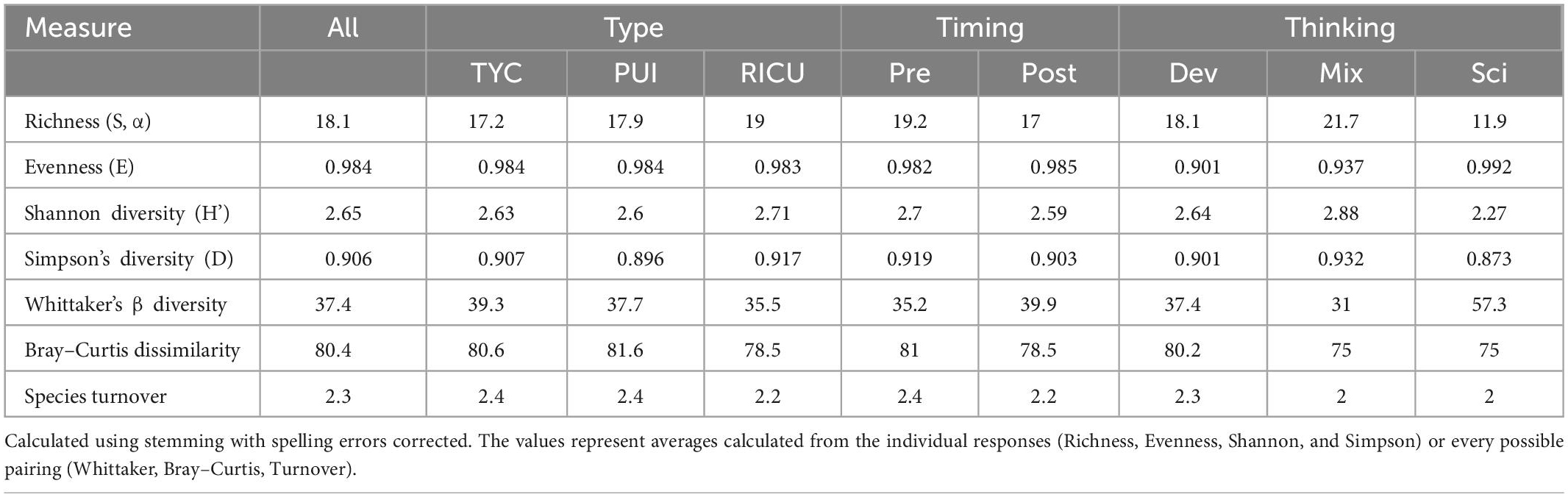
Table 3. Ecological diversity metrics.

Evenness (E) is the comparative frequency of words in a response. At an E of one, all words in a CR occur in equal frequencies, while low values mean that students heavily use certain words. The entire data set has a value of 0.98, indicating most words occur at the same frequency within an individual CRs. This is expected, as the CRs are relatively short, meaning most words are likely used once. Similar values for evenness are observed for each category within Type (range: 0.98–99; p = 0.98, ANOVA) and Timing (range: 0.98–99, p = 0.06, ANOVA). Differences in E are greatest within Thinking groups. Mixed and Developing responses have the lower values of 0.979 and 0.984, respectively, while Scientific Thinking responses have a higher value of 0.99 (p < 0.00001), with each pairing being significantly different (p < 0.05; Tukey HSD). As S is the denominator in the E formula, this change in E is likely due to the observed differences in S.

The Simpson’s index of diversity (D) is calculated using a single CR and averaged for a group. Higher numbers represent low diversity. The corpus has a value of 0.91, indicating the CRs have high diversity and are not repetitive. Type (range: 0.90–0.92; p = 0.14, ANOVA) and Timing (range 0.90–0.92; p = 0.42, ANOVA) have similar values. In contrast, within Thinking, Scientific responses have the lowest value of 0.87, while Developing and Mixed Thinking have values of 0.93 and 0.90, respectively. This difference is significant between all pairings within Thinking (p < 0.05; Tukey’s HSD). This result means there is a higher probability that two random words are the same within a Scientific CR in comparison to the other individual CRs in the Thinking categories and the corpus overall. This could, in part, be due to the Scientific category having the lowest S of the categories.

Shannon Diversity (H’) can be interpreted as the chance of predicting a random word in a CR. If a single word is very frequent in a dataset, then there is a higher likelihood a prediction will be correct (low H’). The H’ of the whole data set is 2.65. Type (range: 2.60–2.71; p = 0.34, ANOVA) and Timing (range: 2.59–2.70; p = 0.68) have similar H’ values among categories and in comparison, to the corpus as a whole. In contrast, Thinking groups have more varied H’ values of 2.88, 2.64 and 2.27 for Mixed, Developing and Scientific, respectively (p < 0.00001, ANOVA). Each pairing is significantly different within Thinking (p < 0.005, Tukey HSD). These results indicate that Scientific responses are more repetitive in comparison to other CRs. These results agree with findings using D, indicating the words in a Scientific response are more predictable. Again, this could be due to the large difference in S based within Thinking.

Whittaker’s beta (β) diversity compares the shared words between two responses. Low values represent less diversity with many shared words between the responses, while high values indicate high diversity with fewer words being shared. Our entire dataset has a β diversity of 38.6, meaning diversity within categories is much lower than diversity across all responses. When we examined β diversity within the different Types, we found slightly varied β diversities, with RICUs, PUIs, and TYCs having values of 36.7, 38.7, and 40.6, respectively. The relative similarity between the groups and the overall β diversity of the entire data set suggests there is little difference in student CRs based on Type. We found a similar result with Timing, as responses collected Pre- and Post- tutorial responses have β diversities of 37.0 and 40.4, respectively. As with the previous ED metrics, we found there is a more distinct difference in β diversity based on the groupings within Thinking. While β diversities of Developing and Mixed CRs are similar at 37.4 and 31.0, respectively, responses in the Scientific category have a much higher β diversity of 57.3. This measure supports our prediction that the largest difference would be within Thinking. These results suggest that Scientific CRs share the fewest words with each other, while Mixed CRs share the most words. We had expected that Scientific responses would share more words between responses than any other category in Thinking, as the ideas and thereby language would be the most restricted. The increased value may be due to the lower α (or S) of the Scientific CRs (9) in comparison to Mixed (21.7) and Developing (18.1) Thinking, as it is the denominator in the calculation of β.

Species turnover or half changes is calculated based on shared words between paired responses. As the number of half changes increases, responses share fewer and fewer words. We calculated species turnover for the entire data set and found the corpus has a mean of 2.3 half changes, meaning that, on average, two CRs in the corpus share less than 25% of words. We also calculated species turnover based on groupings in the categorical data. We found categories within Type, Timing, and Thinking all have similar half change ranges: Institution: 2.2–2.4 (about 21.5–19% words shared); Timing: 2.2–2.4 (about 21.5–19%), and Thinking: 2.0–2.3 (25% to about 20% words shared). Mixed and Scientific responses are the categories with the lowest values of 2.0 average half changes. These results also support our prediction that the greatest difference in text would be within Thinking. In contrast to findings using the β metric, Mixed and Scientific responses have more similar species turnover values than Developing CRs. This result agrees with our stated predictions.

A third way to examine variation is to calculate the compositional dissimilarity using a distance measure. The Bray–Curtis dissimilarity has a value of 0% when two responses are exactly the same and 100% when no words are shared between responses. We calculated this measure for each pairing in the entire corpus and found the data set has a dissimilarity of 80.36%, indicating that the text used in the entire response set is more dissimilar than similar. This indicates any CR is on average 80% different from any other, which is similar to findings from species turnover above. We also calculated the Bray–Curtis dissimilarity for the categorical groupings. Within Types, there are similar dissimilarities of 80.62, 81.57, and 78.49% for TYCs, PUIs, and RICUs, respectively. These values are also very similar to the overall data set, suggesting that each category shows similar patterns to the overall data set. For Timing, the dissimilarities are 80.94 and 78.54% for Pre- and Post-tutorial responses, respectively, suggesting there is little change in language based on Timing. In contrast, the Bray–Curtis dissimilarity of Developing responses (80.19%) is higher than that of Mixed (74.98%) or Scientific (74.94%) responses. As with species turnover, Mixed and Scientific responses have more similar values in comparison to Developing CRs.

3.3. Ordination techniques aid in visualization and reveal patterns in the corpus

Each of the measures described above describes diversity within groups or group averages of single CRs; however, we are also interested in examining and measuring potential differences between groups of CRs. Using DCA (Figure 3A) and PCoA (Supplementary Figure 2), we created two-dimensional plots of the corpus, wherein each data point is an individual CR. Points that are close to each other are more similar based on word choice and frequencies in the CR. Each axis, beginning with the x-axis, explains a descending amount of variation in the data in an additive manner and likely has multiple aspects of the data contributing to it.

FIGURE 3

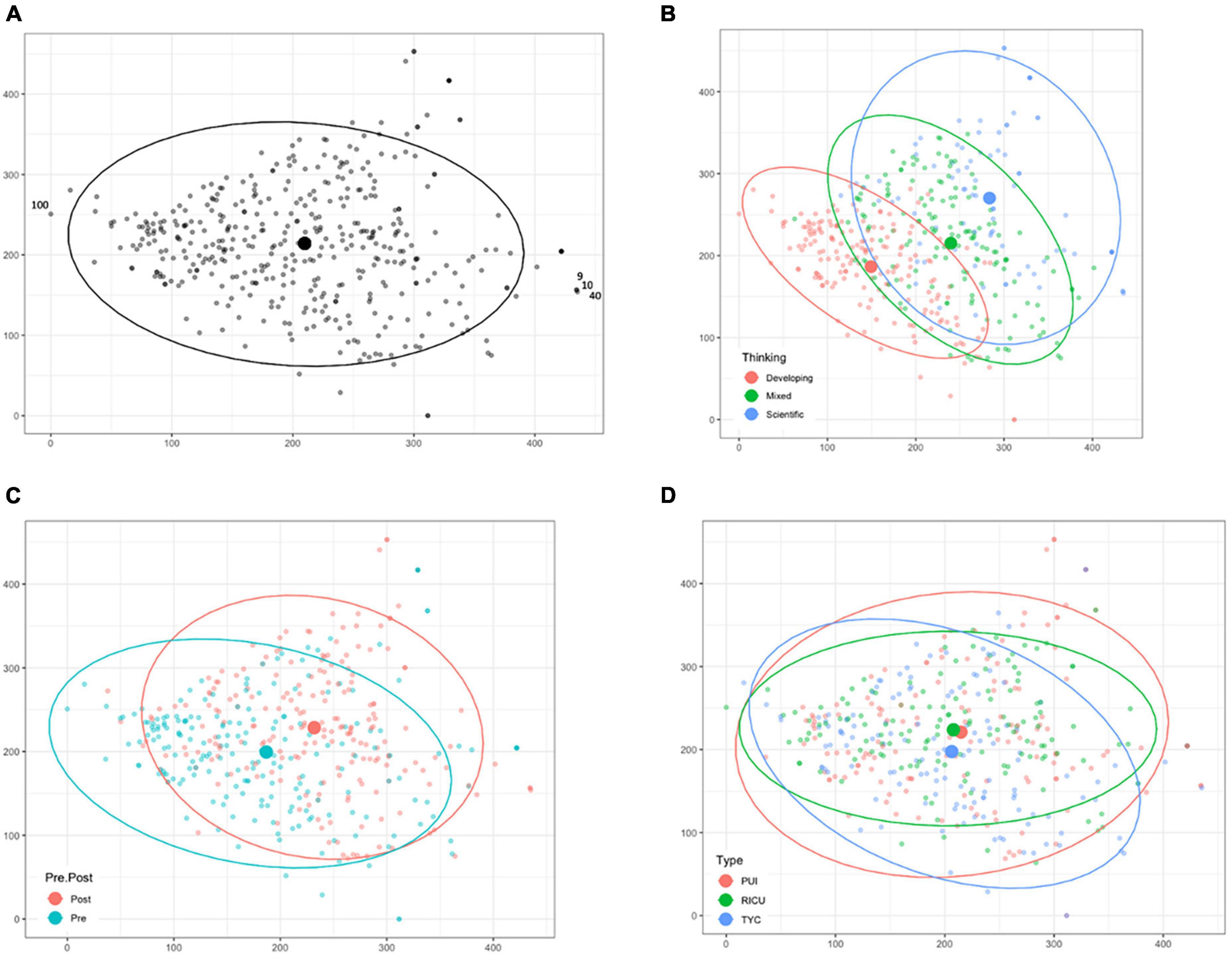
Figure 3. Detrended Correspondence Analysis (DCA). DCA was performed without any data transformation. The graphs represent 416 responses after the removal of responses 35 and 78. (A) The ordination was graphed with select responses numbered for discussion in the Results. Grouping variables including (B) Thinking, (C) Timing, and (D) Type were overlaid to compare between groups. Centroids of a given grouping variable are represented as filled circles. Ellipses are the 95% multivariate t-distribution confidence of each categorical group.

3.3.1. Detrended correspondence analysis (DCA)

DCA is uniquely suited to our purpose as the x-axis is defined exclusively as species turnover, meaning points (responses) that are the furthest away from each other on the x-axis have the highest difference in words. Additionally, every 100 units on the x-axis of the DCA graphs represents one half-change of words, allowing direct comparison of data by species turnover measure. The DCA of the entire data set results in two responses, 35 and 78, far removed from other data points. CR35 is located at (190, 5012) and reads, “Excretion.” CR78 is located at (1186, 179) and reads, “Into the air via C0₂.” (Underlined words are removed during the matrix generation process; see “Materials and methods”) These responses are very unique in comparison to other responses in the corpus (maximum axis 1 value: 449; maximum axis 2 value: 344) and render the rest of the graph uninterpretable (Supplementary Figure 3). These responses were therefore removed as outliers (McCune and Mefford, 2018) from the data set used for DCA, to better examine the remaining data. The results from the DCA explained 7.7% of the total inertia (variability) of the resulting matrix (Figure 3A). The first axis explains 4.9% of the total variability and the second axis explains 3.8%. For large data matrices, it is expected that two axes will not explain large portions of the data (Goodrich et al., 2014). To ensure the patterns are still meaningful, randomization tests determine if the axes are significant in comparison to randomized orders of the data. We found that both axes significantly explained the data (999 randomizations; p < 0.003). Data points range from 0 to 434.5 on the x-axis (Figure 3A), demonstrating that extremes of this corpus do not share any words, as 4 half changes between points is interpreted to be essentially unique.

3.3.2. Principal coordinate analysis (PCoA)

In contrast to DCA, PCoA does not have a specified, singular component or variable that is explained by any axis. As with DCA, close proximity of points means that they are more similar based on the component. We visualized our entire corpus using this ordination technique and did not observe any outlier responses that obscured the remaining data; therefore, no CRs were removed (see Supplementary Figure 2). We found six significant axes using this technique (1000 randomizations; p < 0.03). Combined, these six axes explain 36.8% of the total variance. The first axis explained 9.4% of the data, while the second explained 7.6%. We found DCA and PCoA provided similar results and will therefore only describe DCA results due to the usefulness of the first axis in calculating half-changes between responses.

3.3.3. Ordination techniques allow easy examination of corpuses of short texts

Using the ordination graph from DCA (Figure 3A), we can easily identify CRs that are very similar or different without reading the responses. Responses 9 and 10, marked in Figure 1A, are immediately next to each other and both say, “Carbon dioxide and water.” Response 40 is nearby and reads “Expelled through gas like carbon dioxide.” In contrast, data points that are on the two extreme sides of the graph share no words in common. Response 100, marked in Figure 1A, says “Probably the energy stored in the weight was used up by cells due to the decrease in calorie intake during the diet.” During an initial examination of the data, it could be useful to quickly identify CRs that are very similar or very different, especially with very large data sets that would require large amounts of time to examine individually.

3.3.4. Categorical data can be overlayed to reveal relationships among CRs

Categorical data (Thinking, Timing, and Type) associated with the CRs can be overlaid on the ordination graphs without affecting the placement of the data points, potentially illustrating patterns within the data set (Figures 3B–D). Centroids are the average coordinate value for the categorical group and are represented in the graphs by filled circles. One way to examine differences between groups is to calculate distances between group centroids. We found the largest change in position for centroids based on Thinking groups, with the total distance between the centroids being 134.2 units. Developing thinking is left-most on the x-axis at 149.3, Mixed thinking is in the middle at 241.0, and Scientific thinking is right-most at 283.5. While centroids represent the average of the group, PERMANOVAs test the relatedness of groups of data points in all dimensions using the matrix used to create the ordination graph. Within Thinking, the differences in relative distance are significant (Figure 3B; PERMANOVA; p = 0.0002; n = 88). For Timing (Figure 3C), there is slight separation of the data with post-tutorial responses as a group being more to the right of the graph. There is less distance between the two group centroids of 45 units (Pre: 186.8; Post: 231.8) in comparison to Thinking (134.2 units of separation). Using PERMANOVA, these Timing groups are also significantly different (p = 0.0002; n = 205). Finally, there appears to be minimal difference based on the Institutional Type (Figure 3D). The centroids are at most separated by only 8.4 units on the x-axis (TYC: 206.4; PUI: 214.8; RICU: 207.9), and there is not an apparent distinct clustering of the CRs. PERMANOVA reveals low statistical support for differences based on Type (p = 0.084, n = 137). While we did observe separation among groupings for Timing and Thinking, we also note the spread of responses within these individual groups is similar, which is consistent with the very similar number of half changes observed using ecological measures (Table 3).

4. Discussion

The aim of this paper was to explore the novel application of established ecological diversity measures and methods for analyzing short, explanatory texts. CR assessment offers insight into student thinking or performance through student language, but quantitative evaluation of the language diversity in CRs is limited. For this data set, we previously identified and explored patterns of ideas present in student explanations (Shiroda et al., 2021) but were dissatisfied with the available methods to quantify and represent holistic differences in language between responses and/or groups. This limitation and previous work by Jarvis (2013) comparing ecological and lexical approaches to diversity, motivated us to examine ED approaches for text analysis. Herein, ED metrics and ordination allowed us to examine student language in a different way than other methods. We were able to quantify holistic differences in language that we had observed when comparing student responses based on Thinking, Timing, and Type. The purpose of the current work is meant to be confirmatory in nature, in that we have already explored this CR corpus in previous work and had expected results based on this previous qualitative work. Namely, we expected the greatest difference in language to be among Thinking, some difference based on Timing, and little difference based on Type. Using these predictions, we could examine whether the outcomes from the ED metrics and ordination techniques corresponded to construct-relevant differences in student CRs.

Overall, we applied seven ED measures to this data set. Richness or alpha diversity, while helpful in other calculations, does not reveal anything uniquely useful, as this can be easily calculated with other forms of text analysis. Similarly, evenness was not particularly useful in itself given how short most responses were, as students are unlikely to heavily repeat a given word in only one to three sentences. However, this information is important for interpretation of the other metrics and could be more useful in longer texts than ones used here. Shannon and Simpson diversity metrics are similar to existing lexical diversity measures in that they examine diversity of individual responses. One advantage of these ecological measures in comparison to those in lexical diversity is that they have no established lower limit on length. In spite of this, Shannon and Simpson are still influenced by evenness and richness. While this may not be problematic for all CR corpora, our data set had differences in richness based on Thinking and Timing, making the Shannon and Simpson measures more difficult to interpret for those categories of CRs.

We found comparing pairs of responses using Whittaker’s β, Bray–Curtis Dissimilarity, and Species Turnover to be the most interesting expansion of current text analysis approaches for our applications. These three measures each quantify differences between responses in slightly different ways. Additionally, each identified similar patterns in the categorical data, which correspond well to our previous, qualitative analysis of the corpus. Namely, that grouping responses by Thinking category has the largest effect on all three measures and suggesting that differences in student texts exist between sub-groups. Additionally, all three measures found that Developing CRs are very similar to the entire corpus. For each measure, Developing and Scientific responses are consistently most different from each other; however, Mixed responses are more similar to Developing responses with Whittaker’s β, but more similar to Scientific responses when measured by Bray–Curtis Dissimilarity and Species Turnover. This result could be due to the difference in Richness (alpha) based on Thinking. Bray–Curtis Dissimilarity and Species Turnover also more closely agreed with our prediction that Mixed Thinking CRs would be more similar to Scientific CRs than Developing ones. We also identified a general pattern in the corpus that Scientific responses are more similar to themselves than the corpus overall. This is the only category within Type, Thinking, or Timing that consistently had a unique value. This supports observations from rubric development and human coding during qualitative analysis, in that there are generally fewer ways to write correctly about a scientific idea than ways to write about incorrect or other, non-scientific ideas (Sripathi et al., 2019; Shiroda et al., 2021). We are excited these quantitative measures support these qualitative observations and consider these metrics promising for critically testing student language. As Whittaker’s β shows a different pattern than Bray–Curtis Dissimilarity and Species Turnover, we considered which measures best suit our purposes. Bray–Curtis Dissimilarity and Species Turnover are less sensitive to differences in richness, which we prioritize because this difference is already apparent in the richness measure itself. Additionally, Whittaker’s β is generally considered to be a very simple representation of diversity, which also contributes to our preference for Bray–Curtis Dissimilarity and Species Turnover.

Ordination offers a unique visualization of the CR corpus and greatly assists our comparison of language among different groupings of the CR corpus. While we can and did qualitatively examine the responses previously during human thematic coding (Sripathi et al., 2019; Shiroda et al., 2021), these processes take time. We imagine these techniques could be helpful as an exploratory phase of CR analysis, similar to LSA, to look for unique responses or determine if there are potential language differences among groups. Here, we used ordination in a confirmatory fashion. We expected Thinking to most affect student language because that is how the rubric and coding were designed. Similarly, we were expecting there to be differences based on Timing since changes in Thinking are associated with Timing (Uhl et al., 2021). In contrast, Shiroda et al. (2021) found fewer apparent differences based on the institutional Type. These expectations are further supported by text analysis through having a decreasing number of predictive words. Indeed, ordination analysis reflected these expectations (Figures 3B–D), both in the more distinct clustering of responses using the categorical data and in the distance between group centroids. These overall clustering patterns could be observed in both DCA (Figures 3B–D) and in PCoA (Supplementary Figures 2B–D). While observing these patterns and calculating the half changes in the DCA are useful, PERMANOVA tests are a promising method to quantitatively compare groups of responses. Using this test, we confirm the largest difference in student text is among the groups within Thinking and between Timing, while there is limited support for differences in text among the Institutional Types groups. This allows us to conclude that student word choice differs for sub-groups in both Thinking and Timing, while word choice for CRs to this question is not related to Institutional Type. Differences between Thinking are heavily supported by the rubric, but the lack of differences in language among the institutional Types was only qualitatively supported in Shiroda et al. (2021). In contrast, these PERMANOVA tests provide direct statistical rigor to the observations that are not possible with other analyses. These methods could be particularly useful in comparing differential language between groups to better understand the different ways students convey understanding. For example, when originally working with this data set, we were attempting to examine performance differences for a computerized text classification model with this data set in comparison to one that was used to create the model (Shiroda et al., 2021). Using these ordination techniques, one would be able to quickly and visually compare the original and new data sets to determine if student language was different between the sets. We have since successfully applied ordination techniques to understand other computer scoring model performance (Shiroda et al., in review¹). In comparison, similar text analysis approaches such as LSA may be helpful in exploratory analyses to find prevalent themes in responses but would be less helpful for this goal as they do not reveal differences in specific words and instead condense the meaning of the language. As such our novel application of ecological diversity measures may be used in complementary fashion with other text analysis methods depending on the research study.

We performed quantitative text analysis to support our expectations for the differences in CRs among the categorical data. Indeed, we found that these differences in ED measures correspond to differences in words identified by text analysis and can be further linked to differences observed in human-assigned ideas (i.e., student thinking). This helps validate the ED metrics by identifying words and phrases which differ significantly in their usage between sub-groups. However, the ED methods and text analysis provide different pieces of information. While ED methods help compare individual CRs to each other, text analysis helps us understand differences in the actual text identified using the ED methods. For example, the words that are differentially used in responses categorized by coders as Scientific ideas include H₂O, water, releas-, cellular, respir- and form. Most of these words are closely linked to the Scientific ideas identified in the coding rubric categories of Correct Products and Exhalation. The words CO₂, carbon, respir-, convert, and dioxid- were more common in both Mixed and Scientific responses, indicating considerable overlap in how students describe how carbon leaves the system. As water was only frequently used in Scientific thinking, this analysis suggests students with Mixed thinking still struggle with how water leaves the body during weight loss. This information would not be clear using only the ecological methods we describe here. We therefore suggest that ecological methods be used in conjunction with text analysis to examine CR corpora.

In summary, we found that ED measures can be usefully applied to text analysis of students’ short text explanations. In particular, methods that analyze between response variation (Whittaker’s β, Bray–Curtis Dissimilarity, Species Turnover, and ordination) were most useful for our interests in understanding CRs based on categorical data. For other research interests, Simpson, or Shannon diversity measures may be more informative. Similarly, richness and evenness do not seem to provide much additional insight to text diversity with this data set but are needed to better interpret the other ED measures and could be more informative for longer texts.

4.1. Future directions and considerations for additional applications

These techniques help reveal differences in diversity within student language and different categories of the corpus; however, further analysis is needed to understand these results. With the exception of the first axis of DCA, it is difficult to interpret ordinations for specific differences in the text, as each axis represents multiple factors in the data. Similarly, while the different metrics (E, S, D, H’, β, Bray–Curtis Dissimilarity and species turnover) quantify diversity and provide markers for the amount of variety in a group of responses, the metrics do not specify the nature of the differences. Determining these differences in language within the text is better achieved by text analysis, along with traditional qualitative techniques, such as coding of the responses. Therefore, we recommend that ED and ordination analysis be done to supplement text analysis and qualitative methods. For example, we performed text analysis as a proxy to differences in word choice, but examining the predictive words reveals an important difference in language. Water is only increased in Scientific CRs while sweat and urine are increased in Mixed thinking. This indicates that students with Mixed thinking are still having trouble articulating how water leaves the body in relation to weight loss and could serve as a target for improving student explanations. If we had only applied the ecological methods, we would know that there is a difference but not have an actionable conclusion that could promote teaching and learning.

We consider these analyses broadly applicable to any corpus of short texts. Our group has already successfully applied these analyses to multiple CR corpora to examine the progression of student language across physiology contexts (Shiroda et al., in review²) and explore the effect of overlapping language on the success of machine learning models for automated assessment [Shiroda et al., in review (see text footnote 1)]. As with any ecological study, we began this study by considering the nature of our data set and recommend this as a critical first step before applying these methods to new data sets. We note that in applying these diversity methods to our data set, we made purposeful decisions about text processing, many of which led to meaningful interpretation of the results. However, we do not consider these decisions absolute for all applications and acknowledge that other data sets and/or outcomes will most likely justify different text processing decisions. For example, we chose to stem words for the diversity metrics, but not remove any other words. We chose these settings as it most closely matches the text analysis protocols that were used in the previous work. While we found the text processing method did not affect the overall patterns we found, this may not be true for other data sets (Supplementary Table 2). We selected this method as the settings are most similar to previous work, allowing this work to be more directly compared to previous work. For some CRs, the distinction between stemming and lemmatization may be important. For example, stemming is not exact in removing tense. It will remove words that maintain the same root but do not collapse the form of words that change fully such as “to be.” Since our question was in past tense, there was not a large number of differences in tense; however, for other data sets ensuring tense is collapsed may be more important to reveal patterns. Lemmatization does make these changes, but also collapses comparative words. For example, great, greater, and greatest are collapsed. Depending on the context, maintaining the levels of comparison could differentiate student thinking and be important to maintain. We strongly suggest that text processing decisions should be purposeful and tailored to the corpus.

Ordination requires separate, equally purposeful decisions to function correctly. We removed less meaningful words (e.g., articles, conjunctions, propositions), as common, unmeaningful words can skew the overall pattern of the data set. However, it is important to keep the CR context in mind when choosing text processing strategies. For example, if students are explaining the process of diffusion as part of a science course, the words “in” and “out” would be critical to student meaning in that context and should not be removed. We advise others using these techniques to examine their data to determine whether certain prepositions or words may be important. While text processing steps will likely differ, DCA and PCoA are likely to be most useful to examine language diversity in most CR data sets. A key advantage of these two approaches is that these methods can handle data sets with high percentages of zeros, which is likely to occur in most lexical datasets (i.e., short, content-rich texts). However, other ordination methods should be considered during the initial phases of data analysis to make sure the approach is appropriate for the data set and these other ordination methods explored further. For example, if a set of CRs is highly redundant, this could result in a lower percentage of zeros, opening the possibility of using ordination methods that our data excluded. We recommend that researchers who wish to apply these methods, but do not have an ecology background, seek out helpful texts including Peck (2010) and Palmer (2019), and a website maintained by Oklahoma State University: http://ordination.okstate.edu/key.htm. We view the versatility and the ability to make purposeful choices for each data as a strength of the methodology.

While this study was confirmatory and the current paper is intended to describe the approach, we believe these techniques can also be used in an exploratory fashion. We were originally motivated to perform this work because we were excited by the potential to expand quantitative approaches to language diversity in CRs (or short blocks of text). The data visualization, various metrics, and statistical computations of our ED methods offer a rich and wide range of results that bring statistical and quantitative methods to a field that typically relies on qualitative methods. Overall, these ED techniques provide quantitative methods that will allow researchers to examine short texts in a novel way in comparison to current text analysis methods. Within STEM education research, these techniques can assist in the examination of differences in student writing and ideas over time, effects of a pedagogical intervention, differences in explanations across contexts for cross-cutting concepts, and many other forms of categorical data.

Data availability statement

The raw word matrix, curated matrix used for ordination, and associated categorical data are available on GitHub.1 researchers who are interested in the responses may contact the KH, haudekke@msu.edu.

Ethics statement

The studies involving human participants were reviewed and approved by the Michigan State University (x10–577). Written informed consent for participation was not required for this study in accordance with the national legislation and the institutional requirements.

Author contributions

MS performed the data analysis and primarily drafted the manuscript. MF assisted the data analysis and drafted the manuscript. KH provided the feedback on the data analysis and manuscript. All authors were involved in project design, execution, and editing of the manuscript.

Funding

This material was based upon work supported by the National Science Foundation under Grant Nos. 1323162 and 1660643.

Acknowledgments

We would like to thank Marisol Mercado Santiago for her work on reviewing lexical diversity and Ryan Terrill for his expertise in R. We would also like to thank Juli Uhl, Leonora Kaldaras, and Jennifer Kaplan for helpful edits and Brian Nohomovich for discussions throughout the project.

Conflict of interest

The authors declare that the research was conducted in the absence of any commercial or financial relationships that could be construed as a potential conflict of interest.

Publisher’s note

All claims expressed in this article are solely those of the authors and do not necessarily represent those of their affiliated organizations, or those of the publisher, the editors and the reviewers. Any product that may be evaluated in this article, or claim that may be made by its manufacturer, is not guaranteed or endorsed by the publisher.

Supplementary material

The Supplementary Material for this article can be found online at: https://www.frontiersin.org/articles/10.3389/feduc.2023.989836/full#supplementary-material

Footnotes

1. ^ Shiroda, M., Doherty, J. H., and Haudek, K. C. (in review). Exploring attributes of successful machine learning assessments for scoring of undergraduate constructed responses assessment items. Uses of artificial intelligence in STEM education. Oxford: Oxford University Press.
2. ^ Shiroda, M., Doherty, J. H., Scott, E. E., and Haudek, K. C. (in review). Covariational reasoning and item context affect language in undergraduate mass balance written explanations. Adv. Physiol. Educ.

References

American Association for the Advancement of Science (2011). Vision and change in undergraduate biology education: a view for the 21st century. Available online at: https://live-visionandchange.pantheonsite.io/wp-content/uploads/2011/03/Revised-Vision-and-Change-Final-Report.pdf [accessed August 18, 2021].

Google Scholar

Anderson, M. J. (2017). “Permutational multivariate analysis of variance (PERMANOVA),” in Wiley StatsRef: statistics reference online, eds N. Balakrishnan, T. Colton, B. Everitt, W. Piegorsch, F. Ruggeri, and J. L. Teugels (Hoboken, NJ: Wiley), doi: 10.1002/9781118445112.stat07841

CrossRef Full Text | Google Scholar

Birenbaum, M., Tatsuoka, K. K., and Gutvirtz, Y. (1992). Effects of response format on diagnostic assessment of scholastic achievement. Appl. Psychol. Meas. 16, 353–363. doi: 10.1177/014662169201600406

CrossRef Full Text | Google Scholar

Borges, V. R. P., Esteves, S., de Nardi Araujo, P., de Oliveira, L. C., and Holanda, M. (2018). “Using principal component analysis to support students’ performance prediction and data analysis,” in Proceedings of the Brazilian symposium on computers in education, Vol. 29, 1383. doi: 10.5753/cbie.sbie.2018.1383

CrossRef Full Text | Google Scholar

Boumans, J. W., and Trilling, D. (2016). Taking stock of the toolkit: An overview of relevant automated content analysis approaches and techniques for digital journalism scholars. Digital J. 4, 8–23. doi: 10.1080/21670811.2015.1096598

CrossRef Full Text | Google Scholar

Bray, J. R., and Curtis, J. T. (1957). An ordination of upland forest communities of southern Wisconsin. Ecol. Monogr. 27, 325–349. doi: 10.2307/1942268

CrossRef Full Text | Google Scholar

Choi, W., and Jeong, H. (2016). Finding an appropriate lexical diversity measurement for a small-sized corpus and its application to a comparative study of L2 learners’ writings. Multimed. Tools Appl. 75, 13015–13022. doi: 10.1007/s11042-015-2529-1

CrossRef Full Text | Google Scholar

Covington, M. A., and McFall, J. D. (2010). Cutting the gordian knot: the moving-average type–token ratio (MATTR). J. Quant. Linguisti. 17, 94–100. doi: 10.1080/09296171003643098

CrossRef Full Text | Google Scholar

Deerwester, S. C., Dumais, S. T., Landauer, T. K., Furnas, G. W., and Harshman, R. A. (1990). Indexing by latent semantic analysis. J. Am. Soc. Inf. Sci. 41, 391–407. doi: 10.1002/(SICI)1097-4571(199009)41:6<391::AID-ASI1>3.0.CO;2-9

CrossRef Full Text | Google Scholar

Gauch, H. G. (1982). Noise reduction by eigenvector ordinations. Ecology 63, 1643–1649. doi: 10.2307/1940105

CrossRef Full Text | Google Scholar

Gerard, L. F., and Linn, M. C. (2016). Using automated scores of student essays to support teacher guidance in classroom inquiry. J. Sci. Teacher Educ. 27, 111–129. doi: 10.1007/s10972-016-9455-6

CrossRef Full Text | Google Scholar

Gibbs, G. R. (2007). Thematic coding and categorizing. Analyzing qualitative data. London: SAGE Publications, Ltd.

Google Scholar

Goodrich, J. K., Di Rienzi, S. C., Poole, A. C., Koren, O., Walters, W. A., Caporaso, J. G., et al. (2014). Conducting a microbiome study. Cell 158, 250–262. doi: 10.1016/j.cell.2014.06.037

PubMed Abstract | CrossRef Full Text | Google Scholar

Graesser, A. C., McNamara, D. S., and Kulikowich, J. M. (2011). Coh-Metrix: Providing multilevel analyses of text characteristics. Educ. Res. 40, 223–234. doi: 10.3102/0013189X11413260

CrossRef Full Text | Google Scholar

Haudek, K. C., Prevost, L. B., Moscarella, R. A., Merrill, J., and Urban-Lurain, M. (2012). What are they thinking? Automated analysis of student writing about acid–base chemistry in introductory biology. CBE Life Sci. Educ. 11, 283–293. doi: 10.1187/cbe.11-08-0084

PubMed Abstract | CrossRef Full Text | Google Scholar

IBM Corp (2020). IBM SPSS statistics for windows (Version 27.0) [computer software]. Armonk, NY: IBM Corp.

Google Scholar

Jarvis, S. (2013). Capturing the diversity in lexical diversity. Lang. Learn. 63, 83–106. doi: 10.1111/j.1467-9922.2012.00739.x

CrossRef Full Text | Google Scholar

Jescovitch, L. N., Scott, E. E., Cerchiara, J. A., Merrill, J., Urban-Lurain, M., Doherty, J. H., et al. (2021). Comparison of machine learning performance using analytic and holistic coding approaches across constructed response assessments aligned to a science learning progression. J. Sci. Educ. Technol. 30, 150–167. doi: 10.1007/s10956-020-09858-0

CrossRef Full Text | Google Scholar

Jost, L. (2006). Entropy and diversity. OIKOS 113, 363–375. doi: 10.1111/j.2006.0030-1299.14714.x

CrossRef Full Text | Google Scholar

Jurasinski, G., Retzer, V., and Beierkuhnlein, C. (2009). Inventory, differentiation, and proportional diversity: a consistent terminology for quantifying species diversity. Oecologia 159, 15–26. doi: 10.1007/s00442-008-1190-z

PubMed Abstract | CrossRef Full Text | Google Scholar

Kaplan, J. J., Haudek, K. C., Ha, M., Rogness, N., and Fisher, D. G. (2014). Using lexical analysis software to assess student writing in statistics. Technol. Innov. Stat. Educ. 8. doi: 10.5070/T581020235

CrossRef Full Text | Google Scholar

Koizumi, R. (2012). Relationships between text length and lexical diversity measures: Can we use short texts of less than 100 tokens? Vocab. Learn. Instr. 1, 60–69. doi: 10.7820/vli.v01.1.koizumi

CrossRef Full Text | Google Scholar

Krajcik, J. S. (2021). Commentary—Applying machine learning in science assessment: Opportunity and challenges. J. Sci. Educ. Technol. 30, 313–318.

Google Scholar

Landauer, T. K., and Psotka, J. (2000). Simulating Text Understanding for Educational Applications with Latent Semantic Analysis: Introduction to LSA. Interact. Learn. Environ. 8, 73–86. doi: 10.1076/1049-4820(200008)8:2;1-B;FT073

CrossRef Full Text | Google Scholar

Lande, R. (1996). Statistics and partitioning of species diversity, and similarity among multiple communities. Oikos 76, 5–13. doi: 10.2307/3545743

CrossRef Full Text | Google Scholar

LaVoie, N., Parker, J., Legree, P. J., Ardison, S., and Kilcullen, R. N. (2020). Using latent semantic analysis to score short answer constructed responses: automated scoring of the consequences test. Educ. Psychol. Meas. 80, 399–414. doi: 10.1177/0013164419860575

PubMed Abstract | CrossRef Full Text | Google Scholar

Malvern, D., Richards, B., Chipere, N., and Durán, P. (2004). Lexical diversity and language development. Berlin: Springer. doi: 10.1057/9780230511804

CrossRef Full Text | Google Scholar

McCune, B., and Mefford, M. J. (2018). PC-ORD. Multivariate analysis of ecological data. Version 7.08.

Google Scholar

McMurdie, P. J., and Holmes, S. (2013). phyloseq: an R package for reproducible interactive analysis and graphics of microbiome census data. PLoS One 8:e61217. doi: 10.1371/journal.pone.0061217

PubMed Abstract | CrossRef Full Text | Google Scholar

Nehm, R. H., and Reilly, L. (2007). Biology majors’ knowledge and misconceptions of natural selection. BioScience 57, 263–272. doi: 10.1641/B570311

CrossRef Full Text | Google Scholar

Nehm, R. H., and Schonfeld, I. S. (2008). Measuring knowledge of natural selection: a comparison of the CINS, an open response instrument, and an oral interview. J. Res. Sci. Teach. 45, 1131–1160. doi: 10.1002/tea.20251

CrossRef Full Text | Google Scholar

Ngss Lead States (2013). Next generation science standards; for states, by states; 2013. Available online at: https://www.nextgenscience.org/ (accessed January 5, 2022).

Google Scholar

Noyes, K., McKay, R. L., Neumann, M., Haudek, K. C., and Cooper, M. M. (2020). Developing computer resources to automate analysis of students’ explanations of London dispersion forces. J. Chem. Educ. 97, 3923–3936. doi: 10.1021/acs.jchemed.0c00445

CrossRef Full Text | Google Scholar

Palmer, M. (n.d.). Ordination methods for ecologists. The ordination web page. Available online at: http://ordination.okstate.edu/

Google Scholar

Palmer, M. W. (2019). “Gradient analysis of ecological communities (ordination),” in Handbook of environmental and ecological statistics, eds A. Gelfand, M. Fuentes, P. Hoeting, and R. L. Smith (Boca Raton: CRC Press), 241–274. doi: 10.1201/9781315152509-12

CrossRef Full Text | Google Scholar

Peck, J. E. (2010). Multivariate analysis for community ecologists: step-by-step using PC-ORD. Gleneden Beach, OR: MjM Software Design, 162.

Google Scholar

Rajaraman, A., and Ullman, J. (2011). Mining of massive datasets. Cambridge: Cambridge University Press. doi: 10.1017/CBO9781139058452

CrossRef Full Text | Google Scholar

Roswell, M., Dushoff, J., and Winfree, R. (2021). A conceptual guide to measuring species diversity. Oikos 130, 321–338. doi: 10.1111/oik.07202

CrossRef Full Text | Google Scholar

Scott, E. E., Cerchiara, J., McFarland, J. L., Wenderoth, M. P., and Doherty, J. H. (2022). How students reason about matter flows and accumulations in complex biological phenomena: an emerging learning progression for mass balance. J. Res. Sci. Teach. 60, 63–99. doi: 10.1002/tea.21791

CrossRef Full Text | Google Scholar

Shannon, C. E. (1948). A mathematical theory of communication. Bell Syst. Tech. J. 27, 623–656. doi: 10.1002/j.1538-7305.1948.tb00917.x

CrossRef Full Text | Google Scholar

Shiroda, M., Uhl, J. D., Urban-Lurain, M., and Haudek, K. C. (2021). Comparison of computer scoring model performance for short text responses across undergraduate institutional types. J. Sci. Educ. Technol. 31, 117–128. doi: 10.1007/s10956-021-09935-y

CrossRef Full Text | Google Scholar

Si, F. J. (2006). The application of principal component analysis in teaching evaluation. Intelligence 26, 78–79.

Google Scholar

Simpson, E. H. (1949). Measurement of diversity. Nature 163:688. doi: 10.1038/163688a0

CrossRef Full Text | Google Scholar

Sripathi, K. N., Moscarella, R. A., Yoho, R., You, H. S., Urban-Lurain, M., Merrill, J., et al. (2019). Mixed student ideas about mechanisms of human weight loss. CBE Life Sci. Educ. 18:ar37. doi: 10.1187/cbe.18-11-0227

PubMed Abstract | CrossRef Full Text | Google Scholar

Syms, C. (2008). “Ordination’,” in Encyclopedia of ecology, eds S. E. Jørgensen and B. D. Fath (Amsterdam: Elsevier), 2572–2581. doi: 10.1016/B978-008045405-4.00524-3

CrossRef Full Text | Google Scholar

Tuomisto, H. (2010). A diversity of beta diversities: straightening up a concept gone awry. Part 2. Quantifying beta diversity and related phenomena. Ecography 33, 23–45. doi: 10.1111/j.1600-0587.2009.06148.x

CrossRef Full Text | Google Scholar

Tweedie, F. J., and Baayen, R. H. (1998). How variable may a constant be? Measures of lexical richness in perspective. Comput. Hum. 32, 323–352. doi: 10.1023/A:1001749303137

CrossRef Full Text | Google Scholar

Uhl, J. D., Shiroda, M., and Haudek, K. C. (2022). Developing assessments to elicit and characterize undergraduate mechanistic explanations about information flow in biology. J. Biol. Educ. 1–20. doi: 10.1080/00219266.2022.2041460

CrossRef Full Text | Google Scholar

Uhl, J. D., Sripathi, K. N., Meir, E., Merrill, J., Urban-Lurain, M., and Haudek, K. C. (2021). Automated writing assessments measure undergraduate learning after completion of a computer-based cellular respiration tutorial. CBE Life Sci. Educ. 20:ar33. doi: 10.1187/cbe.20-06-0122

PubMed Abstract | CrossRef Full Text | Google Scholar

Vellend, M. (2001). Do commonly used indices of β-diversity measure species turnover? J. Veg. Sci. 12, 545–552. doi: 10.2307/3237006

CrossRef Full Text | Google Scholar

Voleti, R., Liss, J. M., and Berisha, V. (2020). A review of automated speech and language features for assessment of cognitive and thought disorders. IEEE J. Sel. Top. Signal Process. 14, 282–298. doi: 10.1109/JSTSP.2019.2952087

PubMed Abstract | CrossRef Full Text | Google Scholar

Welbers, K., Van Atteveldt, W., and Benoit, K. (2017). Text analysis in R. Commun. Methods Meas. 11, 245–265. doi: 10.1080/19312458.2017.1387238

CrossRef Full Text | Google Scholar

Whittaker, R. H. (1967). Gradient analysis of vegetation. Biol. Rev. 42, 207–264. doi: 10.1111/j.1469-185X.1967.tb01419.x

PubMed Abstract | CrossRef Full Text | Google Scholar

Whittaker, R. H. (1969). Evolution of diversity in plant communities. Brookhaven Symp. Biol. 22, 178–195.

Google Scholar

Whittaker, R. H. (1972). Evolution and measurement of species diversity. Taxon 21, 213–251. doi: 10.2307/1218190

CrossRef Full Text | Google Scholar

Xian, S., Xia, H., Yin, Y., Zhai, Z., and Shang, Y. (2016). Principal component clustering approach to teaching quality discriminant analysis. Cogent Educ. 3:1194553. doi: 10.1080/2331186X.2016.1194553

CrossRef Full Text | Google Scholar

Yuan, Y., Buckland, S. T., Harrison, P. J., Foss, S., and Johnston, A. (2016). Using species proportions to quantify turnover in biodiversity. JABES 21, 363–381. doi: 10.1007/s13253-015-0243-0

CrossRef Full Text | Google Scholar

Zelený, D. (2021). Analysis of community ecology data in R. Available online at: https://www.davidzeleny.net/anadat-r/doku.php/en:div-ind (accessed June 26, 2022).

Google Scholar

Zenker, F., and Kyle, K. (2021). Investigating minimum text lengths for lexical diversity indices. Assess. Writ. 47:100505. doi: 10.1016/j.asw.2020.100505

CrossRef Full Text | Google Scholar

Zhai, X., Haudek, K. C., and Ma, W. (2022). Assessing argumentation using machine learning and cognitive diagnostic modeling. Res. Sci. Educ. doi: 10.1007/s11165-022-10062-w

CrossRef Full Text | Google Scholar