The dynamics of lowland river sections of Danube and Tisza in the Carpathian basin

The paper presents a detailed statistical analysis of data from 41 hydrometric stations along the Danube (section in the Carpathian Basin) and its longest tributary, the Tisza River. Most records cover 2–3 decades with an automated high temporal sampling frequency (15 min), and a few span 120 years with daily or half-daily records. The temporal sampling is not even and exhibits strong irregularities. The paper demonstrates that cubic spline fits and down-sampling (where necessary) produce reliable, evenly sampled time series that smoothly reconstruct water level and river discharge data. Almost all the water level and discharge records indicate a decadal decreasing trend for annual maximum values. The timing (day of the year) for annual maxima and minima is evaluated. While minimum values do not show coherent tendencies, annual maxima exhibit increasing trends for the Tisza but decreasing trends for the Danube (earlier onset). Various possibilities for the explanations of these observations are listed. The empirical histograms for half-daily water level changes can be well-fitted by piecewise-exponential functions containing four or three sections, consistent with the understanding that level changes are deterministic rather than stochastic processes, as is well known in hydrology. Such statistical tests can serve as benchmarks for modeling water levels and discharges. Extracted periods by the Lomb-Scargle algorithm (suitable for unevenly sampled time series) and the long-time means indicate the expected annual seasonality. Resampled time series (1-hour frequency) were evaluated by standard Fourier and Welch procedures, revealing some secondary peaks in the spectra indicating quasi-periodic components in the signals. Further significance tests are in progress, along with attempts at explanations. Secondary peaks may indicate environmental changes, the future investigation of which could reveal important correlations.

1 Introduction

Water level and discharge are crucial hydrological variables that provide insights into the state of a river system and its response to various factors (Rhoads, 2020a; Fekete et al., 2021; Bárdossy and El Hachem, 2021). Water levels and discharge are mainly influenced by meteorological, landscape, and climatic forcing, but changes in landscape management in the catchment area also significantly impact floods (Clark, 1987).¹ Time series analysis of these variables is essential to understand their behavior and identify potential patterns and trends (Ghil et al., 2002; Bogárdi and Fekete, 2021; Fekete et al., 2021). One commonly employed method in this regard is the examination of climatic means, which helps establish a baseline for comparison and assess deviations from typical conditions. Power spectrum analysis is another valuable tool used to identify periodicities and dominant frequencies in the time series data, shedding light on potential natural cycles or recurring patterns. Additionally, trends in annual maxima and minima of river water level and discharge are of particular interest as they reveal changes in extreme events, such as floods and droughts, which can have significant impacts on both the environment and human activities. Understanding the timing of these annual maxima and minima is equally essential, as it may indicate shifts in seasonal patterns and potential alterations in precipitation patterns or snowmelt regimes (Bertola et al., 2020; Kemter et al., 2020). Such information is valuable for water resource management, flood forecasting, and ecosystem preservation.

The further structure of this section is as follows. The background to the present research will be briefly presented, highlighting in what sense and in what respects the key findings of this study can be considered as results that have not been previously presented or not in sufficient detail. Additionally, the contribution of these results to the understanding of river properties, both in absolute terms and in relation to other disciplines such as climate change, will be discussed. Then, the environmental factors that significantly impact water level and water discharge are briefly described, followed by an introduction to the research methods, tools, and directions that have been developed in the field of river discharge and water level research.

Flood events primarily originate from meteorological conditions, especially precipitation or snow melt. As global changes progress, alterations in precipitation patterns can significantly impact the types of floods that occur (Blöschl et al., 2017; Blöschl et al., 2019; Kemter et al., 2023; Tarasova et al., 2023). Clausius-Clapeyron scaling suggests that extreme precipitation intensities increase in hourly or shorter durations by approximately 6.5% per $1°$C atmospheric warming as the water holding capacity increases (Guerreiro et al., 2018; Vergara-Temprado et al., 2021). Observations reveal very high regional variability, albeit with an apparent increasing tendency in most continents (Guerreiro et al., 2018; Vergara-Temprado et al., 2021; Ayat et al., 2022; Li et al., 2022; Kendon and Short, 2023).

Landscapes play a vital role in the water cycle and the intricate journey of water. They receive water through precipitation and subsequently engage in a dynamic process of transporting, storing, mixing, and releasing it. This movement occurs in two directions: downward, feeding streams, and upward, nourishing vegetation. How landscapes manage these processes significantly impacts various natural phenomena, including floods and droughts, biogeochemical cycles, the transportation of contaminants, and the overall health of terrestrial and aquatic ecosystems. Understanding these complex interactions can be challenging as many crucial processes occur out of sight, deep within the subsurface (Beven, 2011; Kirchner et al., 2023).

Among the long-term consequences of climate change, the impact on water yields and flows in rivers is very important, as most of the population lives near rivers and very often rivers are used as drinking water sources, but also for agriculture, either for water cycling as natural or for irrigation as artificial water supply. As has already been shown by comparing several climate models, adverse impacts are expected in several of the Earth’s major river basins based on climate change models (van Vliet et al., 2013). The study found that both the Danube and the Tisza river basins are affected by changes in the direction of the change, especially in case of low flows, (see their Figure 3). In the following, the paper briefly describes some of the research methods widely applied to long term studies of water yields and water levels. These are hydrological models, statistical methods and most recently the use of AI for analysis.

Hydrological models are recognized as essential tools for managing water and environmental resources (Ponce and Hawkins, 1996; Beven, 2011; Devia et al., 2015; Jehanzaib et al., 2022; Kirchner et al., 2023). Traditional runoff models can be classified into three main categories: empirical, conceptual, and physically based models. Empirical methods for estimating direct runoff from rainfall are well established in hydrological engineering and environmental impact analyses. The popularity is rooted in their convenience, simplicity, and responsiveness to four easily grasped catchment properties: soil type, land use, surface condition, and antecedent condition (Ponce and Hawkins, 1996; Laizé and Hannah, 2010; Beven, 2011; Devia et al., 2015; Jehanzaib et al., 2022; Kirchner et al., 2023). Conceptual (or parametric) models describe several components of hydrological sub-processes. They consist of numerous interconnected reservoirs which represent the physical elements in a catchment. They are recharged by rainfall, and infiltration, and are emptied by evaporation, runoff, drainage, etc. Semi-empirical equations are used in such methods, and the model parameters are assessed not only from field data but also through calibration. A large number of meteorological and hydrological records are required for calibration. For this reason, parametric models cannot be applied everywhere (Hrachowitz et al., 2013; Yang et al., 2019; Jehanzaib et al., 2022; Kirchner et al., 2023). There are also parametric water level and runoff models however, the results of which are already explanatory of the climate change phenomena (Booij, 2005). A physical process-based runoff model refers to a collection of differential equations (both in space and time) utilized to estimate the amount of runoff based on various parameters describing the characteristics of a watershed (Devia et al., 2015; Jehanzaib et al., 2022). These models require two crucial inputs: rainfall data and drainage area. Additionally, they take into account watershed features such as soil properties, vegetation cover, watershed topography, soil moisture content, evaporation, evapotranspiration, and groundwater aquifer characteristics.

There are many statistical methods for time series analysis, most of them available as pre-written routines in many programming environments, including in the SciPy library in Python. In the analysis of time series, where the temporal evolution and variation of water flow and discharge is the issue, the problem of outlier data arises, typically resulting from an extreme hydrological situation. In such cases, a linear estimator is needed that eliminates the effect of outliers in a more sophisticated way than the usual methods, because the conventional ones might give a different result from the real trend. The traditional least squares method can be replaced by, for example the Theil-Sen regression, which fits the data robustly and is one of the least sensitive method to outlier data, performs at least as well as the simple least squares method in trend detection and in the case of normal distribution of residuals. Hirsch et al. (1982) have shown that for seasonally varying data series (such as water time series), a much better fit can be achieved using the Theil-Sen estimator. Climate change may not only lead to different trends in the time series, but also to changes in the data series with new periods in addition to the usual seasonal periodicity. Several tools are available to perform frequency analysis, such as Fourier analysis, Lomb-Scargle method, and Welch analysis.

Artificial intelligence (AI) has emerged as a transformative technology with vast potential in various fields, including hydrological applications (Volpi et al., 2023; Chang et al., 2023). AI algorithms can process large data sets from multiple sources, including remote sensing, weather stations, and river gauges, enabling real-time monitoring and predictive modeling of hydrological phenomena (Bai et al., 2021; Cho et al., 2022; Peng et al., 2022; Ibrahim et al., 2022; Volpi et al., 2023). Machine learning techniques can be employed to analyze historical data and identify patterns, trends, and anomalies in river flow, precipitation, and groundwater levels, aiding in accurately predicting floods, droughts, and water availability. Artificial neural networks already exist that can be used to make more accurate predictions of river flows based on historical data with LSTM and GRU method as well (Xu et al., 2023; Wang et al., 2024). The following will introduce the subject and methods of our research.

The paper examines river water level and discharge data using statistical tools, along with examinations of climatic means, power spectra, trends in annual maxima and minima, and the timing of these extremes, as well as statistical assessments of interpolated water level and river discharge changes.

1. In the time series analysis, the previously mentioned Theil-Sen estimator was used to examine trends in water levels and water yields. The detailed analysis will explain why this method is preferable to conventional regression (see 2).

2. The analysis of the power spectra is likely to reveal secondary peaks, different from the annual periodicity, whose understanding will help to explain the effects of environmental changes on water level and discharge, both for the average and for the outliers. Compared to (Jánosi et al., 2023), this study contains additional new results in several aspects. In the field of periodicity analysis, the use of Welch periodograms and the bootstrap method to exclude false peaks using the Lomb-Scargle method resulted in more reliable values (see later).

Our results might serve as a benchmark for calibrating hydrological models, which cannot be accurate enough without reproducing the basic features of measured records. In addition frequency analysis can be used to find patterns that, knowing the above-average climate exposure of the Carpathian Basin (Simon et al., 2023), can help us understand the previously unexplored links between climate change and river flows. It should also be noted that no such comprehensive statistical analysis has yet been carried out for the Carpathian Basin for large rivers.

2 Data and methods

2.1 Data

We evaluated 23 years water level records of 22 hydrometric stations along the Tisza River and 19 stations along the Hungarian section of the Danube, where both water level and river discharge data are available; most of them are 27 years long. This interval was the same frequency for all 41 stations in terms of water depth and discharge and long enough to be statistically significant. The records are obtained from the General Directorate of Water Management, Budapest, Hungary (https://www.ovf.hu/en/). Figure 1 illustrates the locations of the stations (blue and yellow symbols for the Danube and Tisza, respectively.)

Figure 1

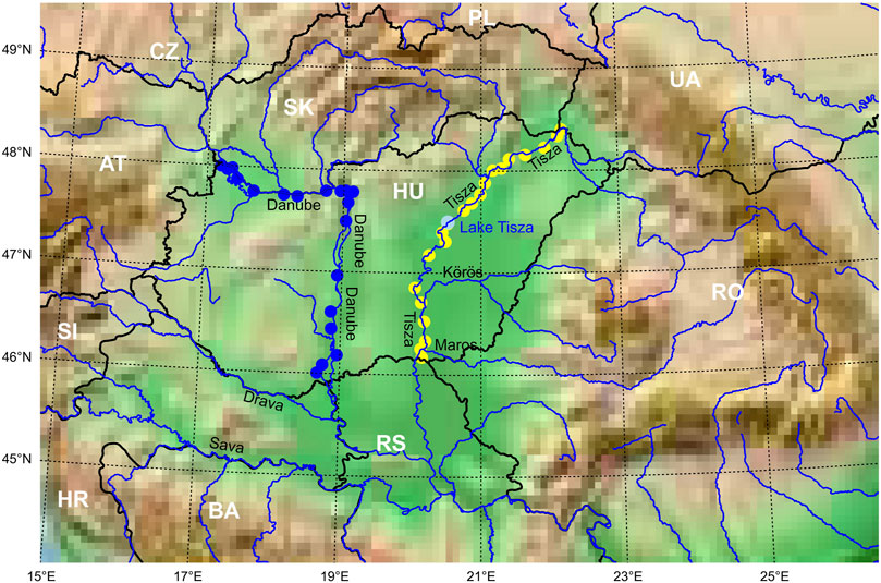
Figure 1. Hydrometric stations along the Danube (blue symbols) and Tisza (yellow symbols). The map illustrates the whole Carpathian Basin, political borders are black, country codes are white, and major rivers are blue lines. Two large tributaries of the Tisza are labeled (Körös and Maros), the same is for the Danube (Drava and Sava). The map was constructed by the Python (ver. 3.8.8) module Basemap (1.3.2) https://matplotlib.org/basemap.

The Carpathian Basin makes up a significant part of the Danube drainage basin, where the river changes its character to a lowland section, while the entire drainage basin of the Tisza river is located in the basin (Sommerwerk et al., 2022; Gâştescu, 1998). Except for the study by Jánosi et al. (2023), which serves as a precursor to this article, no such comprehensive statistical analysis has been carried out for water stations in Hungary. The statistical analyses of Konecsny and Nagy (2014) for the Danube and the Tisza were limited to a single station, the former in Nagymaros and the latter in Szeged. In the present study, Nagymaros is also among the 19 Danube stations analysed, while among the 22 stations on the Tisza, the station in Csongrád is very close to the station in Szeged.

The catchment basins in Hungary contribute to the hydrological system of the two principal rivers, the Danube and its tributary, the Tisza, except for a few smaller streams (Szlávik, 2005; Nike et al., 2010; Borics et al., 2016). These two major streams, with a combined length of 2,822 km, effectively drain the entire territory of Hungary, which spans 93,000 ${\text{km}}^2$. The rivers that reach the Hungarian border carry water from an area of 290,000 ${\text{km}}^2$, three times larger than Hungary itself. Consequently, the flow patterns in these rivers are primarily influenced by the hydrometeorological events occurring in their upstream regions (Szlávik, 2005; Nike et al., 2010; Hein et al., 2019; Szolgay et al., 2020; Jánosi et al., 2023). Lowland river sections share the property of minor natural falls resulting in slowing river flow speeds and complicated sediment transport. Dams have a far-reaching back swelling effect in the upstream direction.

Figure 2 shows two long time series (121 years of daily water levels) recorded at two stations from the upper section of the Tisza River. Albeit it seems appealing to analyze such long records (where it is available), the plots illustrate significant problems with the data series. Lack of observations for a couple of years is common, not to mention the apparent jumps in low-water levels in both series. Particularly in Figure 2B, the jump in the late fifties coincides with the start of operation (1958) at the Tiszalök Dam (518.225 river km), where the back swelling effect reaches over 80 km upstream (Bezdán, 2010). Tiszabercel (569.0 river km) is some 50 river km up from Tiszalök, where low water levels increased by about 270 cm (Figure 2B). Note that homogenization cannot help in similar situations, the upper envelope (high water levels) did not really change. For these reasons, the research restricts the further analysis to the last two-three decades (red coloring in Figure 2), when high-frequency measurements are also available. In the main text, only representative examples are shown, the whole set of 22 stations for Tisza and 19 stations for Danube (water levels and river discharges) are presented in (Supplementary Material from now on).

Figure 2

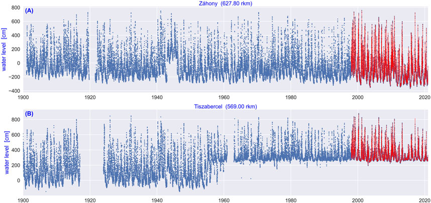
Figure 2. Two long time series (121 years) of water levels at the upper Tisza. (A) Záhony (627.8 river km), and (B) Tiszabercel (569 river km). Besides the lack of data common in both records, low-water data in (B) exhibit a marked increase since the end of the fifties when the Tiszalök Dam (518.225 river km) started operation. Since the natural fall of the river section between Záhony and Tokaj is the smallest (only a couple of cm/km), the back swelling limit is as far as 80 km upstream from the Tiszalök Dam. The red sections in the past 25 years indicate the target of our statistical analysis based on high-resolution.

Some further problems with the data are illustrated in Figure 3. The paper intentionally shows Figure 3B (Tiszafüred, 430.5 river km), which represents a highly regulated section of the Tisza. This hydrometric station is about 26.5 rkm up from the Kisköre Dam (or Tisza Dam); therefore, the water level is around 550 cm during the largest part of each year, apart from extreme low-water and flood situations. The research did not ignore such records from its analysis (for an even stronger regulated example, see Supplementary Figure S1K, Kisköre-Felső), because the whole river is rather distinct from a free-flow stream with its 1800 structures (sluices, culverts), which cross the levees (Szlávik, 2005).

Figure 3

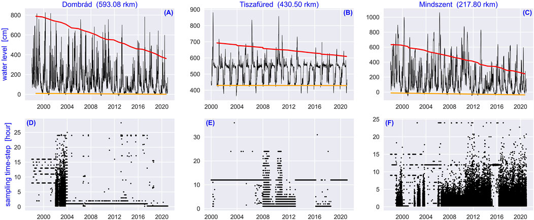
Figure 3. Water level time series and sampling time-step records for three representative stations along the Tisza River. (A, D): Dombrád (upper Tisza); (B, E): Tiszafüred (an example of a strongly regulated section); (C, F): Mindszent (lower Tisza). The same results are shown for the full set of 22 stations in Supplementary Figures S1, S2. Annual maxima and minima of water levels are fitted by a Theil-Sen estimator. Slopes are the following. (A): −9.937 cm/year (red), −0.38 cm/year (orange); (B): −4.14 cm/year (red), −0.04 cm/year (orange); (C): −18.07 cm/year (red), −1.13 cm/year (orange).

Figures 3D–F illustrate another problematic aspect of hydrological time series: the hectic sampling. Sampling time steps change between 15 min and 30 h randomly. Longer breaks are infrequent; therefore, essential events such as floods are not probable to be missed (see also Supplementary Figures S2, S4, S6). Some well-known standard statistical methods require even sampling. To overcome uneven sampling, we implemented a resampling procedure using interpolation and down-sampling (in periods of too frequent sampling) to produce homogeneous series. Cubic spline interpolation and resampling were performed by routines in the SciPy library in Python (Virtanen et al., 2020, Python Programming Language (RRID: SCR_008394)]. For the third-degree spline, the error due to the Runge phenomenon is still relatively small. The results are illustrated in Figure 4. Here a short part of an unevenly sampled record (Tuzsér, 613.9 river km, see Supplementary Figure S1U) is shown (black stars at the top) with resampled homogeneous series are various time steps between 15 min and 1 day. Fine details are also well represented even in the highest frequency case of 15 min.

Figure 4

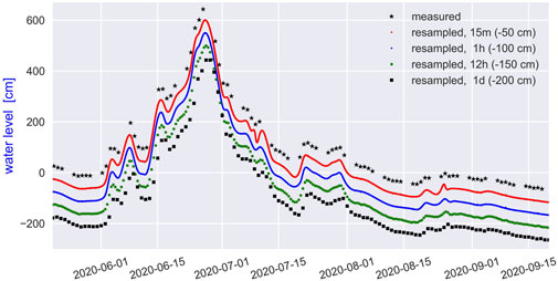
Figure 4. 123 days long time series (black stars) and its resampled versions for various time steps by cubic spline interpolation. Red: 15 min, blue: 1 h, green: 12 h, and black squares: 1 d. The resampled series are shifted down by 50–50 cm for better visualization; see legend. The station is Tuzsér (613.9 river km, upper Tisza), Supplementary Figure S1U. Note the irregular sampling with gaps of a couple of full days (black stars at the top).

2.2 Data processing and methods

Most of the calculations in our statistical analyses were performed in a Python environment (version 3.6, RRID: SCR_008394) with the standard Numpy (Harris et al., 2020) and Scipy (Virtanen et al., 2020, RRID: SCR_008058) packages. The map of Figure 1 is drawn by the Basemap module (https://matplotlib.org/basemap/, last accessed on 02/08/2023). There are a few procedures specifically created to handle unevenly sampled time series. For example, the paper performed frequency analyses using the Lomb–Scargle periodogram method (Press and Rybicki, 1989; VanderPlas, 2018). A naive use of Fourier transform indeed fails for such data. The algorithm provides harmonic fits to the input time series in the form

$s\left(t_i\right)={\displaystyle \sum _{i=1}^k}{a}_i\sin \left({\omega }_{i}t-\phi \right)+b_i\cos \left({\omega }_{i}t-\phi \right)+c_i(1)$

where $s(t_i)$ represents the fitted coordinates of each time $t_i$; $c_i$ is the noise term, $a_i$ and $b_i$ denote the amplitudes of sine and cosine functions of the $i$th harmonic, $\phi$ is the phase factor needed to orthogonalize sin and cosine, and ${\omega }_i$ represents the corresponding angular frequency (the mean value of the signal is removed prior the fitting). The quality of the fit according to Equation 1 defines the Lomb-Scargle amplitudes. The Python routine LombScargle() from the package Astropy was installed (Astropy Collaboration et al., 2022). Note that the statistical significance of peaks is difficult to determine, we used the time-consuming procedure of determining “false alarm probabilities” by the “bootstrap” method VanderPlas (2018). The “false alarm probability” concept answers a particular question (VanderPlas, 2018): What is the probability that a time series with no periodic component (white noise) would lead to a peak of a given magnitude? Since the records can be considered long oversampled series with smooth and correlated increments and decrements, the false alarm probabilities are so small (in the order of ${10}^{-3}$ or less) that they cannot be distinguished from zero (If the probability level of a false result is set at $P$, then the number of runs $n_b\approx 10/P$.)

Traditional Fourier and Welch periodograms were also estimated after resampling the records with a time step of 1 h, as described above (see Figure 4. In the Welch method, a sliding window (width is an input parameter) moves along the signal (usually with half overlaps), and the windowed spectrum is averaged from these different samples. When the width of the window is too small, lower frequency peaks are not resolved. In the opposite case, too wide windows result in a result close to a discrete Fourier transform. The use of the Welch method is justified in case the window of choice $(D)$ is set at $D=M/2$ relative to the natural time interval $(M)$ If the width of the window is decreased, it leads to a limit transition to Bartlett’s method, if it is increased, to Fourier analysis. Confidence intervals cannot be estimated easily again because water level and discharge time series are not uncorrelated stochastic processes.

Linear fits do not require even sampling. The Theil-Sen robust linear estimator routine [Python, SciPy package, scipy.stats.mstats.theilslopes() routine (Virtanen et al., 2020)] was implemented because this algorithm is known to ignore outliers very effectively (Akritas et al., 1995; Eugster et al., 2022). The fitted line has the median of the slopes of all lines through all pairs of points. The Theil-Sen algorithm has a breakdown point of about 29.3% (the ratio of arbitrary outliers) in the case of simple linear regression.

Water level and river discharge changes are estimated from resampled time series with a step of 12 h. It is meaningless to evaluate the original records because of the hectic sampling. The semilogarithmic histograms of 12 h changes can be well fitted by a piecewise linear function, which means a piecewise exponential behavior for the original data:

$\ln \left[y\left(x\right)\right]=\left\{\begin{array}{cc}{k}_{1}x+y_0-k_1{x}_0\hfill & \text{if}x<x_0\hfill \\ k_{2}x+y_0-k_2{x}_0\hfill & \text{if}x\ge x_0\hfill \end{array}\right.(2)$

where $k_1$ and $k_2$ are slopes, and $(x_0,y_0)$ is the location of the breaking point. Since piecewise fits are nonlinear, required input parameters are approximate guess values (actually, the success depends strongly on the initial guess). Calculations were performed by the curve_fit algorithm from the SciPy.optimize module (Virtanen et al., 2020). Absolute values of the negative steps were separately evaluated.

3 Results

In this Section, the results of statistical analysis will be presented for the 22 stations along the Tisza (water levels) and the 19 stations along the Danube (water levels and river discharges). Most of the data extends longer than the past two decades. During this period, Europe suffered from faster warming than the global average (Klein Tank et al., 2002; Menne et al., 2012; Lorenz et al., 2019; Naumann et al., 2021; Rousi et al., 2022; Szöllősi-Nagy, 2022), which affects water temperatures as well (Zweimüller et al., 2008; Bui et al., 2018). The Carpathian Basin is not an exception clearly indicated by evaluations of hourly or daily temperatures (Lakatos et al., 2021a; Lakatos et al., 2021b; Barna et al., 2022), extreme values (Lakatos et al., 2014; Bartholy and Pongrácz, 2007) or the frequency of warm spells (Lakatos et al., 2014; Bokros and Lakatos, 2022). An immediate consequence of global climate change is that time series lose stationarity, as it was shown in several cases. Note that nonstationarities cannot be simply handled by removing some linear or nonlinear trends or seasonalities in several cases, e.g., water levels in the Tisza River exhibit a decreasing tendency of high-water levels, while low-water levels do not change (see below).

3.1 Time series and long-time mean values

In Figure 3, water level time series and sampling time-step records have already been plotted for three representative stations along the Tisza River; all the 22 stations are illustrated in Supplementary Figures S1–S2. Annual maxima (red lines) and minima of water levels (orange lines) are fitted by a Theil-Sen estimator. The mean slope for the maxima is −9.94 $\pm$3.75 cm/year, for the minima −0.91 $\pm$1.00 cm/year. It is emphasized here that the standard deviations represent the station-to-station variability. Trends in annual extremes are determined by complex processes such as climate change, precipitation regime shifts, river management operations, river bed erosion, infiltration properties, etc. Therefore, a homogeneous behavior is not expected.

As for the Danube, Figures 5, 6 illustrate water level time series and river discharge records for three selected stations, the remaining 16 are shown in Supplementary Figures S3–S6. Annual maxima exhibit less pronounced decreasing tendencies (red lines) than at the Tisza; the mean value and standard deviation are −3.20 $\pm$3.31 cm/year, where only three stations have slight positive tendencies (see Supplementary Figures S3A, D, E), probably because the number of “outliers” is too large. The annual minima obey weak negative mean tendency −1.07 $\pm$1.52 cm/year, nevertheless below Vác (1,679.5 river km) down to Mohács (1,446.9 river km) in Supplementary Figure S3J–Q decrease is the dominating trend. This river section is a part of the second largest free-flowing section of the Danube, where 78 barriers along the whole river are installed. Less than 15% of the Upper Danube remains free-flowing (Nike et al., 2010). Again, trend standard deviations indicate station-to-station variations.

Figure 5

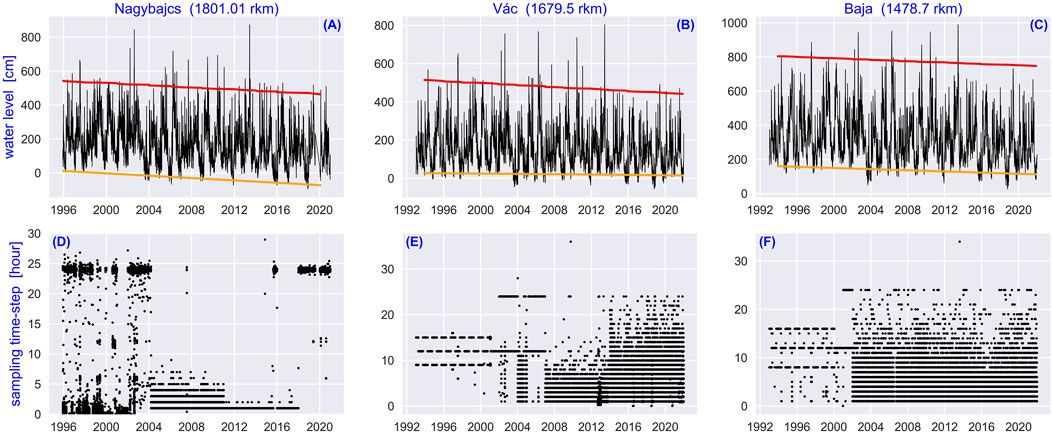
Figure 5. Water level time series and sampling time-step records for three representative stations along the Danube River. (A, D): Nagybajcs (upper Danube); (B, E): Vác (upper Danube, 123 river km away from Nagybajcs); (C, F): Baja (lower Danube). The same results are shown for the full set of 19 stations in Supplementary Figures S3, S4. Annual maxima and minima of water levels are fitted by a Theil-Sen estimator. Slopes are the following. (A): −3.25 cm/year (red), −3.47 cm/year (orange); (B): −2.59 cm/year (red), −0.43 cm/year (orange); (C): −2.06 cm/year (red), −1.70 cm/year (orange).

Figure 6

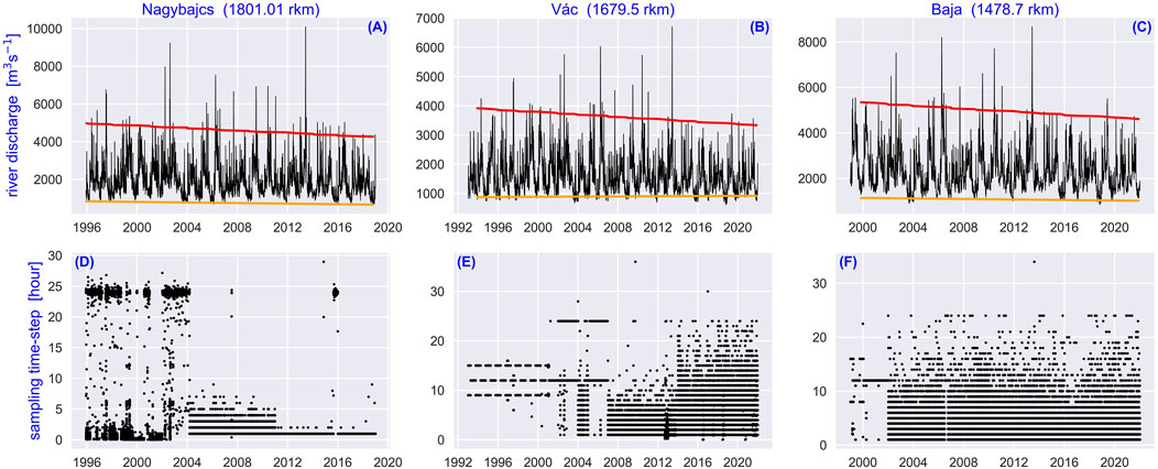
Figure 6. River discharge time series and sampling time-step records for the same three representative stations as in Figure 5 along the Danube River. (A, D): Nagybajcs (upper Danube); (B, E): Vác (upper Danube, 123 river km away from Nagybajcs); (C, F): Baja (lower Danube). The same results are shown for the full set of 19 stations in Supplementary Figures S5, S6. Annual maxima and minima of water levels are fitted by a Theil-Sen estimator. Slopes are the following. (A): −32.05 m³s⁻¹/year (red), −7.78 m³s⁻¹/year (orange); (B): −20.67 m³s⁻¹year⁻¹ (red), 1.64 m³s⁻¹year⁻¹ (orange); (C): −33.18 m³s⁻¹/year (red), −5.65 m³s⁻¹/year (orange).

The same procedures were applied for river discharge data along the Danube, where it was possible; see Figure 6 and Supplementary Figures S5–S6. The behavior along the Danube is very similar to water levels; however, this is strongly expected. Water levels and river discharges are in a functional relationship expressed by the rating curve for a given station and primarily determined by the streambed material and the shape of the river cross-section at the hydrometric station (Zsuffa, 1999; Rhoads, 2020b). This measured nonlinear function is used to estimate discharges from water level data because it is way simpler to read a level gauge than measure discharge in the whole cross-section. Annual maxima and minima are fitted as before; the ensemble mean slopes for 16 stations (see Supplementary Figure S5) are −26.36 $\pm$38.14 ${\text{m}}^3{\text{s}}^{-1}$/year (red lines) and −1.38 $\pm$ 4.81 ${\text{m}}^3{\text{s}}^{-1}$/year (orange lines). Two stations have an increasing tendency for annual maximum discharge, while the annual maximum water levels are decreasing: Dunakiliti (1842.0 river km) and Dunaalmás (1758.1 river km), see Supplementary Figures S5B, G. The first location is a strongly regulated section close to a dam and bottom sill, while the second place is at a more or less free-flowing section. Here the annual minimum discharges also have an anomalous increasing trend with a slope of 9.66 ${\text{m}}^3{\text{s}}^{-1}$/year; an explanation requires further research. The slopes of water level and flow are summarised in Table 1.

Table 1

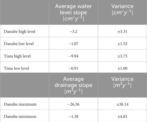
Table 1. Slope of the annual maximum and minimum water level of the Danube and the Tisza, and summary of the slope of the water yield. Changes in water yield data for the Tisza are still missing.Standard deviations represent the station-to-station variability.

Supplementary Figures S7–S9 exhibit the normalized histograms for sampling time frequencies in semilogarithmic plots. Similarly to the temporal distributions, no real patterns are visible. Some histograms have a near-exponential decay for larger gaps, but others are pretty irregular. Note however, that in almost all cases small sampling intervals are absolutely dominating in almost all stations.

Climatic mean values with standard deviations are shown in Figure 7 for 3-3 representative stations for each day of the year; the whole sets of hydrometric stations are evaluated in Supplementary Figures S10–S12. Highly regulated sections can be recognized easily with wide plateaus and damped fluctuations (narrow standard deviation bands). Long-time mean water levels Supplementary Figures S10, S11 have a relatively weak seasonality with significant fluctuations. Higher levels are characteristic in late spring and summer, suggesting that the hydrometeorological circumstances in the upstream sections (outside Hungary) are the determining factors, indeed. Note the substantial similarity between the water level and river discharge mean values for a given station along the Danube; even the fine structure of the fluctuations is very similar. This is expected; the two variables are in a functional relationship, as explained above.

Figure 7

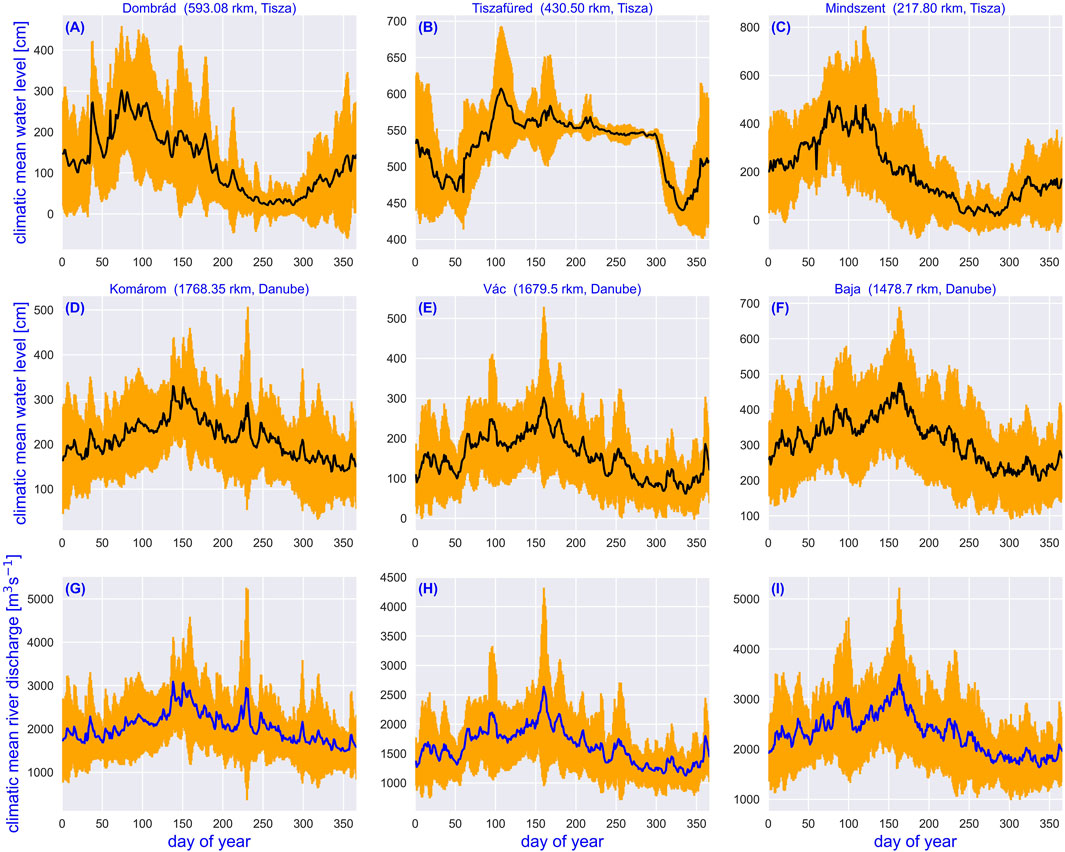
Figure 7. Long-time (climatic) mean with error bar (orange) for 3-3 representative hydrographic stations along the Tisza and the Danube. (A): Dombrád water levels (upper Tisza); (B): Tiszafüred water levels (an example of a strongly regulated section); (C): Mindszent water levels (lower Tisza). The same climatic means are shown for the full set of 22 stations in Supplementary Figure S10. (D) Komárom water levels (upper Danube); (E): Vác water levels (upper Danube, 88 river km away from Komárom); (F): Baja water levels (lower Danube); (G) Komárom river discharges; (H): Vác river discharges; (I): Baja river discharges. The same climatic means are shown for the full set of 19 stations in Supplementary Figures S11, S12.

3.2 Extracting periods

As described in Section 2, relevant periodicities were examined by the Lomb-Scargle algorithm (Press and Rybicki, 1989; VanderPlas, 2018), and results are shown for 3-3 representative stations in Figure 8. The same is presented for all stations in Supplementary Figures S13, S16, S17. The leading period for all records is obviously 1 year. However, some secondary peaks are visible in the spectra. Notably but not unexpectedly, the spectra for Danube stations, both for water levels and river discharges are practically the same, even in fine details (apart from the units, of course). The problem of estimating the statistical significance of candidate periodicities for a number of periodograms is far from trivial.

Figure 8

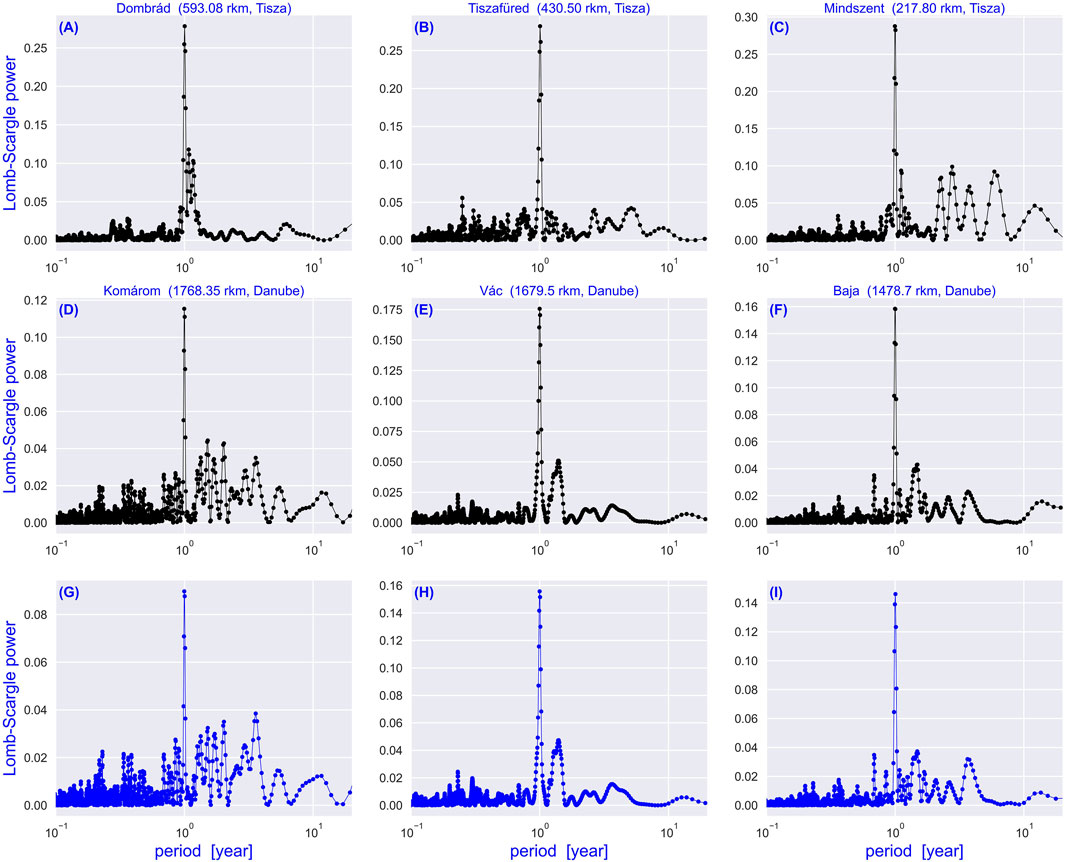
Figure 8. Lomb-Scargle periodograms for 3-3 representative hydrographic stations along the Tisza and the Danube. The horizontal axes are logarithmic. (A): Dombrád water levels (upper Tisza); (B): Tiszafüred water levels (an example of a strongly regulated section); (C): Mindszent water levels (lower Tisza). The same periodograms are shown for the full set of 22 stations in Supplementary Figure S13. (D) Komárom water levels (upper Danube); (E): Vác water levels (upper Danube, 88 river km away from Komárom); (F): Baja water levels (lower Danube); (G) Komárom river discharges; (H): Vác river discharges; (I): Baja river discharges. The same periodograms are shown for the full set of 19 stations in Supplementary Figures S16, S17.

We also implemented two Fourier based methods, the first is the classical power spectrum estimate, the second is the Welch periodogram. The later is essentially Fourier transforms in sliding windows, where the estimate is based on averaging the partial spectra. Figure 9 exhibits illustrative Fourier power spectra for 3-3 stations. Discharge spectra are not shown neither here nor in SuppMat, because they are identical with Danube water levels. Full sets for Fourier and Welch spectra are shown in Supplementary Figures S14, S15 for the Tisza river, and in Supplementary Figures S18, S19 for Danube water levels. All time series are resampled by 1 h steps before employing the Fourier transforms. It is probably essential that resampling did not change the total length of time series because of the domination of high frequency measurements (15 min) with intermittent longer breaks (up to 25–27 h, typically). The Fourier spectra indicate weaker peaks in 15 out of the 22 cases with periods of around 2.3 and 4.6 years for the Tisza, and in 15 out of 19 cases with periods of 1.3–1.5 years for the Danube. Secondary peaks were identified when their amplitude was at least 1/6 of the main peak or larger.

Figure 9

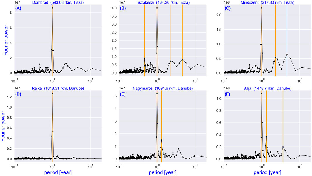
Figure 9. Unnormalized Fourier power spectra for 3-3 representative hydrographic stations along the Tisza and the Danube. The horizontal axes are logarithmic. Time series are resampled with a time-step of 1 h (cubic spline fit and downsampling) prior to feeding them to the FFT algorithm. Vertical orange lines identify periods where the Fourier power is at least one sixth of the maximum value. (A): Dombrád (upper Tisza); (B): Tiszafüred (an example of a strongly regulated section); (C): Mindszent (lower Tisza). The same power spectra are shown for the full set of 22 stations in Supplementary Figure S14. (D) Rajka (upper Danube); (E): Nagymaros (upper Danube, 152 river km down from Rajka 152 river km down from Rajka); (F): Baja water levels (lower Danube). The same periodograms are shown for the full set of 19 stations in Supplementary Figures S16, S17.

Whether the observations reflect natural variabilities or there are some algorithmic artefacts, requires further investigations. The large widths suggest that such periods are not strict oscillatory modes but they rather represent quasi-periodicities. Quasi-periodic oscillations are common in the climate system (see, e.g., Kundzewicz et al., 2019; Börgel et al., 2020; Norel et al., 2021). If it is established that these secondary peaks originate from any cyclical changes in either land use or climate change that are not annual in nature, we may get a better understanding of the impact of these processes on the hydrological cycle. Recently, Briciu and Mihăilă (2014) identified similar periods in a nearby region (Eastern Carpathian) by a wavelet technique, 36 hydrographic signals from the total of 45 exhibited quasi-periodic oscillations between 2.9 and 3.5 years. The authors selected climate oscillation modes with similar characteristic periods: Arctic Oscillation (AOI), East Atlantic Oscillation Index (EAOI), East Atlantic/West Russia Oscillation (EAWROI), NINO3.4, North Atlantic Oscillation Index (NAOI), Southern Oscillation Index (SOI), and West Pacific Oscillation Index (WPOI). However, solid explanations with the mechanisms of teleconnections is a difficult task, again (Briciu and Mihăilă, 2014). Szolgayova et al. (2014) also showed that there are periods other than annual in the upper Danube (Austria and Slovakia), using a similar method to the one presented here (wavelet analysis of frequencies), although the time resolution is much higher: monthly, whereas in our data it is 12 h. Mares et al. (2020) carried out a wavelet analysis for the Romanian section of the Danube, also similar to our work, looking for periods other than the annual periodicity. Their data series had a monthly resolution and a length of 52 years. See Table 2.

Table 2

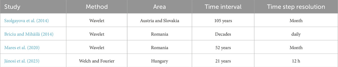
Table 2. Water yield and water level periodicity studies on the Danube.

3.3 Statistics of 12 h changes in water levels and river discharges

Time derivatives of a data series have the appealing property that they are close to be stationer (variability still might change in time, known as volatility clustering in financial literature). Water level and discharge change statistics cannot be reliable at hectic sampling time intervals, therefore empirical histograms were determined after resampling the original records with a time step of 12 h. Representative examples are illustrated in Figure 10, note the semi-logarithmic scales. Full sets are shown in Supplementary Figures S21–S23. A visual inspection of the curves suggested that piecewise-exponential fits should work, therefore we used Equation 2. For the tests. Note that any piecewise fit is nonlinear, therefore it does not work without providing appropriate initial guess values for the parameters. Since Equation 2 describes fits with a common breakpoint for the parts (one for the positive and one for the negative sides of histograms), these (approximate) locations are also input parameters. Before the fitting, the negative sides of the histograms were properly transformed.

Figure 10

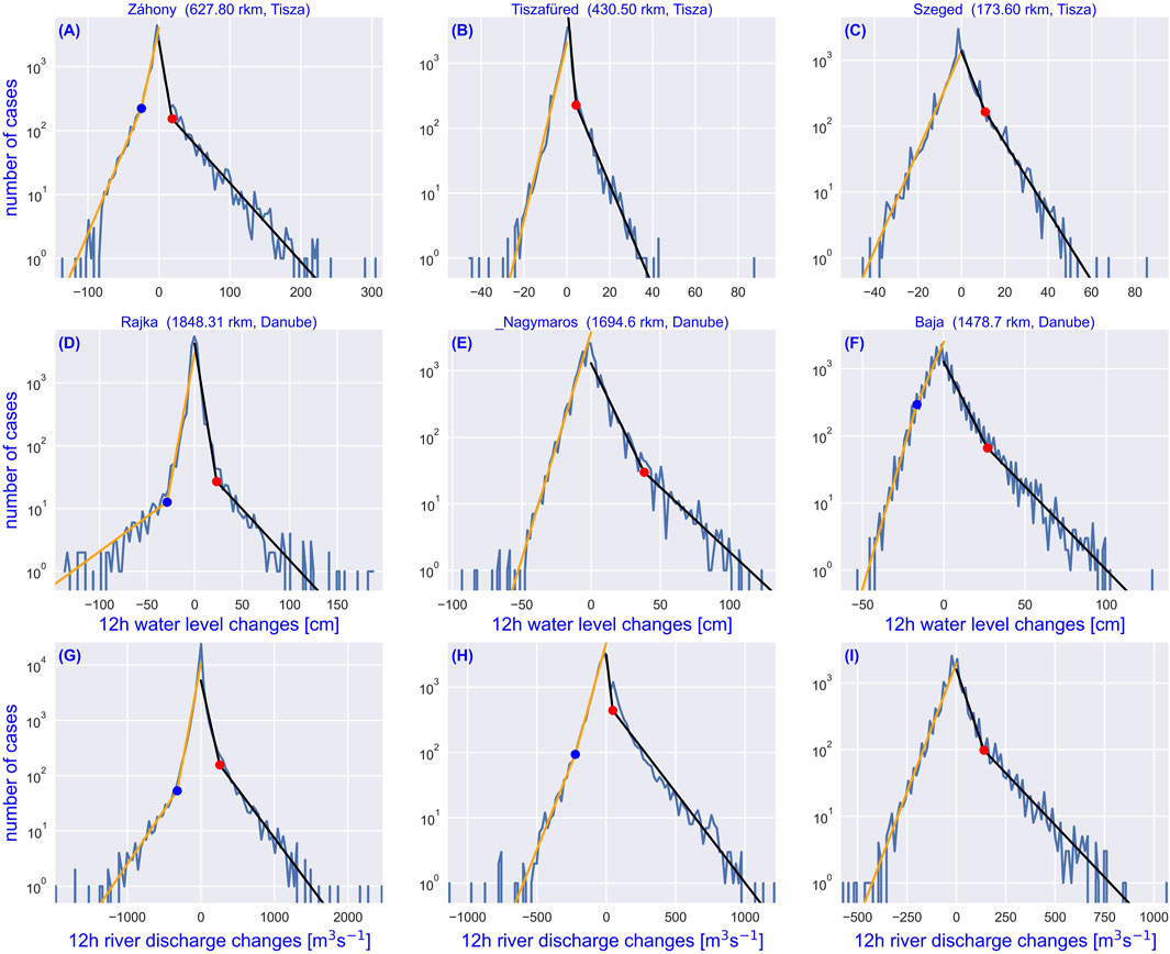
Figure 10. Histograms of 12 h changes and piecewise-exponential fits for 3-3 representative hydrographic stations along the Tisza and the Danube. Time series are resampled with a time-step of 12 h (cubic spline fit and downsampling) before backward differences are determined. Black/orange lines denote the piecewiseexponential fits for the positive/negative sides of the histograms, breaking points are indicated by red/blue symbols (wherever they are detected). (A): Záhony water level changes (upper Tisza); (B): Tiszafüred water level changes; (C): Szeged water level changes (lower Tisza). The same histograms with fits are shown for the full set of 22 stations in Supplementary Figure S18. (D) Rajka water level changes (upper Danube); (E): Nagymaros water level changes (upper Danube, 152 river km down from Rajka); (F): Baja water level changes (lower Danube); (G) Rajka river discharge changes; (H): Nagymaros river discharge changes; (I): Baja river discharges. The same histograms are shown for the full set of 19 stations in Supplementary Figures S19, S20.

The result indicate that behavior is quiet universal for each station. Usually a broken exponential fit works nicely for both sides, however in many cases, the negative step sizes (water level and river discharge drops) exhibit a simple exponential decay. This behavior is expected. We mentioned that hydrographs do not represent a stochastic process, actually they are changing smoothly as described in all related textbook (Rhoads, 2020a; Rhoads, 2020b). Rising and falling limbs (after a precipitation event or flood wave) are steep with larger steps, close to the saturation steps are much smaller.

As for the fitted parameters, slopes and breaking points are scattered in a wide range. This is the consequence of large deviations in gauge zero levels, the shape of river cross sections, erosional circumstances, etc., station to station. The parameters have importance at local runoff modeling and prediction, which should be tuned to local circumstances. Nevertheless such parameters can be used for calibrations and validations at building models.

3.4 Timing of annual extremes

This point is related to a better understanding the dynamics of various river basins and the effects of regional climate change. Blöschl et al. (2017), Blöschl et al. (2019) extracted regional trends of river “flood” timing and magnitudes in Europe (almost 4,000 records) for five decades from 1960. The data are available at https://github.com/tuwhydro/ (last accessed on 8th of August, 2023). The term “flood” is consistently used in the paper as a proxy for the annual maxima of discharges in each calendar year. The main result is openly available at https://www.eea.europa.eu/data-and-maps/figures/observed-regional-trends-of-annual (last accessed on 8th of August, 2023). Different regions are affected by different primary drivers. 1) Northwestern Europe: Increasing rainfall and soil moisture. 2) Southern Europe: decreasing precipitation and increasing evaporation. 3) Eastern–Northeastern Europe: decreasing precipitation and earlier snowmelt. The area of the Carpathian Basin belongs to subregion 2 with a decreasing annual maximum discharge rate tendency of 5%–12% per decade. value.

Our data exhibit a somewhat controversial behavior. Figure 11 illustrates the day of the year where annual maxima are recorder bot for the Tisza and Danube, the full data sets are presented in Supplementary Figures S21, S23. In order to check consistencies and to avoid the effects of random errors, we determined both single day and the middle date of non-overlapping 5-day maxima. The coincidence is almost perfect, also with the Theil-Sen trends fitted separately. Maxima for the Tisza has an increasing, while for the Danube a decreasing tendency (with a few exceptions). Nevertheless, the scatter around the trends is very large. We evaluated the annual minima as well, examples are in Figure 12. Particularly interesting is the comparison between the two rivers: While annual minima happen regularly at the end of the year along the Tisza, the Danube exhibits two disconnected sets, one at the beginning and one for the end of the year. Minima have no significant trends in timing. Further studies are needed to understand what leads to different trends in the intra-annual location of the day of maximum discharge for the two rivers, although again it should be noted that statistically these fits have a large scatter.

Figure 11

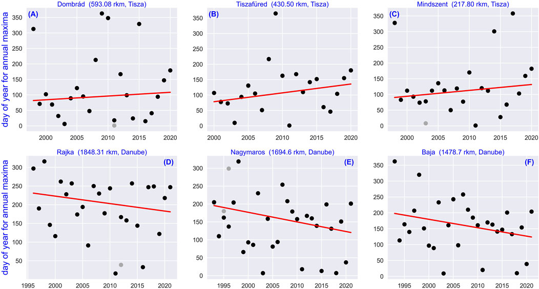
Figure 11. Day of the year for annual maximum water levels for 3-3 representative hydrographic stations along the Tisza and the Danube. Red lines indicate Theil-Sen linear fits. (A): Dombrád (upper Tisza); (B): Tiszafüred (an example of a strongly regulated section); (C): Mindszent (lower Tisza). The same statistics are shown for the full set of 22 stations in Supplementary Figure S21. The mean slope for all stations is 2.32 ± 1.49 days/year (which means almost 50 days of shift during two decades). (D) Rajka (upper Danube); (E): Nagymaros (upper Danube, 152 river km down from Rajka); (F): Baja (lower Danube). The same statistics are shown for the full set of 19 stations in Supplementary Figure S23. The mean slope for all stations is −2.48 ± 1.07 days/year (which means almost −50 days of shift during two decades).

Figure 12

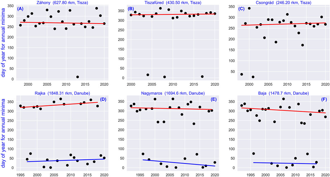
Figure 12. Day of the year for annual minimum water levels for 3-3 representative hydrographic stations along the Tisza and the Danube. Red and blue lines indicate Theil-Sen linear fits. (A): Záhony (upper Tisza); (B): Tiszafüred (an example of a strongly regulated section); (C): Csongrád (lower Tisza). The same statistics are shown for the full set of 22 stations in Supplementary Figure S22. The mean slope for all stations is 0.29 ± 1.10 days/year (D) Rajka (upper Danube); (E): Nagymaros (upper Danube, 152 river km down from Rajka); (F): Baja (lower Danube). The same statistics are shown for the full set of 19 stations in Supplementary Figure S24. Theil-Sen linear fits are plotted separately for the apparent winter-spring (red lines) and late-autumn sets (blue lines). The mean slopes for all stations are −0.45 ± 0.98 (red) and −0.72 ± 1.34 days/year (blue).

4 Results

The detailed statistical analyses was presented for 22 water level records along the Tisza River, and for $19\times 2$ time series for the Danube (where both water level and river discharge measurements were available). We intentionally incorporated stations of strong water management (e.g., close to dams); however, none of the two lowland river sections in Hungary can be really considered as free flow streams. Extensive use for agricultural, industrial and domestic purposes impact strongly any hydrological parameters. Furthermore, lowland rivers have very small natural falls which has a consequence that most of the constructions have far reaching impacts both upward and downward. The Danube has a much larger basin, local hydrometeorological circumstances have dampened effects. The basin of the Tisza is considered as part of the Danube watershed, however the confluence is in Serbia, therefore the Hungarian sections are separated for the two rivers. Particular difficulty is that sampling has a very hectic timing, but this is more or less common everywhere in the world.

The main findings are the following (see also Jánosi et al., 2023):

$•$ Maximum water levels and discharges have a decreasing trend during the past decades. This is most probably the consequence of an accelerated climate change during the same period. Warming decreases winter snow in the mountains, triggers earlier melting, and increases water holding capacity in the atmosphere (increases evaporation rates).

$•$ Minimum water levels and discharges obey less significant trends. This might be related to the fact that almost all rivers arrive from abroad, and both the Tisza and Danube, and most of their tributaries origin from mountainous regions.

$•$ Long time climatological means have a rather weak annual periodicity with very large standard deviations in each calendar day. Maximum water levels and discharges have somewhat higher probability during the first half of a given year.

$•$ We implemented the Lomb-Scargle algorithm to extract characteristic oscillations. Besides an annual periodicity, this procedure cannot clearly resolve smaller amplitude and wide sub-peaks.

$•$ In order to overcome the problems of strongly uneven sampling, we introduced a resampling procedure. This contains two steps: downsampling where the time steps are short, and cubic interpolation for longer gaps than the required interval.

$•$ Resampling permitted to test the standard Fourier and Welch decompositions. The spectra revealed quasi-periodic sub-components of the signals with peaks 2.3 and 4.6 years for the Tisza, and about 1.3–1.5 years for the Danube. Further research is required to check the statistical significances, and to find an explanation of such smeared oscillations, when they exist.

$•$ Resampling also made possible to evaluate the empirical frequency distributions of step sizes of water level and discharge changes. An almost universal behavioris obtanied with a piecewise exponential distribution. Surprisingly, the shape is the same for records of strongly regulated sections. Nevertheless, the fitted parameters change very strongly site to site.

$•$ Finally, we evaluated possible trends of the timing of annual extrema. Maximum values have positive tendencies for the Tisza, while negative ones for the Danube. Annual minima do not show temporal shifting. The later or earlier peak values indicate some regional climate changes which are different for the two basins.

Some limitations exist in this paper, which will impact its analysis and interpretation for the trend of water level and discharge. These processes irregularly sampled time series data from these hydrometric stations, hence causing complications in analyzing and interpreting trends. Another limitation is that high-frequency data are only available for a limited time period. Although this study gives central focus to periods of the last two to 3 decades, the research summarized in Table 2 covered longer periods; time resolution, however, was also a limiting factor in that study. At last, particular methodological approaches are required for the different challenges that unevenly sampled data.

5 Summary

Empirical studies similar to this research are believed to contribute to the validation and calibration of local runoff models, which are widely used in contemporary hydrology and can aid in flood and inland water protection, agriculture and landscape management. All the sectors in this list are affected by extreme weather events and climate change itself, so the importance of this research is evident. The analysis of both water levels and flow rates is important, as is the appearance of periods in the data series that differ from the annual periodicity. The studies summarised in Table 2 also show that the invesigation of the time series of water yield and water level for the Danube and the Tisza, but especially the research on recurrent phenomena different from the annual period is timely and relevant. It helps to understand the climatic cycles that influence the course of rivers and are affected by climate change. Other large European rivers, such as the Volga, the Rhine, the Vistula and the Don, have also been studied, partly with similar content and purpose (Table 3). These studies point to the importance of these hydrological studies for fisheries, conservation of natural systems and mitigation of climate change.

Table 3

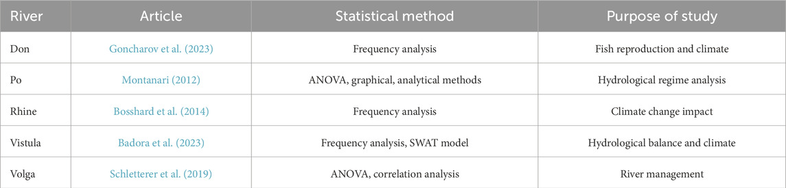
Table 3. Table of hydrological studies of some European rivers.

Data availability statement

Publicly available datasets were analyzed in this study. This data can be found here: https://www.ovf.hu/en/.

Author contributions

IJ: Conceptualization, Formal Analysis, Investigation, Methodology, Software, Validation, Visualization, Writing–original draft. IZ: Conceptualization, Writing–original draft. TB: Conceptualization, Methodology, Writing–original draft. BL: Data curation, Resources, Writing–original draft. AS-N: Conceptualization, Methodology, Writing–original draft. ZH: Formal Analysis, Investigation, Methodology, Resources, Software, Supervision, Validation, Writing–review and editing.

Funding

The author(s) declare that financial support was received for the research, authorship, and/or publication of this article. This research was supported by the Max-Planck-Institute for the Physics of Complex Systems, Germany (Visitor Programme), and by the National Research, Development and Innovation Office, Hungary (grant number K-125171).

Acknowledgments

The help of Mátyás Mérő during the language check and editing is kindly appreciated.

Conflict of interest

Author IZ is employed by Water Resources Research Centre (VITUKI) Hungary Ltd.

The remaining authors declare that the research was conducted in the absence of any commercial or financial relationships that could be construed as a potential conflict of interest.

Publisher’s note

All claims expressed in this article are solely those of the authors and do not necessarily represent those of their affiliated organizations, or those of the publisher, the editors and the reviewers. Any product that may be evaluated in this article, or claim that may be made by its manufacturer, is not guaranteed or endorsed by the publisher.

Supplementary material

The Supplementary Material for this article can be found online at: https://www.frontiersin.org/articles/10.3389/feart.2025.1391458/full#supplementary-material

Footnotes

¹The color of the original text is black, all changes due to the review process are blue

References

Akritas, M. G., Murphy, S. A., and Lavalley, M. P. (1995). The Theil-Sen estimator with doubly censored data and applications to astronomy. J. Amer. Stat. Assoc. 90, 170–177. doi:10.1080/01621459.1995.10476499

CrossRef Full Text | Google Scholar

Astropy Collaboration Price-Whelan, A. M., Lim, P. L., Earl, N., Starkman, N., Bradley, L., et al. (2022). The Astropy Project: sustaining and growing a community-oriented open-source project and the latest major release (v5.0) of the core package. Astrophys. J. 935, 167. doi:10.3847/1538-4357/ac7c74

CrossRef Full Text | Google Scholar

Ayat, H., Evans, J. P., Sherwood, S. C., and Soderholm, J. (2022). Intensification of subhourly heavy rainfall. Science 378, 655–659. doi:10.1126/science.abn8657

PubMed Abstract | CrossRef Full Text | Google Scholar

Badora, D., Wawer, R., Król-Badziak, A., Nieróbca, A., Kozyra, J., and Jurga, B. (2023). Hydrological balance in the vistula catchment under future climates. Water 15, 4168. doi:10.3390/w15234168

CrossRef Full Text | Google Scholar

Bai, Y., Bezak, N., Zeng, B., Li, C., Sapač, K., and Zhang, J. (2021). Daily runoff forecasting using a cascade long short-term memory model that considers different variables. Water.Resour. Manage. 35, 1167–1181. doi:10.1007/s11269-020-02759-2

CrossRef Full Text | Google Scholar

Bárdossy, A., and El Hachem, A. (2021). “Assessment of water quantity,” in Handbook of water resources management: discourses, concepts and examples. Editors J. J. Bogárdi, J. Gupta, K. D. W. Nandalal, L. Salamé, R. R. van Nooijen, N. Kumaret al. (Cham, Switzerland: Springer International Publishing). doi:10.1007/978-3-030-60147-8_14

CrossRef Full Text | Google Scholar

Barna, Z., Izsák, B., and Ildikó, P. (2022). Trend analysis: country-wise temperature trend of hourly values (in Hungarian). Légkör Atmos. 67, 122–129. doi:10.56474/legkor.2022.3.1

CrossRef Full Text | Google Scholar

Bartholy, J., and Pongrácz, R. (2007). Regional analysis of extreme temperature and precipitation indices for the carpathian basin from 1946 to 2001. Glob. Planet. Change 57, 83–95. doi:10.1016/j.gloplacha.2006.11.002

CrossRef Full Text | Google Scholar

Bertola, M., Viglione, A., Lun, D., Hall, J., and Blöschl, G. (2020). Flood trends in europe: are changes in small and big floods different? Hydrol. Earth Syst. Sci. 24, 1805–1822. doi:10.5194/hess-24-1805-2020

CrossRef Full Text | Google Scholar

Beven, K. J. (2011). Rainfall-runoff modelling: the primer. Hoboken, NJ, US: John Wiley and Sons.

CrossRef Full Text | Google Scholar

Bezdán, M. (2010). Characteristics of the flow regime along the regulated Tisza river reach downstream of Tiszafüred. J. Environ. Geogr. 3, 25–30. doi:10.14232/jengeo-2010-43784

CrossRef Full Text | Google Scholar

Blöschl, G., Hall, J., Parajka, J., Perdigão, R. A. P., Merz, B., Arheimer, B., et al. (2017). Changing climate shifts timing of european floods. Science 357, 588–590. doi:10.1126/science.aan2506

PubMed Abstract | CrossRef Full Text | Google Scholar

Blöschl, G., Hall, J., Viglione, A., Perdigão, R. A. P., Parajka, J., Merz, B., et al. (2019). Changing climate both increases and decreases european river floods. Nature 573, 108–111. doi:10.1038/s41586-019-1495-6

PubMed Abstract | CrossRef Full Text | Google Scholar

Bogárdi, J. J., and Fekete, B. M. (2021). “Water: a unique phenomenon and resource,” in Handbook of water resources management: discourses, concepts and examples. Editors J. J. Bogárdi, J. Gupta, K. D. W. Nandalal, L. Salamé, R. R. van Nooijen, N. Kumaret al. (Cham, Switzerland: Springer International Publishing). doi:10.1007/978-3-030-60147-8_2

CrossRef Full Text | Google Scholar

Bokros, K., and Lakatos, M. (2022). Hőségperiódusok vizsgálata Magyarországon a XX. század elejétől napjainkig. Légkör Atmos. 67, 130–140. doi:10.56474/legkor.2022.3.2

CrossRef Full Text | Google Scholar

Booij, M. J. (2005). Impact of climate change on river flooding assessed with different spatial model resolutions. J. Hydrology 303, 176–198. doi:10.1016/j.jhydrol.2004.07.013

CrossRef Full Text | Google Scholar

Börgel, F., Frauen, C., Neumann, T., and Meier, H. E. M. (2020). The atlantic multidecadal oscillation controls the impact of the North Atlantic oscillation on North European climate. Environ. Res. Lett. 15, 104025. doi:10.1088/1748-9326/aba925

CrossRef Full Text | Google Scholar

Borics, G., Ács, É., Boda, P., Boros, E., Erős, T., Grigorszky, I., et al. (2016). Water bodies in Hungary — an overview of their management and present state. Hung. J. Hydrol. 96, 57–67.

Google Scholar

Bosshard, T., Kotlarski, S., Zappa, M., and Schär, C. (2014). Hydrological climate-impact projections for the rhine river: gcm–rcm uncertainty and separate temperature and precipitation effects. J. Hydrometeorol. 15, 697–713. doi:10.1175/JHM-D-12-098.1

CrossRef Full Text | Google Scholar

Briciu, A.-E., and Mihăilă, D. (2014). Wavelet analysis of some rivers in SE Europe and selected climate indices. Environ. Monit. Assess. 186, 6263–6286. doi:10.1007/s10661-014-3853-z

PubMed Abstract | CrossRef Full Text | Google Scholar

Bui, M., Kuzovlev, V., Zhenikov, Y., Füreder, L., Seidel, J., and Schletterer, M. (2018). Water temperatures in the headwaters of the volga river: trend analyses, possible future changes, and implications for a pan-european perspective. River Res. Appl. 34, 495–505. doi:10.1002/rra.3275

CrossRef Full Text | Google Scholar

Chang, F.-J., Chang, L.-C., and Chen, J.-F. (2023). Artificial intelligence techniques in hydrology and water resources management. Water 15, 1846. doi:10.3390/w15101846

CrossRef Full Text | Google Scholar

Cho, M., Kim, C., Jung, K., and Jung, H. (2022). Water level prediction model applying a long short-term memory (LSTM) - gated recurrent unit (GRU) method for flood prediction. Water 14, 2221. doi:10.3390/w14142221

CrossRef Full Text | Google Scholar

Clark, C. (1987). Deforestation and floods. Environ. Conserv. 14, 67–69. doi:10.1017/S0376892900011127

CrossRef Full Text | Google Scholar

Devia, G. K., Ganasri, B., and Dwarakish, G. (2015). A review on hydrological models. Aquat. Procedia 4, 1001–1007. doi:10.1016/j.aqpro.2015.02.126

CrossRef Full Text | Google Scholar

Eugster, W., DelSontro, T., Laundre, J. A., Dobkowski, J., Shaver, G. R., and Kling, G. W. (2022). Effects of long-term climate trends on the methane and CO2 exchange processes of Toolik Lake, Alaska. Front. Environ. Sci. 10. doi:10.3389/fenvs.2022.948529

CrossRef Full Text | Google Scholar

Fekete, B. M., Andreu, A., Argent, R., Avellán, T., Birkett, C., Caucci, S., et al. (2021). “Observations, monitoring and data management,” in Handbook of water resources management: discourses, concepts and examples. Editors J. J. Bogárdi, J. Gupta, K. D. W. Nandalal, L. Salamé, R. R. van Nooijen, N. Kumaret al. (Cham, Switzerland: Springer International Publishing). doi:10.1007/978-3-030-60147-8_13

CrossRef Full Text | Google Scholar

Gâştescu, P. (1998). Danube RiverDanube river: hydrology and geography. Dordrecht: Springer Netherlands, 159–161. doi:10.1007/1-4020-4497-6_53

CrossRef Full Text | Google Scholar

Ghil, M., Allen, M. R., Dettinger, M. D., Ide, K., Kondrashov, D., Mann, M. E., et al. (2002). Advanced spectral methods for climatic time series. Rev. Geophys. 40, 3–1–3–41. doi:10.1029/2000RG000092

CrossRef Full Text | Google Scholar

Goncharov, A. V., Georgiadi, A. G., Milyukova, I. P., Semenova, A. A., Tsyplenkov, A. S., Kireeva, M. B., et al. (2023). Hydrological conditions of phytophilic fish reproduction in the lower don river under the influence of climate change and flow regulation. Hydrobiologia. doi:10.1007/s10750-023-05432-y

CrossRef Full Text | Google Scholar

Guerreiro, S., Fowler, H., Barbero, R., Westra, S., Lenderink, G., Blenkinsop, S., et al. (2018). Detection of continental-scale intensification of hourly rainfall extremes. Nat. Clim. Change 8, 803–807. doi:10.1038/s41558-018-0245-3

CrossRef Full Text | Google Scholar

Harris, C. R., Millman, K. J., van der Walt, S. J., Gommers, R., Virtanen, P., Cournapeau, D., et al. (2020). Array programming with NumPy. Nature 585, 357–362. doi:10.1038/s41586-020-2649-2

PubMed Abstract | CrossRef Full Text | Google Scholar

Hein, T., Funk, A., Pletterbauer, F., Graf, W., Zsuffa, I., Haidvogl, G., et al. (2019). Management challenges related to long-term ecological impacts, complex stressor interactions, and different assessment approaches in the Danube River Basin. River Res. Appl. 35, 500–509. doi:10.1002/rra.3243

CrossRef Full Text | Google Scholar

Hirsch, R. M., Slack, J. R., and Smith, R. A. (1982). Techniques of trend analysis for monthly water quality data. Water Resour. Res. 18, 107–121. doi:10.1029/WR018i001p00107

CrossRef Full Text | Google Scholar

Hrachowitz, M., Savenije, H., Blöschl, G., McDonnell, J., Sivapalan, M., Pomeroy, J., et al. (2013). A decade of predictions in ungauged basins (PUB) — a review. Hydrol. Sci. J. 58, 1198–1255. doi:10.1080/02626667.2013.803183

CrossRef Full Text | Google Scholar

Ibrahim, K. S. M. H., Huang, Y. F., Ahmed, A. N., Koo, C. H., and El-Shafie, A. (2022). A review of the hybrid artificial intelligence and optimization modelling of hydrological streamflow forecasting. Alexandria Eng. J. 61, 279–303. doi:10.1016/j.aej.2021.04.100

CrossRef Full Text | Google Scholar

Jánosi, I. M., Bíró, T., Lakatos, B. O., Gallas, J. A. C., and Szöllősi-Nagy, A. (2023). Changing water cycle under a warming climate: tendencies in the Carpathian Basin. Climate 11, 118. doi:10.3390/cli11060118

CrossRef Full Text | Google Scholar

Jehanzaib, M., Ajmal, M., Achite, M., and Kim, T.-W. (2022). Comprehensive review: advancements in rainfall-runoff modelling for flood mitigation. Climate 10, 147. doi:10.3390/cli10100147

CrossRef Full Text | Google Scholar

Kemter, M., Marwan, N., Villarini, G., and Merz, B. (2023). Controls on flood trends across the United States. Water Resour. Res. 59, e2021WR031673. doi:10.1029/2021WR031673

CrossRef Full Text | Google Scholar

Kemter, M., Merz, B., Marwan, N., Vorogushyn, S., and Blöschl, G. (2020). Joint trends in flood magnitudes and spatial extents across europe. Geophys. Res. Lett. 47, e2020GL087464. doi:10.1029/2020GL087464

PubMed Abstract | CrossRef Full Text | Google Scholar

Kendon, E. J., and Short, C. J. (2023). Variability conceals emerging trend in 100yr projections of UK local hourly rainfall extremes. Nat. Commun. 14, 1133. doi:10.1038/s41467-023-36499-9

PubMed Abstract | CrossRef Full Text | Google Scholar

Kirchner, J. W., Benettin, P., and van Meerveld, I. (2023). Instructive surprises in the hydrological functioning of landscapes. Annu. Rev. Earth Plane. Sci. 51, 277–299. doi:10.1146/annurev-earth-071822-100356

CrossRef Full Text | Google Scholar

Klein Tank, A. M. G., Wijngaard, J. B., Können, G. P., Böhm, R., Demarée, G., Gocheva, A., et al. (2002). Daily dataset of 20th-century surface air temperature and precipitation series for the european climate assessment. Int. J. Climatol. 22, 1441–1453. doi:10.1002/joc.773

CrossRef Full Text | Google Scholar

Konecsny, K., and Nagy, Z. (2014). “Similarities and differences of the hydrological extremes on the duna/danube and tisza/tisa rivers (1921-2012),” in Aerul Si apa: componente ale mediului/air and water: components of the environment (Cluj-Napoca: Cluj-Napoca: Babes-Bolyai University), 134–141.

Google Scholar

Kundzewicz, Z. W., Szwed, M., and Pińskwar, I. (2019). Climate variability and floods—a global review. Water 11, 1399. doi:10.3390/w11071399

CrossRef Full Text | Google Scholar

Laizé, C. L., and Hannah, D. M. (2010). Modification of climate–river flow associations by basin properties. J. Hydrol. 389, 186–204. doi:10.1016/j.jhydrol.2010.05.048

CrossRef Full Text | Google Scholar

Lakatos, M., Bihari, Z., Izsák, B., Annamária, M., and Szentes, O. (2021a). Observed climate change in Hungary (in Hungarian). Légkör Atmos. 66, 10–11. Available at: https://www.Meteorol.hu/downloads.php?fn=/metadmin/newspaper/2022/04/056abbc1a940abd89a3e61da1de4c5cd-legkor-2021-3.pdf.

Google Scholar

Lakatos, M., Bihari, Z., Izsák, B., and Szentes, O. (2021b). Globális és hazai éghajlati trendek, szélsőségek változása: 2020-as helyzetkép. Sci. Secur. 2, 164–171. doi:10.1556/112.2021.00037

CrossRef Full Text | Google Scholar

Lakatos, M., Bihari, Z., and Szentimrey, T. (2014). Signs of climate change in Hungary (in Hungarian). Légkör Atmos. 59, 158–163. Available at: https://www.met.hu/ismeret-tar/kiadvanyok/legkor/index.php?id=436.

Google Scholar

Li, X., Zhang, K., Bao, H., and Zhang, H. (2022). Climatology and changes in hourly precipitation extremes over China during 1970–2018. Sci. Total Env. 839, 156297. doi:10.1016/j.scitotenv.2022.156297

PubMed Abstract | CrossRef Full Text | Google Scholar

Lorenz, R., Stalhandske, Z., and Fischer, E. M. (2019). Detection of a climate change signal in extreme heat, heat stress, and cold in europe from observations. Geophys. Res. Lett. 46, 8363–8374. doi:10.1029/2019GL082062

CrossRef Full Text | Google Scholar

Mares, I., Mares, C., Dobrica, V., and Demetrescu, C. (2020). Comparative study of statistical methods to identify a predictor for discharge at orsova in the lower danube basin. Hydrological Sci. J. 65, 371–386. doi:10.1080/02626667.2019.1699244

CrossRef Full Text | Google Scholar

Menne, M. J., Durre, I., Vose, R. S., Gleason, B. E., and Houston, T. G. (2012). An overview of the global historical climatology network - daily database. J. Atmos. Oce. Technol. 29, 897–910. doi:10.1175/JTECH-D-11-00103.1

CrossRef Full Text | Google Scholar

Montanari, A. (2012). Hydrology of the po river: looking for changing patterns in river discharge. Hydrology Earth Syst. Sci. 16, 3739–3747. doi:10.5194/hess-16-3739-2012

CrossRef Full Text | Google Scholar

Naumann, G., Cammalleri, C., Mentaschi, L., and Feyen, L. (2021). Increased economic drought impacts in europe with anthropogenic warming. Nat. Clim. Change 11, 485–491. doi:10.1038/s41558-021-01044-3

CrossRef Full Text | Google Scholar

Nike, S., Jürg, B., Momir, P., Christian, B., Markus, V., Martin, S.-J., et al. (2010). Managing the world’s most international river: the Danube River Basin. N. Z. J. Mar. Freshw. Res. 61, 736–748. doi:10.1071/MF09229

CrossRef Full Text | Google Scholar

Norel, M., Kałczyński, M., Pińskwar, I., Krawiec, K., and Kundzewicz, Z. W. (2021). Climate variability indices —- a guided tour. Geosci 11, 128. doi:10.3390/geosciences11030128

CrossRef Full Text | Google Scholar

Peng, A., Zhang, X., Xu, W., and Tian, Y. (2022). Effects of training data on the learning performance of LSTM network for runoff simulation. Water Resour. manage. 36, 2381–2394. doi:10.1007/s11269-022-03148-7

CrossRef Full Text | Google Scholar

Ponce, V. M., and Hawkins, R. H. (1996). Runoff curve number: has it reached maturity? J. Hydrol. Eng. 1, 11–19. doi:10.1061/(ASCE)1084-0699(1996)1:1(11)

CrossRef Full Text | Google Scholar

Press, W. H., and Rybicki, G. B. (1989). Fast algorithm for spectral analysis of unevenly sampled data. Astrophys. J. 338, 277–280. doi:10.1086/167197

CrossRef Full Text | Google Scholar

Rhoads, B. L. (2020a). Flow dynamics in rivers. Cambridge University Press, 72–96. doi:10.1017/9781108164108.004

CrossRef Full Text | Google Scholar

Rhoads, B. L. (2020b). Magnitude-frequency concepts and the dynamics of channel-forming events. Cambridge University Press, 134–163. doi:10.1017/9781108164108.006

CrossRef Full Text | Google Scholar

Rousi, E., Kornhuber, K., Beobide-Arsuaga, G., Luo, F., and Coumou, D. (2022). Accelerated western european heatwave trends linked to more-persistent double jets over eurasia. Nat. Commun. 13, 3851. doi:10.1038/s41467-022-31432-y

PubMed Abstract | CrossRef Full Text | Google Scholar

Schletterer, M., Shaporenko, S., Kuzovlev, V., Minin, A., Van Geest, G., Middelkoop, H., et al. (2019). The volga: management issues in the largest river basin in europe. River Res. Appl. 35, 510–519. doi:10.1002/rra.3268

CrossRef Full Text | Google Scholar

Simon, C., Kis, A., and Torma, C. (2023). Temperature characteristics over the carpathian basin-projected changes of climate indices at regional and local scale based on bias-adjusted cordex simulations. Int. J. Climatol. 43, 3552–3569. doi:10.1002/joc.8045

CrossRef Full Text | Google Scholar

Sommerwerk, N., Bloesch, J., Baumgartner, C., Bittl, T., Čerba, D., Csányi, B., et al. (2022). “Chapter 3 - the danube river basin,” in Rivers of Europe. Editors K. Tockner, C. Zarfl, and C. T. Robinson Second Edition (Elsevier), 81–180. doi:10.1016/B978-0-08-102612-0.00003-1

CrossRef Full Text | Google Scholar

Szlávik, L. (2005). “Enhancement of flood safety, rural and regional development in the Hungarian part of the Tisza valley (the new vásárhelyi plan),” in River basin management III. (WIT transactions on ecology and the environment). Editors C. Brebbia, and J. A. D. Carmo (Southampton, UK: WIT Press), 465–474. doi:10.1002/9781119300762.wsts0062

CrossRef Full Text | Google Scholar

Szolgay, J., Blöschl, G., Gribovszki, Z., and Parajka, J. (2020). Hydrology of the Carpathian Basin: interactions of climatic drivers and hydrological processes on local and regional scales – HydroCarpath Research. J. Hydrol. Hydromech. 68, 128–133. doi:10.2478/johh-2020-0017

CrossRef Full Text | Google Scholar

Szolgayova, E., Parajka, J., Blöschl, G., and Bucher, C. (2014). Long term variability of the danube river flow and its relation to precipitation and air temperature. J. Hydrology 519, 871–880. doi:10.1016/j.jhydrol.2014.07.047

CrossRef Full Text | Google Scholar

Szöllősi-Nagy, A. (2022). On climate change, hydrological extremes and water security in a globalized world. Sci. Secur. 2, 504–509. doi:10.1556/112.2021.00081

CrossRef Full Text | Google Scholar

Tarasova, L., Lun, D., Merz, R., Blöschl, G., Basso, S., Bertola, M., et al. (2023). Shifts in flood generation processes exacerbate regional flood anomalies in Europe. Commun. Earth Environ. 4, 49. doi:10.1038/s43247-023-00714-8

PubMed Abstract | CrossRef Full Text | Google Scholar

VanderPlas, J. T. (2018). Understanding the lomb–scargle periodogram. Astrophys. J. Suppl. Ser. 236, 16. doi:10.3847/1538-4365/aab766

CrossRef Full Text | Google Scholar

van Vliet, M. T., Franssen, W. H., Yearsley, J. R., Ludwig, F., Haddeland, I., Lettenmaier, D. P., et al. (2013). Global river discharge and water temperature under climate change. Glob. Environ. Change 23, 450–464. doi:10.1016/j.gloenvcha.2012.11.002

CrossRef Full Text | Google Scholar

Vergara-Temprado, J., Ban, N., and Schär, C. (2021). Extreme sub-hourly precipitation intensities scale close to the Clausius-Clapeyron rate over Europe. Geophys. Res. Lett. 48, e2020GL089506. doi:10.1029/2020GL089506

CrossRef Full Text | Google Scholar

Virtanen, P., Gommers, R., Oliphant, T. E., Haberland, M., Reddy, T., Cournapeau, D., et al. (2020). SciPy 1.0: fundamental algorithms for scientific computing in Python. Nat. Methods 17, 261–272. doi:10.1038/s41592-019-0686-2

PubMed Abstract | CrossRef Full Text | Google Scholar

Volpi, E., Kim, J. S., Jain, S., and Shrestha, S. (2023). Editorial: artificial intelligence in hydrology. Hydrol. Res. 54, iii–iv. doi:10.2166/nh.2023.102

CrossRef Full Text | Google Scholar

Wang, W.-c., Du, Y.-j., Chau, K.-w., Cheng, C.-T., Xu, D.-m., and Zhuang, W.-T. (2024). Evaluating the performance of several data preprocessing methods based on gru in forecasting monthly runoff time series. Water Resour. Manag. 38, 3135–3152. doi:10.1007/s11269-024-03806-y

CrossRef Full Text | Google Scholar

Xu, D.-m., Liao, A.-d., Wang, W., Tian, W.-c., and Zang, H.-f. (2023). Improved monthly runoff time series prediction using the cabes-lstm mixture model based on ceemdan-vmd decomposition. J. Hydroinformatics 26, 255–283. doi:10.2166/hydro.2023.216

CrossRef Full Text | Google Scholar

Yang, Q., Zhang, H., Wang, G., Luo, S., Chen, D., Peng, W., et al. (2019). Dynamic runoff simulation in a changing environment: a data stream approach. Environ. Model. Softw. 112, 157–165. doi:10.1016/j.envsoft.2018.11.007

CrossRef Full Text | Google Scholar

Zsuffa, I. (1999). Impact of Austrian hydropower plants on the flood control safety of the Hungarian Danube reach. Hydrol. Sci. J. 44, 363–371. doi:10.1080/02626669909492232

CrossRef Full Text | Google Scholar

Zweimüller, I., Zessner, M., and Hein, T. (2008). Effects of climate change on nitrate loads in a large river: the austrian danube as example. Hydrol. Process. 22, 1022–1036. doi:10.1002/hyp.7000

CrossRef Full Text | Google Scholar