Risk assessment of goaf instability based on a variable weight model

Goaf instability poses significant hazards, affecting mine safety and public welfare. This study aims to evaluate the risk of goaf instability to enhance safety measures in mining operations. Thirteen key indicators were identified to construct a comprehensive evaluation index system. By integrating game theory, we combined subjective and objective weights to develop a constant weight model, which was subsequently improved by considering data distribution characteristics to develop a local variable weight model. The variable weight intervals were determined through cumulative frequency analysis of normalized factor indices, and the Monte Carlo method was employed to define weight adjustment parameters. Using the cloud model, we assessed the instability risk of goafs. Our results indicate that the variable weight model provides higher evaluation accuracy compared to the constant weight model, offering clearer and more distinguishable membership degrees for the evaluation outcomes, suggesting its potential for more precise risk assessments in mining operations.

1 Introduction

With the escalation of mining operations, numerous unmanaged voids have resulted in overlapping and concentrated void zones. If these voids experience widespread instability, they can precipitate mine air blasts, seismic events, and surface collapse, leading to vegetation loss, soil erosion, and landslides. These geological hazards cause substantial economic damage and have significant societal impacts. Consequently, the instability of mining voids is a severe threat and one of the foremost risks to mine safety and public security. Therefore, it is imperative to assess their risk levels and demarcate hazardous areas for mine safety management (Ma et al., 2012; Zhang et al., 2023; Zhe et al., 2023).

The instability data concerning mining voids exhibit randomness and the classification of instability risk levels is ambiguous, rendering the evaluation process fraught with uncertainty (Guo D. et al., 2024; Ke et al., 2024; Wang et al., 2023). The cloud model effectively addresses the issues of uncertainty, randomness, and ambiguity when assessing the risk of void instability. The core challenge of this method is determining index weights. Commonly used methods for weight determination include the analytic hierarchy process (AHP), gray relational analysis, entropy method, coefficient of variation, and CRiteria Importance Through Intercriteria Correlation (CRITIC) method, which encompass both subjective and objective approaches. Subjective methods are computationally straightforward and widely applied but are highly subjective, leading to variable results and uncertain accuracy (Liu et al., 2020). Objective methods (gray relational analysis, entropy method, CRITIC) avoid these issues, but are highly data-dependent and susceptible to data fluctuations (Esmaili and Karipour, 2024; Zhang et al., 2024; Zhang and Shang, 2024). Consequently, scholars have employed algorithms such as multiplicative synthesis and linear weighting to combine the weights derived from multiple methods and enhance the accuracy of the evaluation results (Fu et al., 2024; Wang et al., 2024; Zheng et al., 2024).

Although the combination weighting method enhances the accuracy of the index weights, the weights determined by this method remain static for different mining voids. This constant weight model only considers the relative importance of various factors in the evaluation but overlooks the impact of internal differences in index values on the assessment results, failing to capture the influence of sudden changes in factor indices due to varying evaluation criteria on void instability risks (Guo L. et al., 2024; Yao et al., 2024). Variable weight theory improves upon the traditional constant weight comprehensive evaluation by adjusting the weight of each factor in response to changes in its corresponding state index value, thereby better reflecting the impact of factor state changes in the evaluation decision-making system. This theory has been applied to assess land subsidence and road construction hazards (Guo L. et al., 2024; Han et al., 2023; Jin et al., 2024). Therefore, integrating the variable weight theory into the evaluation of mining void instability risk is beneficial.

This study considered the goaf area of the Baiyang mining area at the Bainiuchang Mine in Mengzi City, Yunnan Province, as an example. The subjective weights were calculated using the importance–binary comparison analysis method, and the objective weights were determined using the Gini coefficient weighting method. The subjective and objective weights were combined based on a game-theory aggregation model. Based on these combined weights, the improved local variable weight theory and cloud model were utilized along with the actual conditions of the goaf area to establish a coupled model for evaluating its instability risk. This can, in turn, guide subsequent reasonable and orderly goaf area management.

2 Methodology

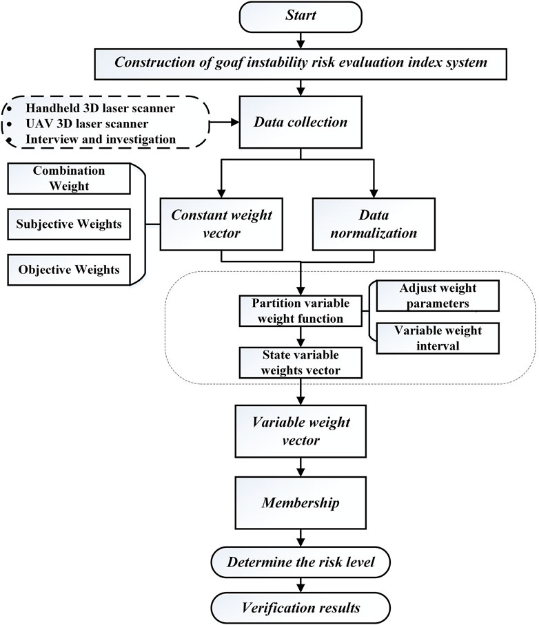
In this study, a comprehensive methodology was employed to assess goaf instability risks. Figure 1 illustrates the research framework. Initially, an evaluation index system tailored to the characteristics of goafs was constructed by selecting 13 key indicators. Data collection involved advanced techniques, such as three-dimensional (3d) laser scanning, unmanned aerial vehicle (UAV) surveys, and field visits. The subjective weights of the evaluation indices were determined using the importance–binary comparison analysis method, and the objective weights were derived using the Gini coefficient weighting method. These weights were then integrated using game theory to form a constant weight model. To enhance the accuracy, we improved this model by incorporating data distribution characteristics into a local variable weight model. Variable weight intervals were established by analyzing the cumulative frequency of the normalized factor indices, and weight-adjustment parameters were determined using the Monte Carlo method. Finally, a cloud model was employed to evaluate the goaf instability risk, providing a robust and precise assessment.

Figure 1

Figure 1. Research framework.

2.1 Data collection and analysis

2.1.1 Study area

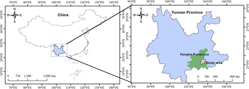
The Bainiuchang Mine is located 42.5 km at a direction of 75° from the downtown area of Mengzi City, Yunnan Province, China (coordinates: 103°45′ to 103°48′, 23°26′30″ to 23°29′30″). The study area (Figure 2), the Baiyang mining area, is located in the northwestern part of the mining area. Mining activities began in 1994, with the peak mining period occurring between 2000 and 2010.

Figure 2

Figure 2. Regional location map of the Bainiuchang mine.

2.1.2 Construction of the evaluation index system for goaf instability risk

Numerous factors contribute to the instability in mined-out areas. Through field surveys and literature review, 13 indicators, including rock mass structure, geological structure, rock quality, ore body dip angle, goaf volume, maximum exposed area, pillar area ratio, ratio of rise to span, embedding depth, exposure time of goaf, mined-out area water, situation of adjacent mined-out areas, and goaf management (Chen et al., 2024; He et al., 2022; Qin et al., 2019; Ren et al., 2022). An evaluation index system for the instability risk in mined-out areas was constructed. Based on the relevant literature and field surveys, the risk levels were identified as I, II, III, and IV, with the risk level classification detailed in Supplementary Table S1 (Guo et al., 2022; Jia et al., 2016; Lang and Chen, 2015). The corresponding standards for each evaluation indicator are listed in Supplementary Table S2 (Hu et al., 2017; Hu, 2022; Ma, 2015; Ren Honggang, 2020; Wang, 2020).

2.1.3 Data collection

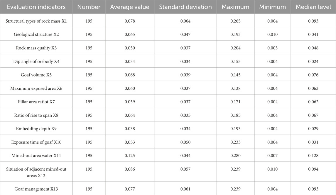
The investigation of the mined-out areas commenced in April 2021 and concluded in October 2022. The team conducted handheld 3D laser scanning surveys of accessible and safe mined-out areas (field surveys and scanning results are shown in Supplementary Figures S1A, C). For areas with high safety risks where direct human entry was not feasible, UAV photography equipment was used for surveying (field survey and scanning results are shown in Supplementary Figures S1B, D). A total of 195 mined-out areas (or groups of mined-out areas) were identified in the Baiyang mining area. Through field surveys and interviews with mining engineering technicians, data on 13 evaluation indicators were collected from 195 mined-out areas in the Baiyang area, as detailed in Table 1.

Table 1

Table 1. Survey data of mined-out area.

The integrity and distribution of data in Table 1 were assessed using violin plots. Owing to space constraints, violin plots for only four indicators (X3, X4, X5, and X6) are presented. Figure 3 shows that under natural conditions, the data patterns in Table 1 generally align with a normal distribution.

Figure 3

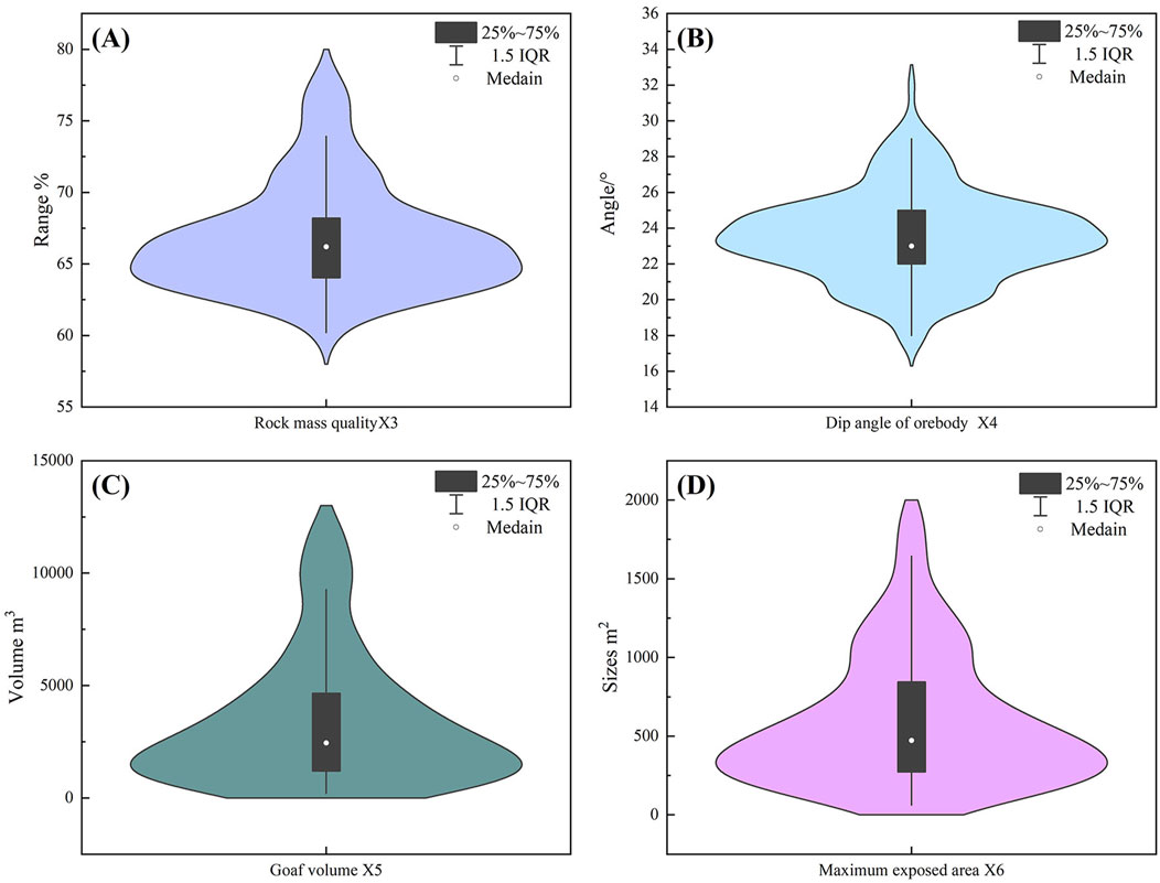
Figure 3. Violin plots with different indexes: (A) Rock mass quality X3; (B) Dip angle of orebody X4; (C) Goaf volume X5; (D) Maximum exposed area X6.

2.2 Determining constant weights

2.2.1 Importance-subjective weight analysis of binary comparison

To reduce the subjectivity of the computational results and simplify the calculation process, this study employs the CRITIC method to comprehensively measure the contrast strength and conflict of the evaluation indicators. This method objectively quantifies the importance for ranking purposes. A preliminary ranking was established and then adjusted based on expert judgment and the initial ranking. Subsequently, a binary comparison method (Wang et al., 2014; Lu et al., 2014) was used to calculate the subjective weights of the indicators without consistency testing. This approach is relatively straightforward and can replace traditional methods such as the AHP to determine the subjective weights of indicators related to the instability risk of mined-out areas.

2.2.1.1 Calculating the importance of evaluation indicators

The dimensionless processing of evaluation indicator values is performed using Equation 1 (Huan-ling et al., 2023; Maneengam, 2023; Qianjun et al., 2023).

$\begin{array}{c}MMS{x}_{ij}^{*}=\frac{x_{ij}-\mathit{min}\left(x_j\right)}{\mathit{max}\left(x_j\right)-\mathit{min}\left(x_j\right)}\\ NMMS{x}_{ij}^{*}=\frac{\mathit{max}\left(x_j\right)-x_{ij}}{\mathit{max}\left(x_j\right)-\mathit{min}\left(x_j\right)}\end{array}(1)$

The standard deviation (Equation 3) is used to represent the difference fluctuation of the internal values of each index to reflect the contrast strength between the evaluation indices, the correlation coefficient (Equation 4) is used to represent the correlation between the indices, and the conflict between the indices is extracted using Equation 5.

$\overline{x_j}=\frac{1}{m}{\displaystyle \sum _{i=1}^m}{x}_{ij}(2)$

$S_j=\sqrt{\frac{1}{m-1}{\displaystyle \sum _{i=1}^m}\left(x_{ij}-\overline{\left.x_j\right)}\right.}(3)$

$r_{ij}=\frac{{\displaystyle {\sum }_{j,k=1}^n}\left(x_{ij}-\overline{x_j}\right)\times \left(x_{ik}-\overline{x_k}\right)}{\sqrt{{\displaystyle {\sum }_{j=1}^n}{\left(x_{ij}-\overline{x_j}\right)}^2\times {\displaystyle {\sum }_{k=1}^n}{\left(x_{ik}-\overline{x_k}\right)}^2}}(4)$

${\eta }_j={\displaystyle \sum _{i=1}^n}\left(1-r_{ij}\right)(5)$

Equations 3, 5 are multiplied to obtain the importance score of the evaluation index.

$C_j=s_j\times {\eta }_j(6)$

2.2.1.2 Importance–binary comparison analysis method

By determining the importance ranking of evaluation indicators using Equations 1–6, the importance of the evaluation indicators for the instability risk of mined-out areas was calculated, and a preliminary importance ranking was established (Wang et al., 2014; Lu et al., 2014). Experts were consulted to make appropriate adjustments to the initial ranking, resulting in a final, practically reflective ranking order.

If the importance of index $u_i$ is not less than that of $u_j$, it is recorded as $u_i\succ u_j$. After sorting, the influencing factors are $u_1^{*},u_2^{*},\cdots ,u_n^{*}$, and the relative importance of each index $u_1,u_2,\cdots ,u_n$ satisfies the relationship is shown in Equation 7:

$u_1^{*}\succ u_2^{*}\succ \cdots \succ u_n^{*}(7)$

2.2.1.3 Selection of scales and calculation of weight coefficients

Based on the ranking of influencing factors, appropriate modal operators and fuzzy membership degrees are selected for each factor from Table 2. The relationship between the scales and membership degrees in Table 2 can be represented by the curve shown in Supplementary Figure S2. When the modal operator falls between two operators in Table 2, interpolation can be used to determine the fuzzy membership degree from Supplementary Figure S2. Finally, a vector matrix is constructed using the fuzzy membership degrees of each factor as weight coefficients, and normalization is applied to obtain the weight vector $B={\left(b_{ij}\right)}_{1\times n}$.

Table 2

Table 2. Mood operator, scale and fuzzy membership.

2.2.2 Objective weighting of Gini coefficient weighting method

The Gini coefficient weighting method is an objective weighting method that calculates the Gini coefficient of the evaluation index and normalizes the Gini coefficient of each index to obtain the weight of the evaluation index. The calculation process is as follows (Dai et al., 2024; Zhao et al., 2024; Li, 2015; Li et al., 2014):

Calculate the Gini coefficient value of the evaluation index:

$G_k=\left\{\begin{array}{cc}{\displaystyle \sum _{i=1}^n}{\displaystyle \sum _{j=1}^n}\left|X_{ki}-X_{kj}\right|/2n^2{\mu }_k& {\mu }_k\ne 0\\ {\displaystyle \sum _{i=1}^n}{\displaystyle \sum _{j=1}^n}\left|X_{ki}-X_{kj}\right|/\left(n^2-n\right)& {\mu }_k=0\end{array}\right.(8)$

where $G_k$ is the Gini coefficient of the k-th index, n is the total number of index data points, and $X_{ki}$ is the i-th value of the k-th evaluation index. ${\mu }_k$ is the expected value of the k-th indicator.

Evaluation index Gini coefficient weight calculation: The Gini coefficient weights of the different indices were obtained by normalizing the Gini coefficient values of each evaluation index.

$g_k=G_k/\left({\displaystyle \sum _{i=1}^m}{G}_i\right)(9)$

2.2.3 Combination weighting based on game theory

The problem of determining the weight of the index combination is solved using game-theory aggregation. Let the weight vector of m indicators calculated by the importance-binary comparative analysis method be ${\overrightarrow{W}}_1^T$, and the weight vector of m indicators obtained by the Gini coefficient objective weighting method be ${\overrightarrow{W}}_2^T$. Let ${\overrightarrow{W}}^T$ be the linear combination of the weight vectors ${\overrightarrow{W}}_1^T$ and ${\overrightarrow{W}}_2^T$. By calculating, the deviation between ${\overrightarrow{W}}^T$ and ${\overrightarrow{W}}_1^T$ and ${\overrightarrow{W}}_2^T$ is minimized, ${\alpha }_p$ can be obtained, and then normalized. The combined weight vector is obtained as follows (Dai et al., 2024; Zhao et al., 2024; Li, 2015; Li et al., 2014):

$\overrightarrow{W}={\displaystyle \sum _{P=1}^2}{\alpha }_P{\overrightarrow{W}}_P^T(10)$

$\min ‖{\displaystyle \sum _{P=1}^2}{\alpha }_P{\stackrel{\rightharpoonup }{W}}_P^T-{\overrightarrow{W}}_l^T‖(11)$

2.3 Determining variable weight

2.3.1 Local variable weight theory

The variable weight theory, introduced by Wang (1985) in the 1980s, posits that the weight of an evaluation indicator dynamically adjusts based on changes in its corresponding state indicator value. Subsequently, Li (1995); Li (1996) provided axiomatic definitions and calculation formulas for three types of variable weights: penalty, incentive, and neutral.

Let the state vector of the evaluation index $x_j$ be $\mathrm{X}=\left(x_1,x_2,\cdots ,x_m\right)$, and let the constant weight vector $W_0=\left(w_1^0,w_2^0,\cdots ,w_m^0\right)$ be obtained using the above combination weighting method. Variable Weight Vector $\mathrm{W}\left(x\right)=\left(w_1\left(x\right),w_2\left(x\right),\cdots ,w_m\left(x\right)\right)$. The variable weight calculation formula (Equation 12), $\mathrm{S}\left(X\right)=\left(S_1\left(X\right),S_2\left(X\right),\cdots ,S_m\left(X\right)\right)$ is the state-variable weight function.

$W\left(X\right)=\frac{W_0•S\left(X\right)}{{\displaystyle {\sum }_{i=1}^m}{w}_i^{\left(0\right)}•S_i\left(X\right)}=\left(\frac{w_1^{\left(0\right)}•S_1\left(X\right)}{{\displaystyle {\sum }_{i=1}^m}{w}_i^{\left(0\right)}•S_i\left(X\right)},\frac{w_2^{\left(0\right)}•S_2\left(X\right)}{{\displaystyle {\sum }_{i=1}^m}{w}_i^{\left(0\right)}•S_i\left(X\right)},\cdots ,\frac{w_m^{\left(0\right)}•S_m\left(X\right)}{{\displaystyle {\sum }_{i=1}^m}{w}_i^{\left(0\right)}•S_i\left(X\right)}\right)(12)$

Duan (2003) proposed a penalty-incentive segmented coordination theorem for state variable weight functions, dividing the penalty phase into initial penalty, strong penalty, and veto stages. Li and Wu (2015); Wu and Li (2016) constructed a four-segment (Equation 13) local variable weight state function based on the variable weight theorems proposed by Li Hongxing et al., further dividing the incentive interval into initial and strong incentive segments.

$S_j\left(x\right)=\left\{\begin{array}{l}{e}^{a_1\left(d_{j1}-x\right)}+c-1\\ c\\ e^{a_2\left(x-d_{j2}\right)}+c-1\\ e^{a_3\left(x-d_{j3}\right)}+e^{a_3\left(d_{j3}-d_{j2}\right)}+c-2\end{array}\right.\begin{array}{c}\begin{array}{c}\left[0,\right.d_{j1})\\ [d_{j1},d_{j2})\end{array}\\ \begin{array}{c}[d_{j2},d_{j3})\\ [d_{j3},1)\end{array}\end{array}(13)$

Among them, c, a₁, a₂, and a₃ are the weighting adjustment parameters, and d_j1, d_j2, and d_j3 are the threshold values for the variable weight intervals of the j-th factor. The variable weight vector is calculated according to Equations 12, 13. Currently, there is no unified method for determining variable weight intervals and variable weight parameters. Li and Wu (2015); Wu and Li (2016) proposed using the K-means method to classify the normalized data of the primary control factors. Then, the threshold values for the variable weight intervals of each factor are determined based on the classification-critical values of various indicators and the calculation formulas. By sequentially constructing evaluation units that meet the constraints and linking them with the constant weight weights to form equations, four weighting adjustment parameters are solved.

However, this method has the following shortcomings (Li and Wu, 2015; Li et al., 2023; Wu and Li, 2016):

1. Clustering analysis results can only indicate data similarity and aggregation degree but cannot reflect the magnitude relationship of the factor state values. The basis for determining interval thresholds through clustering analysis is insufficient.

2. Using the ideal variable weight back-calculation to adjust the parameters is relatively complex in actual calculations, prone to errors, and can sometimes result in unsolvable situations.

3. The state-variable weight functions for different factors are the same; however, their interval thresholds are different, and the factors are independent of each other during the calculation process.

2.3.2 Improved variable weighting model

Based on the characteristics of the variable weight model for evaluating the instability risk of mined-out areas, improvements were made to address its shortcomings.

1. For the local state function, the penalty and incentive intervals in Equation 13 were adjusted. The state function is shown in Equation 14 and illustrated in Supplementary Figure S3.

$S_j\left(x\right)=\left\{\begin{array}{l}{e}^{a_1\left(d_{j1}-x\right)}+e^{a_2\left(d_{j2}-d_{j1}\right)}+c-2\\ e^{a_2\left(d_{j2}-x\right)}+c-1\\ c\\ e^{a_3\left(x-d_{j3}\right)}+c-1\end{array}\right.\begin{array}{c}\begin{array}{c}\left[0,\right.d_{j1})\\ [d_{j1},d_{j2})\end{array}\\ \begin{array}{c}[d_{j2},d_{j3})\\ [d_{j3},1)\end{array}\end{array}(14)$

2. For variable weight intervals, the evaluation indices were divided into qualitative and quantitative indices. For the quantitative indices, the variable weight intervals were determined by analyzing the cumulative frequency of the normalized values for each factor (the division process is shown in Figure 4). For the qualitative indices, variable weight intervals were manually designated. The variable weight intervals at each level were determined using the cumulative frequency of the normalized values of the evaluation indices.

3. Regarding the variable weight intervals, according to the determination method described in Step 2, each evaluation indicator is subdivided into four variable weight interval matrices, denoted as $V_m$. A variable weight matrix I is formed by combining the variable weight intervals of m evaluation indicators. The constant weight vector is multiplied by the variable weight matrix to obtain a comprehensive variable weight interval matrix D.

$Vm=\left(\begin{array}{cccc}\left[0,\right.d_{j1})& [d_{j1},d_{j2})& [d_{j2},d_{j3})& \left[d_{j3},1\right]\end{array}\right)\left(j=1,2,\cdots ,m\right)(15)$

$I=\left(\begin{array}{c}{D}_1\\ D_2\\ ⋮\\ D_m\end{array}\right)=\left(\begin{array}{cccc}\left[0,\right.d_{11})& [d_{11},d_{12})& [d_{12},d_{13})& \left[d_{13},1\right]\\ \left[0,\right.d_{21})& [d_{21},d_{22})& [d_{22},d_{23})& \left[d_{23},1\right]\\ ⋮& ⋮& ⋮& ⋮\\ \left[0,\right.d_{m1})& [d_{m1},d_{m2})& [d_{m2},d_{m3})& \left[d_{m3},1\right]\end{array}\right)(16)$

$\begin{array}{ll}\hfill V=V_m•W_0& =\left(\begin{array}{c}{D}_1\\ D_2\\ ⋮\\ D_m\end{array}\right)•\left(W_0^1,W_0^2,\cdots ,W_0^m\right)\hfill \\ \hfill & =\left(\begin{array}{cccc}\left[0,\right.d_{11})& [d_{11},d_{12})& [d_{12},d_{13})& \left[d_{13},1\right]\\ \left[0,\right.d_{21})& [d_{21},d_{22})& [d_{22},d_{23})& \left[d_{23},1\right]\\ ⋮& ⋮& ⋮& ⋮\\ \left[0,\right.d_{m1})& [d_{m1},d_{m2})& [d_{m2},d_{m3})& \left[d_{m3},1\right]\end{array}\right)\hfill \\ \hfill & •{\left(\begin{array}{c}{W}_0^1\\ W_0^2\\ ⋮\\ W_0^m\end{array}\right)}^T\hfill \end{array}(17)$

4. Based on the determination of the threshold values for the variable weight intervals, it is also necessary to determine the adjustment parameters a₁, a₂, a₃, and c in the model. These parameters can control and adjust the effect of the weight variable. This study attempts to use the Monte Carlo method to trial calculate the adjustment parameters, stipulating the value ranges for a₁, a₂, a₃, and c. Through multiple trial calculations, the accuracy of the evaluation results is maximized, simplifying the calculation process for back-calculating the adjustment parameters and solving the problem of unsolvable calculations.

Figure 4

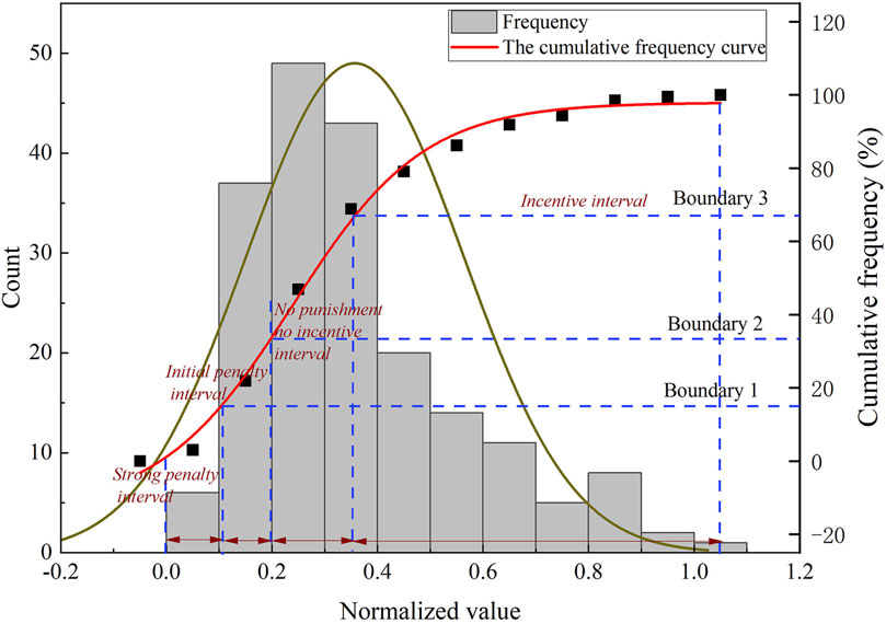
Figure 4. Example of a method for determining variable weighting intervals based on cumula-tive frequency.

2.4 Evaluation of cloud models based on variable weight theory

Using Equations 12, 14, the variable weight vector $\mathrm{W}\left(x_i\right)$ for each goaf is calculated. The cloud model is then used to calculate the membership degree $\mu \left(x_{ik}\right)$ of the goaf instability risk. Based on this, the already obtained variable weight vector $\mathrm{W}\left(x_i\right)$ is multiplied by the membership degrees $\mu \left(x_{ik}\right)$ of the n evaluation indicators for each goaf, resulting in the comprehensive certainty degree $D_k$ of the instability risk of the goaf (Equation 18). The goaf instability risk level is determined based on the maximum membership degree principle. In this study, a forward cloud generator was used to evaluate the goaf instability risk. The calculation steps are shown in Supplementary Figure S4 (Guo L. et al., 2024; Han et al., 2023).

$D_k={\displaystyle \sum _{i=1}^n}\mu \left(x_{ik}\right)•W\left(x_i\right)(18)$

3 Results

3.1 Determination of constant power weights

3.1.1 Importance-binary comparison method to determine the subjective weight

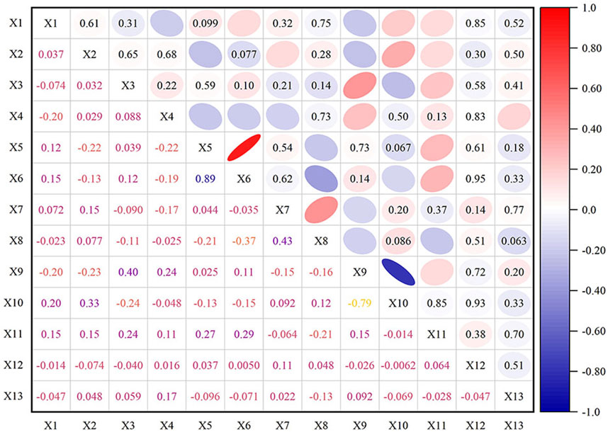
According to Equation 1, the indicators are processed as dimensionless. Using Equations 2, 3, the standard deviation of the evaluation indicators for the goaf instability risk is calculated. Using Equations 4, 5, the correlation coefficients of the evaluation indicators are calculated, and a heat map (Figure 5) is drawn. Using Equation 6, the importance scores of the evaluation indicators are calculated and ranked preliminarily. The results are summarized in Table 3.

Figure 5

Figure 5. Evaluation index correlation coefficient heat map.

Table 3

Table 3. Importance score of evaluation index.

After consulting relevant experts, the preliminary ranking results of the 13 evaluation indicators were adjusted. The adjusted ranking is: X1 $\succ$ X12 $\succ$ X13 $\succ$ X2 $\succ$ X7 $\succ$ X8 $\succ$ X5 = X6 $\succ$ X3 $\succ$ X11 $\succ$ X9 $\succ$ X4 $\succ$ X10. The membership degrees of the factors relative to each other were determined based on the ranking results, as shown in Table 2 and Supplementary Figure S2. The weights of the evaluation indicators were normalized, and the calculation results are listed in Table 4.

Table 4

Table 4. Subjective weight calculation results.

3.1.2 Determine the objective weight

The Gini coefficients of the 13 evaluation indices were calculated using Equation 8 and normalized using Equation 9 to obtain the objective weights of the indices: The calculation results are listed in Table 5.

Table 5

Table 5. The results of objective weight calculation.

3.1.3 Combination weight

According to Equations 10, 11, the combination coefficients of the subjective and objective weights were determined as ${\alpha }_1=0.33,{\alpha }_2=0.79$. After normalization, the weight coefficients were reallocated, resulting in ${{\alpha }_1}^{*}=0.29,{{\alpha }_2}^{*}=0.71$. The combined weights of the 13 evaluation indices that influence the instability risk of the mined-out areas were calculated using Equation 10: The results are as follows: W = (0.0666, 0.0920, 0.0286, 0.0233, 0.0919, 0.1099, 0.0977, 0.0731, 0.1315, 0.1064, 0.1078, 0.0345, 0.0367).

3.2 Calculate the variable weight

3.2.1 Determine the variable weight interval

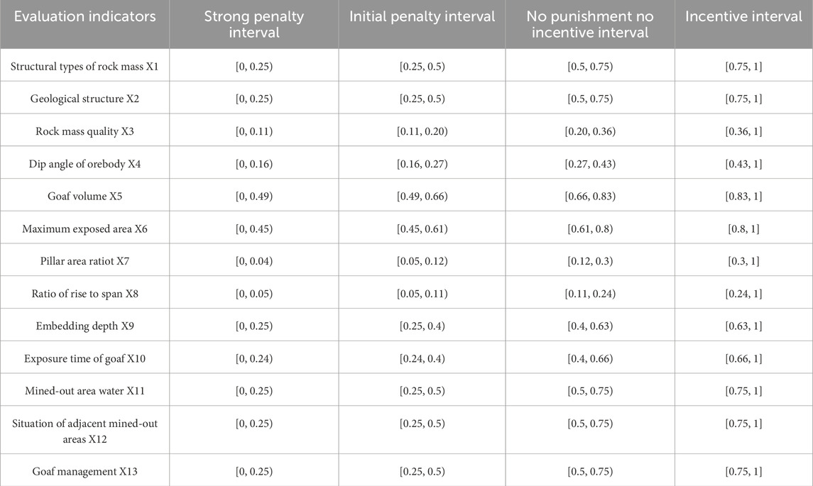
Variable weight intervals were determined using the cumulative frequency of the normalized values of the influencing factors. Owing to the absence of predefined thresholds for categorizing data frequencies as “extreme” or “unique,” this study temporarily defined the cumulative frequency thresholds for state values at 15%, 33%, and 67%. Specifically, the normalized value corresponding to a cumulative frequency of 15% was defined as a strong penalty interval, 33% as an initial penalty interval, and 67% as a neutral interval. The remaining interval was considered the incentive interval. The threshold values for the variable weight intervals were determined by plotting the cumulative frequency intervals of the state values of the main controlling factors (Supplementary Figure S5). Thresholds for factors heavily influenced by human intervention can be manually defined. The final interval thresholds are listed in Table 6.

Table 6

Table 6. Division of evaluation indicators into weighting intervals.

Based on Equations 14–17, the variable weight intervals of the 13 evaluation indices listed in Table 6 were multiplied by constant weights to obtain the comprehensive variable weight interval matrix. The final divisions of the variable weight intervals are listed in Table 7.

Table 7

Table 7. Final variable weight interval classification.

3.2.2 Trial calculations of transfer parameters

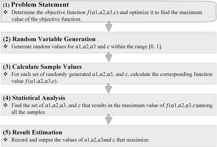
Assuming that the accuracy rate of the instability risk evaluation results for the goaf has a function f (a1, a2, a3, c) related to the adjustment parameters, the Monte Carlo method is used to determine the combination of a1, a2, a3, and c within their ranges to maximize f (a1, a2, a3, c). The specific steps are illustrated in Figure 6.

Figure 6

Figure 6. The calculation process of weight adjustment parameters.

With the aid of MATLAB software, 1,000 assignment tests were conducted to obtain the accuracy rate f (a1, a2, a3, c) of the evaluation results as a function of the adjustment parameters a1, a2, a3, c. The resulting variation curve is shown in Figure 7.

Figure 7

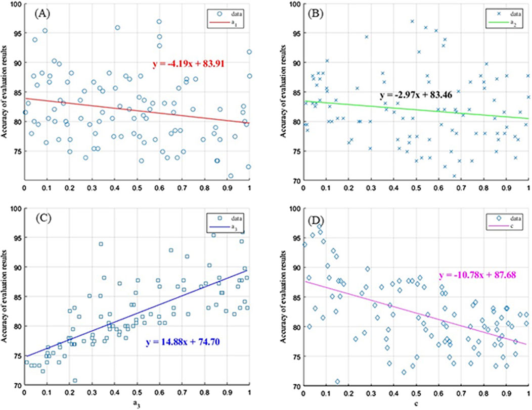
Figure 7. The curve of the change of the weight parameter. (A) The variation curve of the weight adjustment parameter a1; (B) The variation curve of the weight adjustment parameter a2; (C) The variation curve of the weight adjustment parameter a3; (D) The variation curve of the weight adjustment parameter c.

a3 adjusts the amplitude of the weight changes in the incentive interval, a1 and a2 adjust the amplitude of the weight changes in the punishment interval, and c controls the weight adjustments of the entire variable weight model. From Figure 7, it can be concluded that the adjustment parameters a1, a2, and c are negatively correlated with the accuracy of the evaluation results, whereas a3 is positively correlated with the evaluation results. In addition, a1 and a2 have weaker adjustment strengths, whereas a3 and ccc have stronger adjustment strengths. The final adjustment parameters of the variable weight model are listed in Table 8.

Table 8

Table 8. The final value of the weight adjustment parameters.

3.2.3 Variable weight determination

Based on the constructed state variable weight vector formula and the determined variable weight interval and adjustment parameter values, the state variable weight vector Equation 19 for the risk assessment of goaf instability in the Baiyang mine area was established according to Equation 14.

$S_j\left(x\right)=\left\{\begin{array}{ll}{e}^{0.29*\left(0.25-x\right)}+e^{0.66*\left(0.42-0.25\right)}+0.01-2& [0,0.25)\\ e^{0.66*\left(0.42-x\right)}+0.01-1& [0.25,0.42)\\ 0.01& [0.42,0.64)\\ e^{0.67*\left(x-0.64\right)}+0.01-1& [0.64,1)\end{array}\right.(19)$

According to Equation 12, the variable weight value of each evaluation index is calculated, and the relationship between the constant weight and variable weight was drawn (Figure 8). The variable weight data of the 13 evaluation indices were statistically analyzed using Origin software. The results are shown in Table 9.

Figure 8

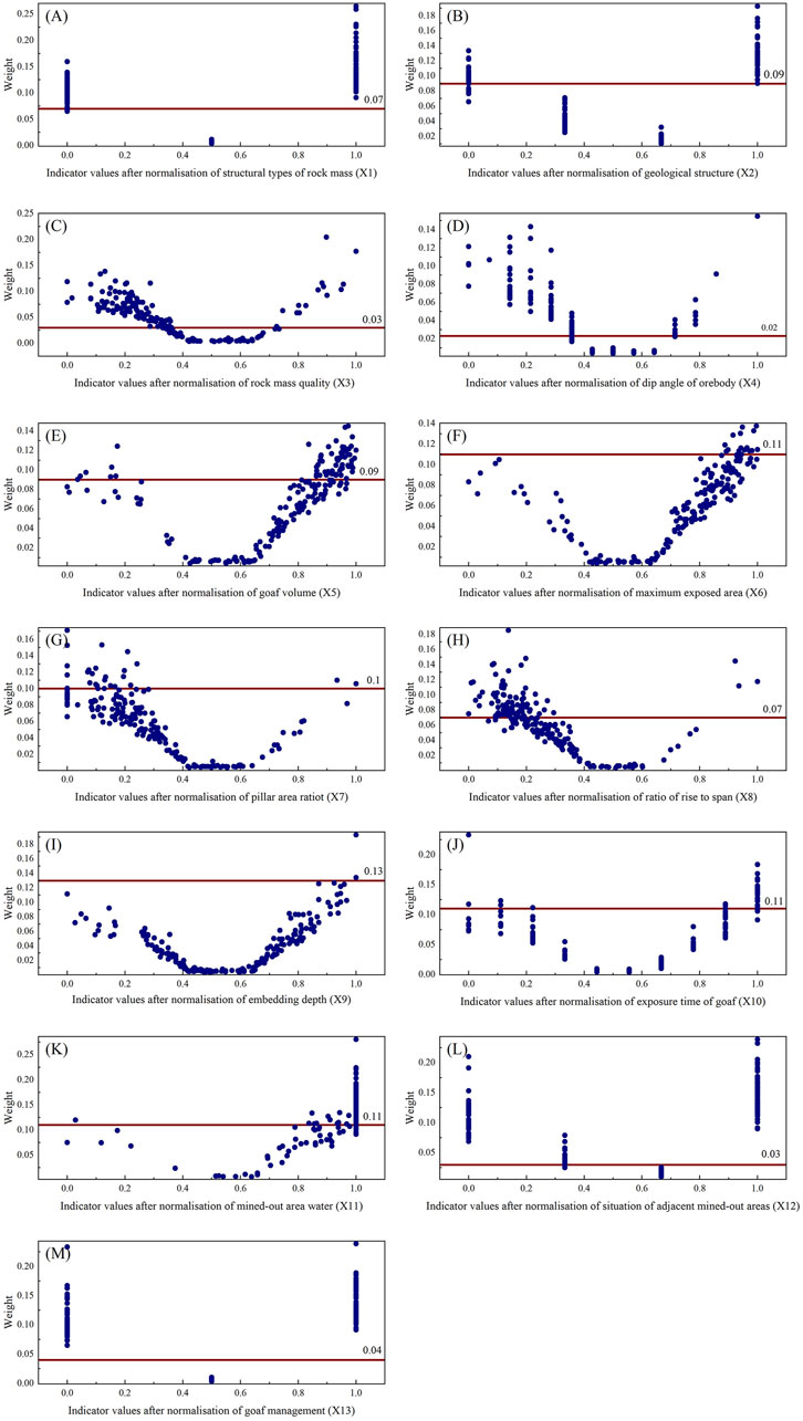
Figure 8. Evaluation index constant weight and variable weight comparison chart. (A) Rock mass structure X1; (B) Geological structure X2; (C) Rock quality X3; (D) Ore body dip angle X4; (E) Goaf volume X5; (F) Maximum exposed area X6; (G) Pillar area ratio X7; (H) Ratio of rise to span X8; (I) Embedding depth X9; (J) Expo-sure time of goaf X10; (K) Mined-out area water X11; (L) Situation of adjacent mined-out areas X12; (M) Goaf management X13.

Table 9

Table 9. Variable weight analysis table.

From the relationship diagram of the constant and variable weight values of the evaluation indicators (Figure 8), it is evident that the constructed variable weight model effectively adjusts the weights of the evaluation indicators during the process of assessing the goaf instability risk in the Baiyang mining area. Specifically, the variable weight model includes the weights of six indicators: rock mass structure (X1), geological structure (X2), rock quality (X3), ore body dip angle (X4), condition of adjacent goafs (X12), and management measures (X13), which significantly increase their weight values. Conversely, the model has “penalized” the weights of seven indicators: goaf volume (X5), maximum exposed area (X6), pillar area ratio (X7), height-span ratio (X8), burial depth (X9), exposure time (X10), and water accumulation in the goaf (X11), reducing their weight values in some goafs.

The average weight of the “neutral” interval (neither penalized nor incentivized) is smaller than that of the other intervals. This is because, under the weight adjustments of the variable weight model, the weights of the factors in the “neutral” interval are compressed. As shown in Table 9, the difference between the average variable and constant weight was not significant. This indicates that the variable weight model not only meets the decision-makers’ preferences for the primary control factors under various combinations of states but also considers the relative importance of the indicator weights. Therefore, in terms of the weight adjustment effects, the constructed variable weight model effectively adjusted the weights of the 13 evaluation indicators according to the predetermined variable weight approach, thus satisfying the expected outcomes.

3.3 Evaluation results of the variable weight model

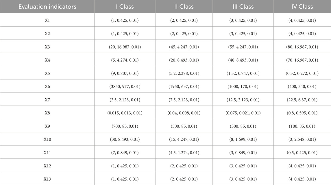
According to the cloud model calculation steps shown in Supplementary Figure S4, the cloud characteristic parameters of the different indicator evaluation standards were calculated, and the results are shown in Table 10. Evaluation grade cloud maps were drawn using MATLAB. Because of space limitations, only a few indicators are shown here in Figure 9.

Table 10

Table 10. Characteristic parameters of each indicator cloud at different levels.

Figure 9

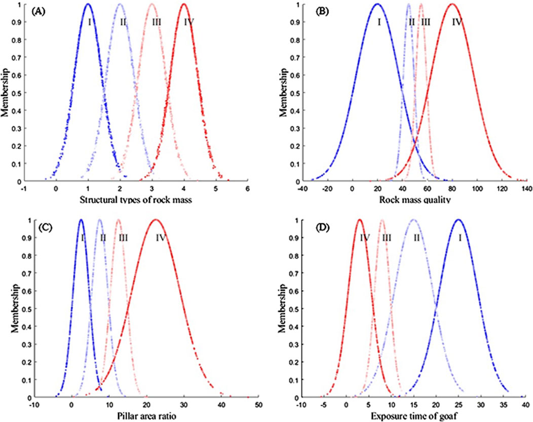
Figure 9. Evaluation grade cloud map of different indicators. (A) Evaluation grade cloud map of structural types of rock mass; (B) Evaluation grade cloud map of rock mass quality; (C) Evaluation grade cloud map of pillar area ratio; (D) Evaluation grade cloud map of exposure time of goaf.

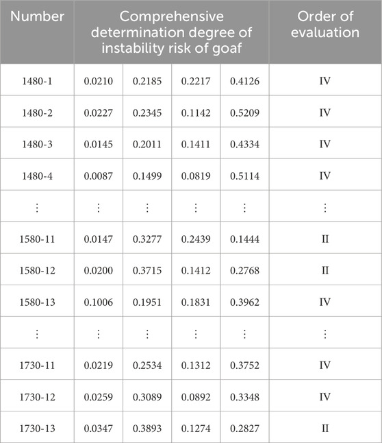
Using Equation 18, the comprehensive determination degree of the instability risk of 195 goafs in the Baiyang mine area was calculated, and the stability grade of the goafs was determined according to the principle of maximum membership degree. The results are shown in Table 11.

Table 11

Table 11. Results of the assessment of the theory of variation.

4 Discussion

4.1 Comparison of evaluation accuracy

Using data from 195 goafs, risk levels were calculated using both variable weight and constant weight models. These results were compared with the actual risk levels to determine the accuracy of the two models. According to Figure 10, the accuracy of risk assessment using the constant weight model was 76.41%, whereas that using the variable weight model was 90.26%. This significant improvement indicates that the variable weight model provides a more accurate assessment of the goaf risk levels than the constant weight model.

Figure 10

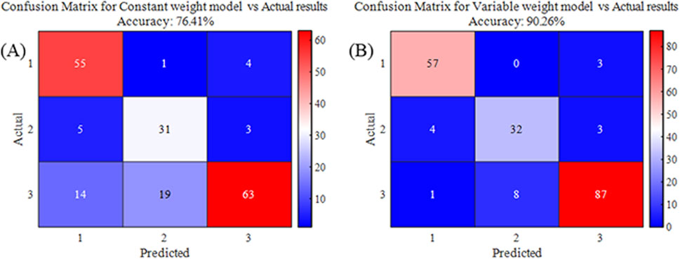
Figure 10. Comparison of results between the two models. (A) Evaluation result accuracy confusion matrix of constant weight model; (B) Evaluation result accuracy confusion matrix of variable weight model.

4.2 Variation in comprehensive determination of goaf instability risk

According to Equation 18, the comprehensive determination of the risk of goaf instability Di in Baiyang Mine under both constant weight and variable weight conditions was calculated for 195 goafs. Di consists of numerical values of four risk levels, as shown in Equation 20. A difference coefficient $\zeta$ was used to measure the discrepancy in the determination of different levels of risk in the goaf (Equation 21). This was compared with the discrepancy in the comprehensive determination of the risk of goaf instability between the constant weight model and the variable weight model (calculated results are shown in Table 12). The bar chart in Figure 11 and the box plot in Figure 12 and illustrate the direct comparison of the distribution of the difference coefficient data for both models.

$D_k=\left[\begin{array}{cccc}I& II& III& IV\\ d_1& d_2& d_3& d_4\end{array}\right](20)$

$\zeta =\frac{\frac{1}{4}\left({\displaystyle \sum _{k=1}^4}\left(d_k-\overline{d_k}\right)\right)}{\overline{d_k}},\overline{d_k}={\displaystyle \sum _{k=1}^4}{d}_k(21)$

Table 12

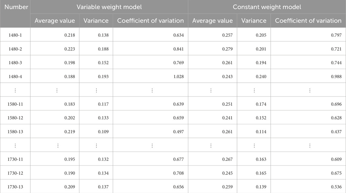
Table 12. The difference of comprehensive determination degree of instability risk in goaf between variable weight model and constant weight model.

Figure 11

Figure 11. Histogram of variation coefficient.

Figure 12

Figure 12. Box plot of coefficient of variation.

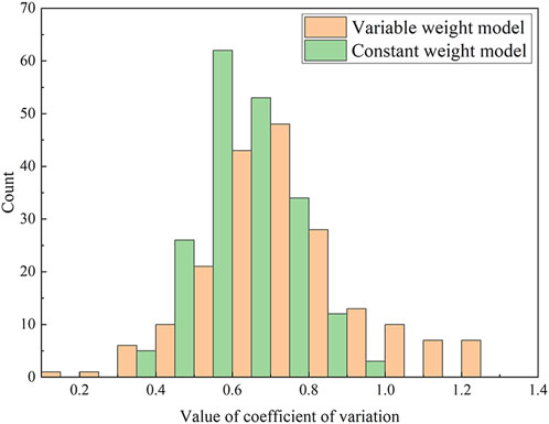
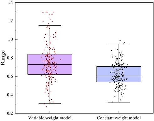
The analysis in Figure 11 shows that the histogram of the variable weight model dataset is higher than that of the constant weight model dataset (approximately 0.75) and the distribution range is wider. The average value of the constant weight model dataset is low and is concentrated near the average value, and the distribution range is narrow. The analysis in Figure 12 shows that the box plot of the variable weight model has a higher median and wider interquartile range (IQR) than the constant weight model. There are more potential outliers in the variable weight dataset, indicating a wider range of values. The results show that the variable weight model has a higher difference coefficient, indicating a wider range of variation in the comprehensive determination. This suggests that the variable weight model better captures the nuances and complexities of the goaf instability risk, providing clearer and more distinguishable membership degrees in the evaluation results.

4.3 Practical significance and future research

These findings enhance the accuracy and reliability of the variable weight model, significantly strengthen mining safety management practices, and ensure safe mining operations. Future research could further refine this assessment framework by incorporating temporal factors and exploring alternative weighting methods. Additionally, extending the application of the variable weight model to other mining environments and geological conditions could provide broader insights into its effectiveness and adaptability.

5 Conclusion

This study employs a systematic approach to construct an index system for evaluating the destabilisation risk of a mining area. The index system is developed based on a comprehensive analysis of the specific characteristics of the mining area in question. In accordance with the tenets of game theory, the subjective and objective weights are integrated and assigned to ascertain the constant weight. Subsequently, in consideration of the characteristics of the indicator values, the local variable weight theory is introduced, and the threshold of the variable weight interval is determined through the normalized cumulative frequency method of the indicators. The Monte Carlo method is employed to determine the adjustment parameters, with the variable weight then applied to each indicator value via the local variable weight state function. The cloud model is subsequently utilised to evaluate the destabilisation risk of the air mining area on this basis. The following main conclusions are drawn in this paper:

1. Although fixed-weight models offer basic assessments, their static weight approaches fail to account for variations and abrupt changes in factor indices. In contrast, the variable weight model dynamically adjusts the weights based on the status values of the influencing factors to overcome this limitation. This flexibility enhances the capability of the model to accurately assess instability risk in mined-out areas, making it a more reliable tool for practical mining safety applications.

2. The variable weight model provided a greater difference in the comprehensive certainty of the goaf instability risk, making the membership degree of the evaluation results clearer and easier to distinguish. This addresses the issue of ambiguity in the results owing to the small differences in membership degrees.

3. In conclusion, the introduction of variable weight theory and the use of the cloud model significantly enhanced the accuracy and reliability of goaf instability risk assessments. Future research can improve the evaluation index system by incorporating time factors and exploring additional weighting methods to refine the model.

Data availability statement

The original contributions presented in the study are included in the article/Supplementary Material, further inquiries can be directed to the corresponding author.

Author contributions

LG: Conceptualization, Data curation, Formal Analysis, Investigation, Methodology, Software, Validation, Visualization, Writing–original draft. KH: Conceptualization, Methodology, Supervision, Validation, Writing–review and editing. HS: Formal Analysis, Software, Writing–review and editing. YY: Investigation, Writing–original draft.

Funding

The author(s) declare that no financial support was received for the research, authorship, and/or publication of this article.

Acknowledgments

The author is grateful to the editor and reviewers for their suggestions. We would like to thank Editage (www.editage.com) for English language editing.

Conflict of interest

The authors declare that the research was conducted in the absence of any commercial or financial relationships that could be construed as a potential conflict of interest.

Publisher’s note

All claims expressed in this article are solely those of the authors and do not necessarily represent those of their affiliated organizations, or those of the publisher, the editors and the reviewers. Any product that may be evaluated in this article, or claim that may be made by its manufacturer, is not guaranteed or endorsed by the publisher.

Supplementary material

The Supplementary Material for this article can be found online at: https://www.frontiersin.org/articles/10.3389/feart.2024.1469834/full#supplementary-material

References

Chen, J., Tan, Y., Huang, X., and Fu, J. (2024). Research on a classification method of goaf stability based on cms measurement and the cloud matter–element model. Appl. Sci. 14, 3774. doi:10.3390/app14093774

CrossRef Full Text | Google Scholar

Dai, R., Xiao, C., Liang, X., Yang, W., Chen, J., Zhang, L., et al. (2024). Spatial-temporal evolution law analysis of resource and environment carrying capacity based on game theory combination weighting and gmd-gra-topsis model. Evidence from 18 cities in henan province, China. J. Clean. Prod. 439, 140820. doi:10.1016/j.jclepro.2024.140820

CrossRef Full Text | Google Scholar

Duan, S. (2003). Variable-weighted comprehensive evaluation method for safety management of electric power enterprises. Math. Pract. Underst. 33, 17–23. doi:10.3969/j.issn.1000-0984.2003.08.004

CrossRef Full Text | Google Scholar

Esmaili, R., and Karipour, S. A. (2024). Comparison of weighting methods of multicriteria decision analysis (mcda) in evaluation of flood hazard index. Nat. Hazards (Dordr) 120, 8619–8638. doi:10.1007/s11069-024-06541-0

CrossRef Full Text | Google Scholar

Fu, Z., Feng, P., and Luo, Z. (2024). Comprehensive assessment of dam safety using a game-theory-based dam safety performance measure. Water (Basel) 16, 659. doi:10.3390/w16050659

CrossRef Full Text | Google Scholar

Guo, D., Meng, F., Wu, H., Yang, X., and Liu, Z. (2024). Risk assessment of shield tunneling crossing building based on variable weight theory and cloud model. Tunn. Undergr. Space Technol. 145, 105593. doi:10.1016/j.tust.2024.105593

CrossRef Full Text | Google Scholar

Guo, L., Hou, K., Sun, H., and Yang, Y. (2024). Stability evaluation of the goaf based on combination weighting and cloud model. Adv. Civ. Eng. 2024, 1–19. doi:10.1155/2024/3884586

CrossRef Full Text | Google Scholar

Guo, W. B., Yang, W. Q., Ma, Z. B., Wen, P., Liu, X., and Bai, E. (2022). Structural stability of overburden structures in mine openings under construction loads and its application. J. Coal Sci. 47, 2207–2217. doi:10.13225/j.cnki.jccs.fq21.1874

CrossRef Full Text | Google Scholar

Han, F., Wang, C., Liu, Z., and Liu, Z. (2023). Assessment of sand accumulation hazard on desert highway based on variable weight-cloud model theory. Front. Earth Sci. (Lausanne) 11. doi:10.3389/feart.2023.1208416

CrossRef Full Text | Google Scholar

He, R., Liu, H., Ren, F., Li, G., Zhang, J., and Zhou, Y. (2022). Comprehensive evaluation and decision for goaf based on fuzzy theory in underground metal mine. Adv. Civ. Eng. 2022. doi:10.1155/2022/3104961

CrossRef Full Text | Google Scholar

Hu, G., Yang, T., Hu, Z., Yu, Q., Zhao, Y., and Zhou, J. (2017). Stability analysis and evaluation of multi-angle mining zone cluster based on mathews stability map and other methods. J. Min. Saf. Eng. 34, 348–354. doi:10.13545/j.cnki.jmse.2017.02.022

CrossRef Full Text | Google Scholar

Hu, J. J. (2022). Destabilization mode and control technology of tungsten mining airspace cluster in Xiangfushan. CNKI. doi:10.26945/d.cnki.gbjku.2022.000151

CrossRef Full Text | Google Scholar

Huan-ling, W., Xu-fei, Z., Hong-jie, C., Kui, Y., Wei-chau, X., and Wei-ya, X. (2023). Evaluation of toppling rock slopes using a composite cloud model with dematel–critic method. Water Sci. Eng. 16, 280–288. doi:10.1016/j.wse.2023.04.002

CrossRef Full Text | Google Scholar

Jia, N., Wu, C., Luo, Z., and Xie, C. (2016). Itopsis and psf coupling for comprehensive identification of the stability of the extraction zone. J. Northeast. Univ. Nat. Sci. Ed. 37, 1182–1187. doi:10.3969/j.issn.1005-3026.2016.08.024

CrossRef Full Text | Google Scholar

Jin, S., Yan, T., Deng, Z., Zhang, W., Liu, Y., Meng, Y., et al. (2024). Evaluation of favorable area for coalbed methane development based on local variable weight theory. Acs Omega 9, 17616–17625. doi:10.1021/acsomega.4c01181

PubMed Abstract | CrossRef Full Text | Google Scholar

Ke, L., Wu, M., Ye, Y., Hu, N., and Meng, Y. (2024). Stability risk early warning for mine goaf: based on d-res and asymmetric fuzzy connection cloud model. J. Comput. Sci. 78, 102279. doi:10.1016/j.jocs.2024.102279

CrossRef Full Text | Google Scholar

Lang, L., and Chen, Z. (2015). Application of fuzzy set-pair analysis in the stability evaluation of mining airspace. J. Central South Univ. Nat. Sci. Ed. 46, 2665–2672. doi:10.11817/j.issn.1672-7207.2015.07.038

CrossRef Full Text | Google Scholar

Li, B., and Wu, Q. (2015). Parameter sensitivity analysis of variable-weight vulnerability evaluation model for coal bed floor water breakout. J. Min. Saf. Eng. 32, 911–917. doi:10.13545/j.cnki.jmse.2015.06.007

CrossRef Full Text | Google Scholar

Li, G. (2015). Research on Gini coefficient assignment method and its application in quality of life evaluation. China Manag. Sci. 23, 193–198.

Google Scholar

Li, G., Cheng, Y. Q., Dong, L. Z., and Wang, W. J. (2014). Research on the objective assignment method of Gini coefficient. Manag. Rev. 26, 12–22. doi:10.14120/j.cnki.cn11-5057/f.2014.01.004

CrossRef Full Text | Google Scholar

Li, H. (1995). Factor space theory and mathematical framework for knowledge representation (viii) - variable weight synthesis principle. Fuzzy Syst. Math., 1–9.

Google Scholar

Li, H. (1996). Factor space theory and mathematical framework for knowledge representation (xi) - construction of equilibrium function and weber-fechner property. Fuzzy Syst. Math., 12–17.

Google Scholar

Li, Z., Ding, X., Liu, S., and Pu, Z. (2023). Vulnerability assessment of bottom slab water breaks based on improved local weighting theory. Coal Sci. Technol. 51, 209–218. doi:10.13199/j.cnki.cst.2021-0959

CrossRef Full Text | Google Scholar

Liu, Y., Eckert, C. M., and Earl, C. (2020). A review of fuzzy ahp methods for decision-making with subjective judgements. Expert Syst. Appl. 161, 113738. doi:10.1016/j.eswa.2020.113738

CrossRef Full Text | Google Scholar

Lu, Y., Linrong, Xu, Chen, S., and Cao, L. (2014). Mudslide hazard evaluation based on game-theoretic combinatorial empowerment. Disaster Sci. 29, 194–200. doi:10.3969/j.issn.1000-811X.2014.01.035

CrossRef Full Text | Google Scholar

Ma, H., Wang, J., and Wang, Y. (2012). Study on mechanics and domino effect of large-scale goaf cave-in. Saf. Sci. 50, 689–694. doi:10.1016/j.ssci.2011.08.050

CrossRef Full Text | Google Scholar

Ma, H. T. (2015). Disaster risk classification and destabilization early warning method for mining airspace area. CNKI.

Google Scholar

Maneengam, A. (2023). Multi-objective optimization of the multimodal routing problem using the adaptive ε-constraint method and modified topsis with the d-critic method. Sustainability 15, 12066. doi:10.3390/su151512066

CrossRef Full Text | Google Scholar

Qianjun, Z., Chuanju, L., Sha, G., Wentong, W., Haoming, L., and Yongheng, J. (2023). Evaluation of the rock burst intensity of a cloud model based on the critic method and the order relation analysis method. Min. Metallurgy and Explor. 40, 1849–1863. doi:10.1007/s42461-023-00838-7

CrossRef Full Text | Google Scholar

Qin, Y., Luo, Z., Wang, J., Ma, S., and Feng, C. (2019). Evaluation of goaf stability based on transfer learning theory of artificial intelligence. Ieee Access 7, 96912–96925. doi:10.1109/access.2019.2929533

CrossRef Full Text | Google Scholar

Ren, L., He, P., Zou, Y., Dun, Z., Zou, Z., and Wang, S. (2022). A new classification method of mine goaf ground activation considering high-speed railway influence. Front. Earth Sci. (Lausanne) 10. doi:10.3389/feart.2022.896459

CrossRef Full Text | Google Scholar

Ren Honggang (2020). Research on multifactor impact analysis and optimization technology of yichang phosphate mining. CNKI. doi:10.26945/d.cnki.gbjku.2020.000092

CrossRef Full Text | Google Scholar

Wang, L., Guo, Q., and Yu, X. (2023). Stability-level evaluation of the construction site above the goaf based on combination weighting and cloud model. Sustainability 15, 7222. doi:10.3390/su15097222

CrossRef Full Text | Google Scholar

Wang, P. (1985). Fuzzy sets and random sets in shadow. Beijing China: Beijing Normal University Press.

Google Scholar

Wang, W., Li, W., Qu, F., Dong, T., Wang, G., Wu, L., et al. (2024). An improved grey relational theory evaluation method: considering the comprehensive performance of autonomous vehicles in virtual test. Int. J. Automot. Technol. 25, 1235–1249. doi:10.1007/s12239-024-00113-8

CrossRef Full Text | Google Scholar

Wang, W., Xu, D., Chau, K., and Lei, G. (2014). Assessment of river water quality based on theory of variable fuzzy sets and fuzzy binary comparison method. Water Resour. Manag. 28, 4183–4200. doi:10.1007/s11269-014-0738-4

CrossRef Full Text | Google Scholar

Wang, Z. (2020). Research on regional hazard prediction technology of roof fall in underground metal mines. CNKI. doi:10.27493/d.cnki.gzdzy.2020.001724

CrossRef Full Text | Google Scholar

Wu, Q., and Li, Bo (2016). Method for determining variable weight interval and tuning parameter in variable weight evaluation of coal bed bottom water breakout. J. Coal 41, 2143–2149. doi:10.13225/j.cnki.jccs.2015.1197

CrossRef Full Text | Google Scholar

Yao, B., Wang, L., Gao, H., and Ren, L. (2024). Bridge construction risk assessment based on variable weight theory and cloud model. Buildings-Basel 14, 576. doi:10.3390/buildings14030576

CrossRef Full Text | Google Scholar

Zhang, Q., Wang, C., Han, L., Hao, J., Qiao, L., and Chen, S. (2023). Study on stability analysis and treatment of underground goaf in metal mine. Min. Metallurgy and Explor. 40, 1973–1985. doi:10.1007/s42461-023-00764-8

CrossRef Full Text | Google Scholar

Zhang, Y., and Shang, K. (2024). Evaluation of mine ecological environment based on fuzzy hierarchical analysis and grey relational degree. Environ. Res. 257, 119370. doi:10.1016/j.envres.2024.119370

PubMed Abstract | CrossRef Full Text | Google Scholar

Zhang, Y., Zhao, H., Fu, C., and Tie, Y. (2024). Optimal placement of structural sensors in complex service environments using data relational analysis. Mech. Syst. Signal Process 217, 111523. doi:10.1016/j.ymssp.2024.111523

CrossRef Full Text | Google Scholar

Zhao, B., Shao, Y. B., Yang, C., and Zhao, C. (2024). The application of the game theory combination weighting-normal cloud model to the quality evaluation of surrounding rocks. Front. Earth Sci. (Lausanne) 12. doi:10.3389/feart.2024.1346536

CrossRef Full Text | Google Scholar

Zhe, Y., Hou, K., Niu, X., and Liang, W. (2023). Early warning technique research of surface subsidence for safe mining in underground goaf in karst plateau zone. Front. Earth Sci. (Lausanne) 11. doi:10.3389/feart.2023.1266649

CrossRef Full Text | Google Scholar

Zheng, W., Xu, S., and Wang, Z. (2024). Fuzzy comprehensive evaluation of collapse risk in mountain tunnels based on game theory. Appl. Sci. 14, 5163. doi:10.3390/app14125163

CrossRef Full Text | Google Scholar