A study on groundwater level calculation based on PCA-CIWOABP

In order to explore the relationship between groundwater levels and hydro-meteorological factors in Fengnan District, accurate estimation of groundwater levels in the area was undertaken. Real data on groundwater levels, water consumption, and rainfall from 2018 to 2021 in various townships within Fengnan District were selected. Utilizing the Principal Component Analysis method, the main influencing factors were extracted from the hydrological data of each township. Subsequently, a groundwater level calculation model was established using the CIWOABP(Cubic map - Intelligent weight adjustment - Whale Optimization Algorithm–Back Propagation) neural network in combination with these factors. The results indicate that: (1) Principal Component Analysis extracted a total of five principal components from various hydrological data in Fengnan District, namely, groundwater levels of monitoring wells #11 and #12, rainfall from rainfall station r1, and water consumption from Fengnan (FN) and Qianying (QY) towns. (2) The CIWOABP neural network was trained using 36 sets of actual measurement data and validated with 12 sets of simulated data. The mean absolute errors (MAE) for monitoring wells #11 and #12 were 0.19 and 0.23 respectively, and the mean squared errors (MSE) were 0.05 and 0.09 respectively. The model exhibited high computational accuracy and can be effectively employed to calculate actual groundwater levels. The research outcomes can provide theoretical and methodological insights for groundwater resource management in the North China Plain.

1 Introduction

Groundwater resources play an irreplaceable role in various sectors such as production, daily life, and ecological environments (Chai et al., 2023; Stigter et al., 2023). However, persistent overexploitation and improper utilization of groundwater have led to various issues, including continual decline in groundwater levels (Costa et al., 2021) and deterioration of water quality (Hou et al., 2023). These problems pose threats to the sustainable utilization of water resources and ecological balance. Effectively addressing these potential risks necessitates the accurate prediction of groundwater level fluctuations, a challenging task. Groundwater level prediction is often hindered by issues such as high-dimensional data, model complexity, and computational costs, posing significant challenges in practical applications (Zaghiyan et al., 2021). Therefore, the quest for a more efficient and precise groundwater level prediction method becomes especially crucial.

Subject to the comprehensive influences of various factors including rainfall, soil type, evapotranspiration, groundwater extraction, recharge, seasonal and climatic variations, land cover, and groundwater flow, the simulation and prediction of groundwater levels face substantial hindrances (Li et al., 2013; Deb, 2024). In order to mitigate the adverse impact of these complex factors on the simulation and prediction of groundwater level fluctuations, some researchers have employed the Principal Component Analysis (PCA) method to address the intricate relationships among influencing factors of groundwater levels. This approach involves dimensionality reduction to enhance the accuracy and stability of predictive models. Generally, there are two approaches to dimensionality reduction of original data concerning groundwater levels and their influencing factors using PCA: The first approach involves employing PCA to extract primary components from a multitude of factors that contribute to fluctuations in groundwater levels (Almanaseer and Sankarasubramanian, 2012; Chang et al., 2017). Jung et al. (2021) utilized Principal Component Analysis to perform dimensionality reduction on observed data including rainfall, evaporation, groundwater usage, tides, and more. Subsequently, they identified rainfall as a primary component, leading to a notable reduction in subsequent monitoring costs. The second approach involves Principal Component Analysis to extract composite data from a single factor that represents the original dataset (Naderianfar et al., 2017; Kim et al., 2021). Triki et al. (2014) applied Principal Component Analysis and cluster analysis to actual groundwater level data from 24 monitoring wells, categorizing them into three distinct groundwater fluctuation patterns. They further analyzed how these different patterns responded to variations in rainfall and temperature.

When dealing with accurate simulation and prediction of groundwater levels, traditional hydraulic calculations and big data-driven neural networks emerge as two primary methodologies. Traditional approaches build mathematical models for groundwater flow based on hydraulic motion equations. However, the complexity of groundwater systems and difficulties in data acquisition restrict their applicability and predictive capability (Matiatos et al., 2019; Li X. Q. et al., 2022). In recent years, neural network technology has emerged as a promising avenue for groundwater level prediction, offering new perspectives. Neural network types such as Convolutional Neural Networks (CNN), Recurrent Neural Networks (RNN), and Long Short-Term Memory Networks (LSTM) have been widely applied in groundwater level modeling. They can capture nonlinear relationships, enhancing model accuracy and generalization (Bowes et al., 2019; Xu et al., 2022; Yang and Zhang, 2022). Among these, the Backpropagation Neural Network (BPNN) stands out for its adaptability and generalization capabilities. BP neural networks adjust weights across multiple layers of neurons, learning groundwater level variation patterns from input data to achieve precise predictions (Zhang et al., 2022). Moreover, the incorporation of optimization algorithms further enhances the performance of the BP neural network. These algorithms adjust weights and biases to reduce prediction errors. Optimization techniques such as Artificial Bee Colony, Ant Colony, and Wavelet Decomposition have been introduced to improve model convergence speed, computational accuracy, and stability, resulting in improved predictive capabilities (Dash et al., 2010; Hosseini et al., 2016; Li et al., 2019; Zhang, 2022; Serravalle Reis Rodrigues et al., 2023).

The reviewed studies present advanced methodologies leveraging the Whale Optimization Algorithm (WOA) for improving water resource management. Notably, (Wang et al., 2023) introduces a robust monthly runoff interval prediction model combining WOA, Variational Modal Decomposition (VMD), LSTM networks, and non-parametric kernel density estimation. This innovative approach addresses the limitations of traditional point prediction by effectively capturing prediction uncertainty, thus aiding water management decisions. Other studies demonstrate the application of enhanced WOA variants in diverse contexts. For example, a multi-level scheduling method for mine water reuse utilizes opposition-based learning, Levy flight, nonlinear convergence factors, and adaptive inertia weight to enhance convergence speed, accuracy, and efficiency, significantly boosting reuse efficiency (Bo et al., 2022). Another study focuses on optimizing water resource allocation in Handan, China, using an ameliorative WOA with logistic mapping and inertia weighting, leading to more reliable water usage predictions (Yan et al., 2018). Further, an enhanced WOA for clustering incorporates elements from water wave optimization and tabu search, achieving superior performance compared to existing algorithms (Singh et al., 2023). Finally, the application of WOA and its enhancement at the Klang Gate Dam for reservoir operation optimization shows significant improvements in reducing water deficits and increasing reliability (Lai et al., 2021). Collectively, these studies highlight the versatility and efficacy of WOA and its variants in addressing complex water management challenges, providing valuable insights and tools for decision-makers.

In conclusion, the fluctuation of groundwater levels is influenced by complex factors, and traditional hydraulic calculation methods struggle to comprehensively account for various changing elements compared to neural network models. Therefore, this study aims to explore and enhance groundwater level prediction methods by combining principal component analysis for dimensionality reduction with an optimized BP neural network model. This approach seeks to elevate the accuracy and stability of groundwater level simulation.

2 Materials

2.1 Research area

The North China Plain is the world’s largest area of groundwater funneling, with the majority of groundwater funnel zones concentrated in Hebei Province. Currently, over 20 groundwater funnel zones have merged into a vast interconnected area within Hebei Province, forming a super-sized groundwater funneling region. The study area (Fengnan District) is located in the eastern coastal plain of Hebei Province, in the southern part of Tangshan City, situated between 117°51′43″E and 118°25′28″E longitude, and 39°11′59″N and 39°39′28″N latitude. The study area is bordered to the north by Fengrun District and Lutunan District of Tangshan City, to the south by the Bohai Sea, and is adjacent to Kaiping District, Luan Nan County, and Caofeidian New Area of Tangshan City to the east. To the west, it adjoins Binhai New Area and Ninghe District of Tianjin Municipality. Within the study area, there are two fifth-level rivers, Tang River and Sha River, and adjacent to it, there are two other rivers, Ning River and Luan River. The study area spans approximately 50 km from north to south and 48 km from east to west, covering a total area of 1288.4 square kilometers. The distribution of groundwater monitoring wells within Fengnan District and its surroundings is illustrated in Figure 1.

Figure 1

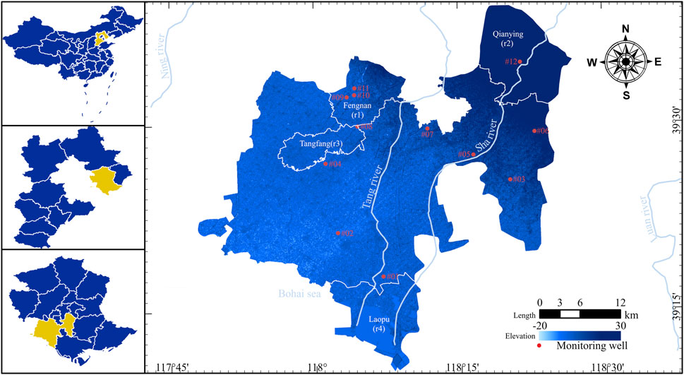
Figure 1. Map of research area. Created by ArcGIS 10.6 software (https://www.arcgis.com).

2.2 Data source

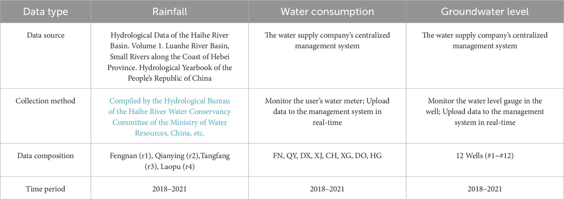
In the study area, the groundwater level experiences fluctuation due to both anthropogenic factors such as domestic and industrial water consumption, and natural factors including rainfall and infiltration. Currently, we have obtained water consumption data for major townships within the region from 2018 to 2021, rainfall data from rainfall stations, and groundwater level data from 12 monitoring wells. Detailed data information can be found in Table 1.

Table 1

Table 1. Data attributes.

3 Methods

3.1 Combined PCA and CIWOABP neural network structures

The empirical dataset of this study exhibits the following characteristics: a relatively small variety of factors influencing groundwater level fluctuations, longer time series for the data records, but a relatively smaller number of data instances; within the same factor, multiple data categories are present, including 12 types of monitoring wells for groundwater levels, four rainfall stations for rainfall, and eight townships for water consumption. If the raw dataset is directly employed for training and prediction using the BP neural network, it is difficult to achieve highly desirable results.

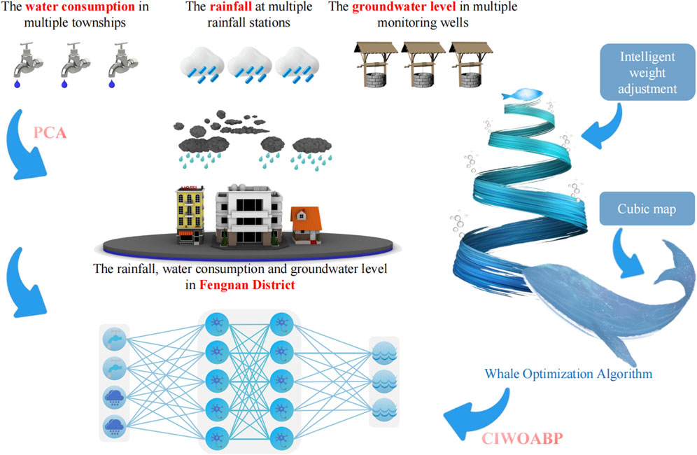
Therefore, Dimensionality reduction was performed on water consumption, rainfall, and groundwater level data based on PCA. This process involved selecting mutually complementary townships, rainfall stations, and monitoring wells, as well as eliminating collinearity among variables. Principal components with cumulative variance contribution rates ranging from 85% to 100%, or eigenvalues greater than 1, were chosen as input and output data for the CIWOABP neural network (Wold et al., 1987; Jolliffe, 2022). Ultimately, a fitting study of the groundwater level calculation model for the Fengnan area was conducted. The technical roadmap of the study is illustrated in Figure 2.

Figure 2

Figure 2. Technical flow chart.

3.2 Principal component analysis

The PCA method finds widespread application in data dimensionality reduction and denoising. PCA achieves this by linear transformation, converting high-dimensional data into a lower-dimensional space where the components are relatively independent. This approach maximizes the retention of essential key information from the original dataset, thereby achieving dimensionality reduction. The calculation steps of PCA are as follows (Demšar et al., 2013; Lin et al., 2022; Marukatat, 2023):

The formula for calculating the covariance matrix is as Equation 1:

$C=\frac{1}{m}{\sum }_{i=1}^m\left(x_i-\mu \right){\left(x_i-\mu \right)}^T(1)$

where $C$ represents the covariance matrix, $m$ is the number of samples, $x_i$ denotes the original data, and $\mu$ is the mean vector of the data.

The formula for eigenvalue decomposition is as Equation 2:

$C=PD{P}^{-1}(2)$

where P is a matrix composed of eigenvectors, and D is a diagonal matrix consisting of eigenvalues arranged on the diagonal.

Selecting the eigenvectors corresponding to the k largest eigenvalues as principal components, the dimension-reduced data can be calculated using Equation 3:

$\overline{y}=\overline{x}\left(\overline{v_1}\overline{v_2}\cdots \overline{v_k}\right)(3)$

where $\overline{y}$ represents the data after dimensionality reduction, $\overline{x}$ is the data after subtracting the mean from the original data, and $\overline{v_i}$ represents the eigenvector of the ith principal component.

4 CIWOABP neural network

4.1 Whale optimization algorithm

In nature, whales form social groups and seek food based on interactions and foraging behaviors among individuals. Whales adjust their behavior to find more food by responding to changes in their surroundings and their own perception of the environment. The WOA applies this foraging strategy, treating the problem-solving process as a search for food (i.e., optimal solutions) in the solution space. In Figure 2, the basic structure of the BP neural network is 'input layer - neurons - output layer’, which involves forward propagation calculation and backward feedback adjustment of weights and biases to optimize the solution. The whale optimization algorithm combines global and local search strategies to optimize the weights and biases of the BP neural network, thereby improving the performance and convergence speed of the neural network (Mirjalili and Lewis, 2016).

In the WOA, the current optimal individual is assumed to be the prey, while other individuals converge towards the optimal one. The mathematical model of this process is represented as follows:

$\mathit{X}\left(t_{i+1}\right)={\mathit{X}}_{\mathit{p}}\left(t_i\right)-\mathit{A}\cdot \left|\mathit{B}\cdot {\mathit{X}}_{\mathit{p}}\left(t_i\right)-\mathit{X}\left(t_i\right)\right|(4)$

where $\mathit{X}$ is the individual’s position vector, $t_i$ represents the ith iteration or evolution count, ${\mathit{X}}_{\mathit{p}}$ denotes the prey’s position vector, and $\mathit{A}$ and $\mathit{B}$ are coefficient vectors, which can be defined as:

$\mathit{A}=2a{r}_1-a(5)$

$\mathit{B}=2r_2(6)$

where $r_1$ and $r_2$ are random numbers within the range [0, 1], a is known as the convergence factor, which linearly decreases from 2 to 0 as the iteration count increases, i.e.,:

$a\left(t_i\right)=2-\frac{2t_i}{t_{\mathit{max}}}(7)$

where $t_{\mathit{max}}$ represents the maximum number of iteration evolutions.

To mathematically describe the bubble-net feeding behavior of whales, this study incorporates two distinct approaches within the WOA algorithm: the Converging Encircling Mechanism and the Spiral Updating Position. The Converging Encircling Mechanism is implemented through Equations (4–7) as the convergence factor 'a' diminishes. In the Spiral Updating Position method, the simulated spiral motion of whales is employed to capture prey, and its mathematical model is represented as Equation 8:

$\mathit{X}\left(t_{i+1}\right)={\mathit{D}}^{\prime }\cdot e^{bl}\cdot \cos \left(2\pi l\right)+{\mathit{X}}_{\mathit{p}}\left(t_i\right)(8)$

where ${\mathit{D}}^{\prime }=\left|{\mathit{X}}_{\mathit{p}}\left(t_i\right)-\mathit{X}\left(t_i\right)\right|$ represents the distance between the current individual and the prey, b is a constant, and l is a random number within the range [-1, 1].

In addition to the bubble-net feeding behavior, whales can also search for food randomly. When $\left|\mathit{A}\right|>1$, individual whales perform random searches based on their positions relative to each other. The mathematical model for this is:

$\mathit{X}\left(t_{i+1}\right)={\mathit{X}}_{\mathit{r}\mathit{a}\mathit{n}\mathit{d}}\left(t_i\right)-\mathit{A}\cdot \left|\mathit{C}\cdot {\mathit{X}}_{\mathit{r}\mathit{a}\mathit{n}\mathit{d}}\left(t_i\right)-\mathit{X}\left(t_i\right)\right|(9)$

where ${\mathit{X}}_{\mathit{r}\mathit{a}\mathit{n}\mathit{d}}$ represents the position vector of a randomly selected whale individual from the current population.

4.2 Cubic map

The initial whale population generated by random methods is unevenly distributed in the solution space, with poor diversity, which cannot effectively extract useful information from the solution space, thus affecting the search efficiency of the algorithm to some extent. Cubic mapping can be used to replace pseudo-random number generators, i.e., generating chaotic numbers between 0 and 1. Previous research has shown that using chaotic sequences for population initialization often yields better results (Wang et al., 2014; Kaur and Arora, 2018).

In this study, the Cubic map is employed to optimize the random approach for initializing the population in the WOA, with the following Equation 10:

$z_{k+1}=c\left(1-z_k^2\right)(10)$

where $z_k$ represents the iteration value of the kth generation, and c is the adjusting coefficient.

4.3 Intelligent weight adjustment

From the previous Equation 7, it can be observed that in the basic WOA algorithm, the value of the control parameter “a” linearly decreases from 2 to 0 as the number of iterations increases. In fact, the optimization process of the WOA algorithm is highly complex, and the linear decrease strategy of the control parameter “a” cannot adapt well to the actual optimization process. It can easily lead to low convergence accuracy or getting stuck in local optima (Li M. et al., 2022). This study employs an adaptive algorithm to modify the weight values of the whale population during each evolution process, as Equation 11:

$w=w_{\mathit{min}}+m\left(w_{\mathit{max}}-w_{\mathit{min}}\right)e^{\frac{-t_i}{t_{\mathit{max}}}}(11)$

where w is the weight coefficient, $w_{\mathit{min}}$ and $w_{\mathit{max}}$ are the initial and final values of the weight coefficient, and m is the adjustment coefficient.

4.4 Model evaluation

To validate the predictive results of the PCA-CIWOABP coupled model for groundwater levels in the Fengnan area, this study employs the following six evaluation metrics as quantitative assessment criteria for evaluating the prediction results: Mean Absolute Error (MAE), Mean Squared Error (MSE), Root Mean Squared Error (RMSE), Mean Absolute Percentage Error (MAPE), Nash efficiency coefficient (NSE) and Pearson correlation coefficient (R), with the calculation formulas as Equations 12–17 (Zhang et al., 2023; Zhang et al., 2024a; Zhang et al., 2024b):

$MAE={\sum }_{i=1}^n\left|h_i-f_i\right|/n(12)$

$MSE={\sum }_{i=1}^n{\left(h_i-f_i\right)}^2/n(13)$

$RMSE={\sum }_{i=1}^n{\left({\left(h_i-f_i\right)}^2/n\right)}^{1/2}(14)$

$MAPE={\sum }_{i=1}^n\left|\left(h_i-f_i\right)/f_i\right|/n*100\%(15)$

$NSE=1-{\sum }_{i=1}^n{\left(h_i-f_i\right)}^2/{\sum }_{i=1}^n{\left(h_i-\overline{h}\right)}^2(16)$

$R={\sum }_{i=1}^n\left(h_i-\overline{h}\right)\left(f_i-\overline{f}\right)/\left[\sqrt{{\sum }_{i=1}^n{\left(h_i-\overline{h}\right)}^2}\sqrt{{\sum }_{i=1}^n{\left(f_i-\overline{f}\right)}^2}\right](17)$

where $h_i$ represents the actual measured values, $f_i$ represents the predicted values, $\overline{h}$ and $\overline{f}$ are the average values of their respective datasets, and n denotes the number of data samples.

5 Result and discussion

5.1 Fluctuations in the distribution of groundwater levels

In this study, the fluctuation of groundwater level is primarily associated with residential water consumption and rainfall, while the distribution of groundwater level is correlated with the local water systems and elevation. Based on the annual average groundwater levels of monitoring wells within the region from 2018 to 2021, a contour map of groundwater levels was generated using the inverse distance weighted interpolation method, as shown in Figure 3.

Figure 3

Figure 3. Distribution of annual average groundwater levels: (A) 2018, (B) 2019, (C) 2020, and (D) 2021.

To further investigate the seasonal fluctuation of groundwater levels within the Fengnan area, this study took monitoring wells #01, #05, #07, and #12 as examples and plotted the water level variations for each month. The specific results are depicted in Figure 4.

Figure 4

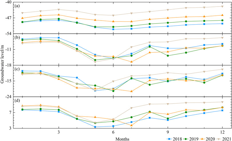
Figure 4. Fluctuations in monthly average groundwater levels: (A) #01, (B) #05, (C) #07, and (D) #12.

The groundwater levels at various monitoring wells exhibit a trend of “initial decrease followed by an increase,” with the lowest levels typically occurring between May and July. Among them, the lowest water levels for each monitoring well were generally observed in May for the years 2018, 2019, and 2021. However, in 2020, the groundwater levels at all locations reached their nadir in July. For instance, monitoring well #12 reached its lowest levels in July 2020 and May 2021, with levels of 3.73 m and 4.45 m respectively.

The fluctuation of groundwater levels is not only influenced by local government water management measures but also related to the replenishment from nearby water systems. Combining with Figure 1, it can be observed that monitoring well #01 is located near the downstream of the Tang River, monitoring well #05 and #12 are situated in the middle and upper reaches of the Sha River respectively, and monitoring well #07 is positioned between the Tang River and the Sha River, receiving minimal replenishment from the river systems. Additionally, monitoring well #01 is closer to the Bohai Sea compared to other monitoring wells, and the rivers in Figure 1 all belong to the fifth-level river system, indicating relatively weak influence of river systems on groundwater levels. Therefore, monitoring well #01 steadily increased from 2018 to 2021, with a water level difference of 7.02 m between the beginning of 2018 and the end of 2021; monitoring well #05, #07, and #12 did not show significant changes in water levels compared to monitoring well #01, with differences in groundwater levels at the beginning and end of 2018 and 2021 being less than 1 m for monitoring well #05 and #07.

5.2 Principal component analysis results

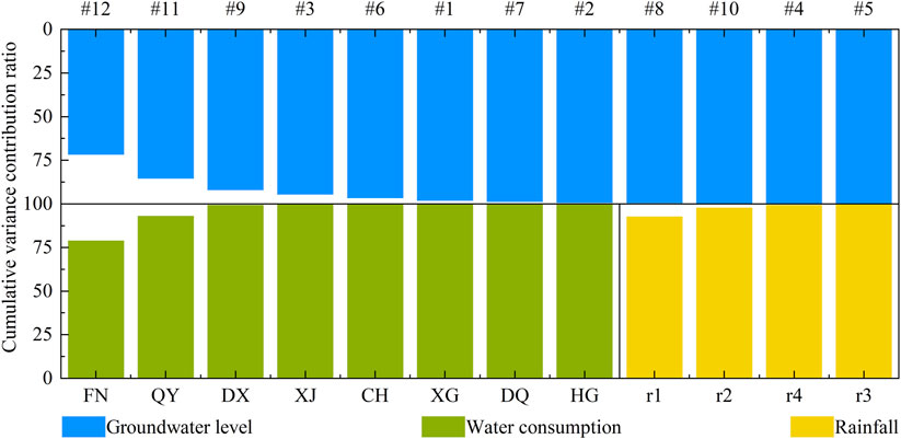
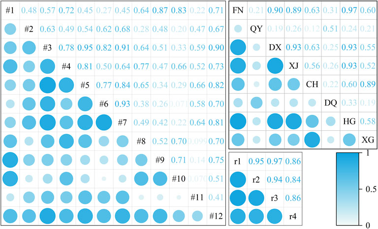
In this study, due to the existence of multiple indicator factors for rainfall, water consumption, and groundwater levels, directly constructing a neural network would require a substantial amount of measured data. Consequently, the raw data was first standardized and then subjected to PCA using SPSS. The cumulative contribution rates and correlation coefficients of each component are illustrated in Figures 5, 6, respectively. In order to reduce data dimensionality, enhance data interpretability, filter out data noise, and prevent overfitting, this paper not only ranked and accumulated the variance contribution rates of each component one by one but also regarded components with cumulative variance contribution rates greater than 85% as the principal components of their respective datasets.

Figure 5

Figure 5. Cumulative variance contribution ratio.

Figure 6

Figure 6. Correlation coefficient.

As shown in Figure 5, for groundwater levels, the variance contribution rates of monitoring wells #11 and #12 are 71.74% and 13.77%, respectively, with a cumulative contribution rate exceeding 85%. Hence, these two monitoring wells can be extracted as principal components and denoted as $G_1$ and $G_2$. Concerning residential water usage, the variance contribution rates for towns FN and QY are 78.78% and 14.23%, respectively, resulting in a cumulative contribution rate exceeding 90%. Therefore, these two towns can be extracted as principal components and labeled as $W_1$ and $W_2$. For rainfall, only rainfall station r1 achieves a contribution rate of 92.80%, leading to a cumulative contribution rate exceeding 90%. Thus, this rainfall station can be extracted as a principal component and denoted as $R_1$.

Considering the correlation coefficients in Figure 6, it's evident that the larger the absolute value of correlation coefficient between components, the closer the relationship between the original variables and that principal component. For groundwater levels, the first principal component $G_1$ shows higher correlation coefficients with monitoring wells #3 to #7, while the second principal component $G_2$ demonstrates higher correlations with monitoring wells #1 to #10, all exceeding 0.5. The linear combinations expressing the relationships between each principal component and the original variables are as Equations 18 and 19:

$G_1=0.257G_{\#1}-0.135G_{\#2}-0.105G_{\#3}+0.177G_{\#4}-0.101G_{\#5}-0.238G_{\#6}$

$-0.180G_{\#7}+0.063G_{\#8}+0.243G_{\#9}+0.338G_{\#10}-0.235G_{\#11}+0.024G_{12}(18)$

$G_2=0.102G_{\#1}+0.120G_{\#2}+0.128G_{\#3}+0.100G_{\#4}+0.095G_{\#5}+0.102G_{\#6}$

$+0.119G_{\#7}+0.118G_{\#8}+0.092G_{\#9}+0.078G_{\#10}+0.078G_{\#11}+0.127G_{12}(19)$

where $G_i$ represents the standardized data of the original variables.

For residential water consumption, the first principal component $W_1$ has a strong correlation with DX, XJ, CH, HG, and XG, while the second principal component $W_2$. shows a significant correlation only with DQ, all with correlations above 0.5. The linear combination expressions between each principal component and the original variables are as Equations 20 and 21:

$W_1=0.191W_{FN}+0.067W_{QY}+0.189W_{DX}+0.186W_{XJ}$

$+0.158W_{CH}+0.080W_{DQ}+0.193W_{HG}+0.152W_{XG}(20)$

$W_2=-0.063W_{FN}+0.608W_{QY}-0.096W_{DX}-0.050W_{XJ}$

$-0.148W_{CH}+0.576W_{DQ}-0.041W_{HG}-0.107W_{XG}(21)$

where $W_i$ represents the standardized data of the original variables.

For rainfall, the primary component $R_1$ shows significant correlation coefficients with r2 to r4, all exceeding 0.8. The linear combination between the principal component and the original variables is expressed as Equation 22:

$R_1=0.265R_{r1}+0.261R_{r2}+0.263R_{r3}+0.248R_{r4}(22)$

where $R_i$ represents the standardized data of the original variables.

5.3 Simulation results and analysis

The magnitude of calculation errors in the BP neural network model is not only related to the application of data mining techniques but also depends on the selection of input and output layer factors. To achieve a higher simulation accuracy model, this study utilizes principal component analysis to perform dimensionality reduction on the original data, thereby eliminating the influence of collinearity. Ultimately, five principal components are obtained as the input and output layer factors for the neural network model.

The hydro-meteorological actual measurement data from 2018 to 2020 were selected to construct the groundwater level model for the Fengnan area. The actual measurement data from 2021 were used for model validation. The BP neural network was set up with the sigmoid activation function for the input layer and the tansig activation function for the output layer. The network was trained for 1000 iterations with a learning rate of 0.01 and a target minimum error of 0.00005. In the WOA, the initial population size and the maximum evolution generations were set to 30 and 50, respectively. The upper and lower limits of the independent variables were set to three and -3, respectively. For initializing the population using chaotic mapping, the adjustment coefficient c was set to 1. For updating the shrink-wrap mechanism using the adaptive weight method, the initial values w_min and w_max of the weight coefficients were set to 0 and 1, respectively, and the weight coefficient m was set to 1.

Furthermore, the neural structure in the BP neural network is a single layer with the number of neurons determined using a loop iteration in the Matlab algorithm. After evaluating the mean squared error, it was ultimately set to seven neurons. The neural network structure is 3-7-2. The comparison between different model training results and actual measurements is shown in Figure 7.

Figure 7

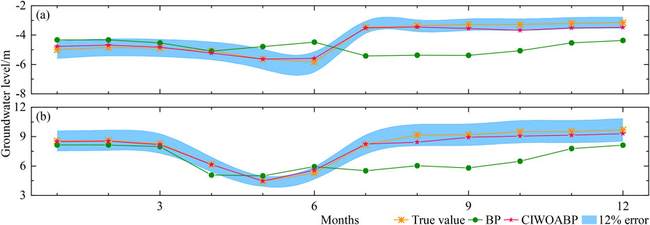
Figure 7. Comparison and analysis of different models: (A) The simulated prediction value of groundwater level in #11, and (B): The simulated prediction value of groundwater level in #12.

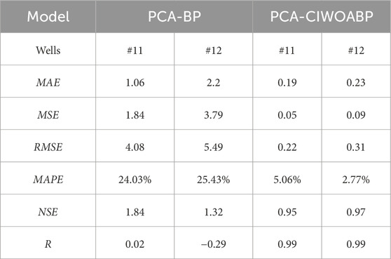
The simulation and prediction values of the BP neural network and the CIWOABP neural network exhibit significant differences. Detailed data information can be found in Table 2. The overall error of the CIWOABP neural network’s simulation prediction values is less than 12%. For monitoring wells #11 and #12, MAE is 0.19 and 0.23, MSE is 0.05 and 0.09, RMSE is 0.22 and 0.31, MAPE is 5.06% and 2.77%, NSE is 0.95 and 0.97, and R is 0.987 and 0.993, respectively. On the other hand, the BP neural network demonstrates lower prediction accuracy, with MAE values for monitoring wells #11 and #12 being 1.06 and 2.20, both exceeding 1. This indicates that the model’s generalization ability is poor, and the credibility of the simulated results is low. Based on the validation results of the two models, it can be concluded that the PCA-CIWOABP neural network established for predicting groundwater levels in the Fengnan area has high prediction accuracy, good fitting performance, and can be used to calculate and predict actual groundwater levels effectively.

Table 2

Table 2. Comparison of simulations between BP and CIWOABP.

6 Discussion

The study area of this article is located in the North China Plain, the largest “groundwater funnel” area in China, where the local government has been continuously strengthening management measures in recent years. Measures include hydrogeological investigations, development of groundwater models, zoning protection of groundwater, and pollution control and remediation of groundwater (Kløve et al., 2014; Gleeson et al., 2020). The introduction of groundwater models and development, as outlined in the introduction, primarily involve traditional hydrological models and neural network models under the drive of big data. Benefiting from local government regulations and monitoring, the availability of more hydrological information enables numerous researchers to conduct neural network research.

In this research work, it is noteworthy that although the neural network has five input and output elements, due to the limited training dataset, we introduced the PCA-CIWOA algorithm to meet the multi-input and multi-output requirements of the BP neural network. Other algorithms with similar capabilities include particle swarm optimization (Marini and Walczak, 2015), grey wolf optimization (Emary et al., 2016), and seagull optimization (Dhiman et al., 2021), each with some differences. For example, the whale optimization algorithm exhibits excellent global search capability and rapid convergence; particle swarm optimization involves information sharing and collaboration among individuals, making it suitable for continuous space optimization problems; the grey wolf algorithm combines competitive and cooperative characteristics, possessing good global search capability and convergence speed, applicable to continuous space optimization and multi-objective optimization problems. These algorithms require further comparative analysis, particularly for simulating and predicting groundwater levels in practical engineering applications.

Additionally, the interpolation methods can be used to generate images in regions with abundant water systems, and graph neural networks can be employed to achieve training and prediction results. Such as Bai and Tahmasebi (2023) represented each well as a node in a graph using a graph neural network (GNN) and utilized convolutional networks to obtain temporal features of sequences. The findings indicated that the model could achieve high simulation accuracy, even when spatial dependency relationships were completely unknown, through learning from the data. Nevertheless, the image interpolation methods are extremely important. The study employed the inverse distance interpolation method to generate groundwater level contour maps for the study area based on data from 12 monitoring wells. Xiao et al. (2016) examined seven interpolation methods, including inverse distance weighted interpolation, global polynomial interpolation, local polynomial interpolation, tension spline interpolation, ordinary Kriging interpolation, simple Kriging interpolation, and universal Kriging interpolation, to assess trends in groundwater level fluctuations in the study area. The effectiveness of these interpolation methods still needs to be further compared with actual engineering in future research work to determine their applicability.

Recently, deep learning algorithms have attracted significant attention in the field of water resources engineering. Although they are widely applicable, machine learning algorithms that rely on feature extraction still hold certain application value when the number of data samples is limited. However, when dealing with more complex multi-input and multi-output problems, the number of training samples required by deep learning algorithms far exceeds that of machine learning algorithms. Particularly in small-scale areas that urgently need remediation and have limited data samples, machine learning algorithms represented in this paper often demonstrate higher applicability than deep learning algorithms.

7 Conclusion

By reducing data dimensionality and incorporating optimization algorithms, the aim is to enhance the accuracy and stability of groundwater level simulations. The empirical research yields the following conclusions.

1. The resulting principal components (rainfall station r1, water consumption FN and QY, monitoring wells #11 and #12) still effectively represent the overall hydrological conditions in the study area, thus reducing the training complexity of the BP neural network.

2. In situations where the training samples are limited and there are multiple inputs and outputs, the BP neural network exhibits overall poor accuracy in simulating and predicting groundwater levels. The annual trend of water level changes in the simulation results may even be contrary to the actual situation.

3. The coupling of chaotic mapping and adaptive weight-based WOA significantly enhances the computational accuracy of groundwater level simulation in the BP neural network. The RMSE for monitoring wells #11 and #12 is 0.22 and 0.31, respectively, and the MAPE is 5.06% and 2.77%, respectively.

Data availability statement

The original contributions presented in the study are included in the article/supplementary material, further inquiries can be directed to the corresponding author.

Author contributions

XZ: Writing–review and editing. XG: Data curation, Writing–original draft. SL: Methodology, Writing–original draft. XS: Software, Writing–review and editing. ZX: Writing–review and editing. JZ: Writing–review and editing.

Funding

The author(s) declare that financial support was received for the research, authorship, and/or publication of this article. This work was supported by The Key Research Project in Basic Research for Colleges and Universities in Henan Province (25A570005), North China University of Water Resources and Electric Power 15th Graduate Student Innovation Project (NCWUYC-202315005), the National Natural Science Foundation of China under contract No. 41930643, “Study on carbon and nitrogen process and its effect in the Lower Yellow River”.

Conflict of interest

The authors declare that the research was conducted in the absence of any commercial or financial relationships that could be construed as a potential conflict of interest.

Publisher’s note

All claims expressed in this article are solely those of the authors and do not necessarily represent those of their affiliated organizations, or those of the publisher, the editors and the reviewers. Any product that may be evaluated in this article, or claim that may be made by its manufacturer, is not guaranteed or endorsed by the publisher.

References

Almanaseer, N., and Sankarasubramanian, A. (2012). Role of climate variability in modulating the surface water and groundwater interaction over the southeast United States. J. Hydrol. Eng. 17, 1001–1010. doi:10.1061/(ASCE)HE.1943-5584.0000536

CrossRef Full Text | Google Scholar

Bai, T., and Tahmasebi, P. (2023). Graph neural network for groundwater level forecasting. J. Hydrol. 616, 128792. doi:10.1016/j.jhydrol.2022.128792

CrossRef Full Text | Google Scholar

Bo, L., Li, Z., Liu, Y., Yue, Y., Zhang, Z., and Wang, Y. (2022). Research on multi-level scheduling of mine water reuse based on improved whale optimization algorithm. Sensors 22 (14), 5164. doi:10.3390/s22145164

PubMed Abstract | CrossRef Full Text | Google Scholar

Bowes, B. D., Sadler, J. M., Morsy, M. M., Behl, M., and Goodall, J. L. (2019). Forecasting groundwater table in a flood prone coastal city with Long short-term memory and recurrent neural networks. Water 11 (5), 1098. doi:10.3390/w11051098

CrossRef Full Text | Google Scholar

Chai, Q., Han, W., Fang, W., Ding, Z., and Wu, F. (2023). Study on coordinated allocation of conventional and unconventional water resources in typical regions of North China. Front. Earth Sci. 11. doi:10.3389/feart.2023.1198431

CrossRef Full Text | Google Scholar

Chang, F., Huang, C., Cheng, S., and Chang, L. (2017). Conservation of groundwater from over-exploitation—scientific analyses for groundwater resources management. Sci. Total Environ. 598, 828–838. doi:10.1016/j.scitotenv.2017.04.142

PubMed Abstract | CrossRef Full Text | Google Scholar

Costa, D., Zhang, H., and Levison, J. (2021). Impacts of climate change on groundwater in the Great Lakes Basin: a review. J. Gt. Lakes Res. 47 (6), 1613–1625. doi:10.1016/j.jglr.2021.10.011

CrossRef Full Text | Google Scholar

Dash, N. B., Panda, S. N., Remesan, R., and Sahoo, N. (2010). Hybrid neural modeling for groundwater level prediction. Neural comput. Appl. 19 (8), 1251–1263. doi:10.1007/s00521-010-0360-1

CrossRef Full Text | Google Scholar

Deb, S. (2024). Analyzing trends and change points in hydro-meteorological parameters and groundwater level in the Barak river basin in India. Phys. Chem. Earth 134, 103542. doi:10.1016/j.pce.2023.103542

CrossRef Full Text | Google Scholar

Demšar, U., Harris, P., Brunsdon, C., Fotheringham, A. S., and McLoone, S. (2013). Principal component analysis on spatial data: an overview. Ann. Assoc. Am. Geogr. 103 (1), 106–128. doi:10.1080/00045608.2012.689236

CrossRef Full Text | Google Scholar

Dhiman, G., Singh, K. K., Soni, M., Nagar, A., Dehghani, M., Slowik, A., et al. (2021). MOSOA: a new multi-objective seagull optimization algorithm. Expert Syst. Appl. 167, 114150. doi:10.1016/j.eswa.2020.114150

CrossRef Full Text | Google Scholar

Emary, E., Zawbaa, H. M., and Hassanien, A. E. (2016). Binary grey wolf optimization approaches for feature selection. Neurocomputing 172, 371–381. doi:10.1016/j.neucom.2015.06.083

CrossRef Full Text | Google Scholar

Gleeson, T., Cuthbert, M., Ferguson, G., and Perrone, D. (2020). Global groundwater sustainability, resources, and systems in the anthropocene. Annu. Rev. Earth Planet. Sci. 48, 431–463. doi:10.1146/annurev-earth-071719-055251

CrossRef Full Text | Google Scholar

Hosseini, Z., Gharechelou, S., Nakhaei, M., and Gharechelou, S. (2016). Optimal design of BP algorithm by ACOR model for groundwater-level forecasting: a case study on Shabestar plain, Iran. Arab. J. Geosci. 9 (6), 436. doi:10.1007/s12517-016-2454-2

CrossRef Full Text | Google Scholar

Hou, Q. Q., Pan, Y. J., Zeng, M., Wang, S., Shi, H. H., Huang, C. S., et al. (2023). Assessment of groundwater hydrochemistry, water quality, and health risk in Hainan Island, China. Sci. Rep. 13 (1), 12104. doi:10.1038/s41598-023-36621-3

PubMed Abstract | CrossRef Full Text | Google Scholar

Jolliffe, I. (2022). A 50-year personal journey through time with principal component analysis. J. Multivar. Anal. 188, 104820. doi:10.1016/j.jmva.2021.104820

CrossRef Full Text | Google Scholar

Jung, H., Ha, K., Koh, D. C., Kim, Y., and Lee, J. (2021). Statistical analysis relating variations in groundwater level to droughts on Jeju Island, Korea. J. Hydrol. Reg. Stud. 36, 100879. doi:10.1016/j.ejrh.2021.100879

CrossRef Full Text | Google Scholar

Kaur, G., and Arora, S. (2018). Chaotic whale optimization algorithm. J. Comput. Des. Eng. 5 (3), 275–284. doi:10.1016/j.jcde.2017.12.006

CrossRef Full Text | Google Scholar

Kim, G. B., Hwang, C. I., and Choi, M. R. (2021). PCA-based multivariate LSTM model for predicting natural groundwater level variations in a time-series record affected by anthropogenic factors. Environ. Earth Sci. 80 (18), 657. doi:10.1007/s12665-021-09957-0

CrossRef Full Text | Google Scholar

Kløve, B., Ala-Aho, P., Bertrand, G., Gurdak, J. J., Kupfersberger, H., Kværner, J., et al. (2014). Climate change impacts on groundwater and dependent ecosystems. J. Hydrol. 518, 250–266. doi:10.1016/j.jhydrol.2013.06.037

CrossRef Full Text | Google Scholar

Lai, V., Huang, Y. F., Koo, C. H., Ahmed, A. N., and El-Shafie, A. (2021). Optimization of reservoir operation at Klang Gate Dam utilizing a whale optimization algorithm and a Lévy flight and distribution enhancement technique. Eng. Appl. Comp. Fluid Mech. 15 (1), 1682–1702. doi:10.1080/19942060.2021.1982777

CrossRef Full Text | Google Scholar

Li, F., Feng, P., Zhang, W., and Zhang, T. (2013). An integrated groundwater management mode based on control indexes of groundwater quantity and level. Water Resour. Manag. 27 (9), 3273–3292. doi:10.1007/s11269-013-0346-8

CrossRef Full Text | Google Scholar

Li, H. H., Lu, Y. D., Zheng, C., Yang, M., and Li, S. (2019). Groundwater level prediction for the arid oasis of northwest China based on the artificial bee Colony algorithm and a back-propagation neural network with double hidden layers. Water 11 (4), 860. doi:10.3390/w11040860

CrossRef Full Text | Google Scholar

Li, M., Xu, G., Fu, Y., Zhang, T., and Du, L. (2022a). Improved whale optimization algorithm based on variable spiral position update strategy and adaptive inertia weight. J. Intell. Fuzzy Syst. 42, 1501–1517. doi:10.3233/JIFS-210842

CrossRef Full Text | Google Scholar

Li, X. Q., Lin, Q. T., Chao, K. F., and li, D. X. (2022b). A simple numerical simulation method for unsaturated stratum under the water environmental load. Comput. Geotech. 154, 105177. doi:10.1016/j.compgeo.2022.105177

CrossRef Full Text | Google Scholar

Lin, H. Y., Tseng, T. S., Wang, X., Fang, Z., Zea, A. H., Wang, L., et al. (2022). Intake patterns of specific alcoholic beverages by prostate cancer status. Cancers 14 (8), 1981. doi:10.3390/cancers14081981

PubMed Abstract | CrossRef Full Text | Google Scholar

Marini, F., and Walczak, B. (2015). Particle swarm optimization (PSO). A tutorial. Chemom. Intell. Lab. Syst. 149, 153–165. doi:10.1016/j.chemolab.2015.08.020

CrossRef Full Text | Google Scholar

Marukatat, S. (2023). Tutorial on PCA and approximate PCA and approximate kernel PCA. Artif. Intell. Rev. 56 (6), 5445–5477. doi:10.1007/s10462-022-10297-z

CrossRef Full Text | Google Scholar

Matiatos, I., Varouchakis, E. A., and Papadopoulou, M. P. (2019). Performance evaluation of multiple groundwater flow and nitrate mass transport numerical models. Environ. Model. Assess. 24 (6), 659–675. doi:10.1007/s10666-019-9653-7

CrossRef Full Text | Google Scholar

Mirjalili, S., and Lewis, A. (2016). The whale optimization algorithm. Adv. Eng. Softw. 95, 51–67. doi:10.1016/j.advengsoft.2016.01.008

CrossRef Full Text | Google Scholar

Naderianfar, M., Piri, J., and Kisi, O. (2017). Pre-processing data to predict groundwater levels using the fuzzy standardized evapotranspiration and precipitation index (SEPI). Water Resour. Manag. 31 (14), 4433–4448. doi:10.1007/s11269-017-1757-8

CrossRef Full Text | Google Scholar

Serravalle Reis Rodrigues, V. H., de Melo Barros Junior, P. R., dos Santos Marinho, E. B., and Lima de Jesus Silva, J. L. (2023). Wavelet gated multiformer for groundwater time series forecasting. Sci. Rep. 13 (1), 12726. doi:10.1038/s41598-023-39688-0

PubMed Abstract | CrossRef Full Text | Google Scholar

Singh, H., Rai, V., Kumar, N., Dadheech, P., Kotecha, K., Selvachandran, G., et al. (2023). An enhanced whale optimization algorithm for clustering. Multimed. Tools Appl. 82 (3), 4599–4618. doi:10.1007/s11042-022-13453-3

CrossRef Full Text | Google Scholar

Stigter, T. Y., Miller, J., Chen, J., and Re, V. (2023). Groundwater and climate change: threats and opportunities. Hydrogeol. J. 31 (1), 7–10. doi:10.1007/s10040-022-02554-w

CrossRef Full Text | Google Scholar

Triki, I., Trabelsi, N., Hentati, I., and Zairi, M. (2014). Groundwater levels time series sensitivity to pluviometry and air temperature: a geostatistical approach to Sfax region, Tunisia. Environ. Monit. Assess. 186 (3), 1593–1608. doi:10.1007/s10661-013--8

PubMed Abstract | CrossRef Full Text | Google Scholar

Wang, G. G., Guo, L. H., Gandomi, A. H., Hao, G. S., and Wang, H. Q. (2014). Chaotic krill herd algorithm. Inf. Sci. 274, 17–34. doi:10.1016/j.ins.2014.02.123

CrossRef Full Text | Google Scholar

Wang, W. C., Wang, B., Chau, K. W., and Xu, D. M. (2023). Monthly runoff time series interval prediction based on WOA-VMD-LSTM using non-parametric kernel density estimation. Earth Sci. Inf. 16 (3), 2373–2389. doi:10.1007/s12145-023-01038-z

CrossRef Full Text | Google Scholar

Wold, S., Esbensen, K., and Geladi, P. (1987). Principal component analysis. Chemom. Intell. Lab. Syst. 2 (1), 37–52. doi:10.1016/0169-7439(87)80084-9

CrossRef Full Text | Google Scholar

Xiao, Y., Gu, X. M., Yin, S. Y., Shao, J. L., Cui, Y. L., Zhang, Q. L., et al. (2016). Geostatistical interpolation model selection based on ArcGIS and spatio-temporal variability analysis of groundwater level in piedmont plains, northwest China. SpringerPlus 5 (1), 425. doi:10.1186/s40064-016-2073-0

PubMed Abstract | CrossRef Full Text | Google Scholar

Xu, H., Yang, X., Wang, D., Hu, Y., Shi, Y., Cheng, Z., et al. (2022). Predicting groundwater potential assessment in water-deficient islands based on convolutional neural networks. Egypt. J. Remote Sens. Space Sci. 25, 1013–1023. doi:10.1016/j.ejrs.2022.11.002

CrossRef Full Text | Google Scholar

Yan, Z., Sha, J., Liu, B., Tian, W., and Lu, J. (2018). An ameliorative whale optimization algorithm for multi-objective optimal allocation of water resources in handan, China. Water 10 (1), 87. doi:10.3390/w10010087

CrossRef Full Text | Google Scholar

Yang, X. Y., and Zhang, Z. R. (2022). A CNN-LSTM model based on a meta-learning algorithm to predict groundwater level in the middle and lower reaches of the heihe river, China. Water 14 (15), 2377. doi:10.3390/w14152377

CrossRef Full Text | Google Scholar

Zaghiyan, M. R., Eslamian, S., Gohari, A., and Ebrahimi, M. S. (2021). Temporal correction of irregular observed intervals of groundwater level series using interpolation techniques. Theor. Appl. Climatol. 145 (3), 1027–1037. doi:10.1007/s00704-021-03666-1

CrossRef Full Text | Google Scholar

Zhang, M. C. (2022). Prediction of rockburst hazard based on particle swarm algorithm and neural network. Neural comput. Appl. 34 (4), 2649–2659. doi:10.1007/s00521-021-06057-9

CrossRef Full Text | Google Scholar

Zhang, R. T., Chen, S. Z., Zhang, Z. A., and Zhu, W. C. (2022). Genetic algorithm in multimedia dynamic prediction of groundwater in open-pit mine. Comput. Intell. Neurosci. 2022, 1–6. doi:10.1155/2022/8556103

CrossRef Full Text | Google Scholar

Zhang, X. Q., Qi, Y., Li, H. Y., Wang, X., and Yin, Q. W. (2024a). Assessing the response of non-point source nitrogen pollution to land use change based on SWAT model. Ecol. Indic. 158, 111391. doi:10.1016/j.ecolind.2023.111391

CrossRef Full Text | Google Scholar

Zhang, X. Q., Ren, H., Liu, J. W., Zhang, Y. H., and Cheng, W. H. (2024b). A monthly temperature prediction based on the CEEMDAN–BO–BiLSTM coupled model. Sci. Rep. 14 (1), 808. doi:10.1038/s41598-024-51524-7

PubMed Abstract | CrossRef Full Text | Google Scholar

Zhang, X. Q., Yin, Q. W., Liu, F., Li, H. Y., and Qi, Y. (2023). Comparative study of rainfall prediction based on different decomposition methods of VMD. Sci. Rep. 13 (1), 20127. doi:10.1038/s41598-023-47416-x

PubMed Abstract | CrossRef Full Text | Google Scholar