Investigating the dynamics of water and sediment disruption due to impeller action in silt-rich reservoir zones of inland waterways in China

Introduction: This study investigates the characteristics of sediment disturbance caused by impeller rotation in reservoirs of inland rivers with high sediment content in China. A scaled experimental model, reflecting typical environmental conditions of inland water reservoirs in Northwest China, was established in Lanzhou, Gansu Province, following the principle of similarity.

Methods: The study integrates numerical simulations using Ansys Fluent software and corroborates the findings through hydraulic experiments. Computational Fluid Dynamics (CFD) and the κ–ε Realizable model were employed to simulate the solid-liquid mixing process, which was verified against the experimental model.

Results: The results indicate that increasing the impeller velocity from 2 rad/s to 8 rad/s, while submerged at a depth of 1000 mm in the flow field, enhances the rate of bottom sediment suspension. Furthermore, the rate of suspended sediment discharge from the model outlet increased with inflow velocity ranging from 0.1 m/s to 0.8 m/s. A decrease in the impeller’s submersion depth from 600 mm to 1200 mm was found to reduce the maximum disturbance radius affecting the bottom sediment.

Discussion: The reliability of the simulation was confirmed by comparing the software results with experimental data. This study provides insights into the mechanisms of sediment-laden flow disturbance in the reservoir areas of inland rivers in China and lays the groundwork for more comprehensive investigations into sediment discharge in these environments.

1 Introduction

Inland rivers across Northwest China’s inland regions, particularly in arid and semi-arid zones, are often characterized by low flow rates and high sediment loads (Chen et al., 2011; Ma et al., 2012; Yang et al., 2022). These hydrological systems typically feature scant water volumes coupled with significant sediment accumulation (Wang et al., 2023). Within such contexts, the reservoirs associated with hydroelectric stations play an integral role, as the hydroelectric generators housed within these reservoirs are pivotal in energy conversion processes (Beluco et al., 2012). Yet, in sediment-rich environments, the operation of turbine impellers induces marked disturbances within the hydrodynamic setting. Under conditions of elevated sediment, the disturbance dynamics of the two-phase water-sediment flow grow exceedingly intricate. Moreover, as disturbance duration extends, these disruptions exert a substantial influence on the impeller’s efficiency and longevity (Torotwa and Ji, 2018; Ravinath et al., 2023; Yang and Zhang, 2024).

To date, research on sediment management within sediment-heavy reservoir zones has yielded certain empirical insights. Afzalsoltani (Farid and Jafar, 2023) introduced an innovative approach to curtail reservoir siltation by strategically integrating long-term planning with intermittent flushing, thereby deriving an optimal long-term operational curve. Applied to the Dez Dam reservoir—one of Iran’s most at-risk dams—the study demonstrated that optimizing the rule curve allowed for the release of 18% of the incoming sediment over a 19-year span. Chen (Jian et al., 2021) developed a two-dimensional sediment model for a reservoir using the MIKE 21 software suite. Taking into account the specific characteristics of the PSP site’s reservoir, the model established parameters for water and sediment inflow and outflow, successfully simulating sediment dynamics within the interconnected upstream and downstream reservoir system. An analysis of 50 years’ worth of hydro-sedimentological records at the Tianchi PSP station’s downstream reservoir indicated that sediment accumulation predominantly occurs within 0.5–1.8 km upstream of the dam. After the sediment barrier was constructed over a decade ago, the average sediment depth neared 0.8 m, while sediment layers in the main river channel beyond the barrier exceeded 4.2 m. Pulendra and Kumar (2020) employed the SWAT (Soil and Water Assessment Tool) model to evaluate the potential effects of water diversion on sediment discharge. Simulating a hypothetical reservoir downstream of the India-China border, the model’s predictions highlighted the significant influence of water flow distribution on sediment transport within the area. Hussain and Shahab (2020) confirmed the sediment removal efficacy during reservoir flushing by using the HEC-RAS 5.0.6 software for numerical modeling. The study explored the model’s applicability and constraints, assessing sediment loads during non-flushing states (with a static water level at 656 m) and flushing operations, based on a 20-year sediment transport dataset from the Dasu Reservoir. Yang et al. (2015) selected the De Ri Su Bole Reservoir for their case study, investigating sediment barrier functions in sediment exclusion and control through physical models and numerical simulations. By designing a sediment barrier aligned with the reservoir’s topography and establishing a secondary reservoir zone, they reduced the sediment transit space, thereby improving the reservoir’s flushing efficiency and outperforming traditional sediment discharge designs. Blais and Bertrand (2017) demonstrated that narrowing the gap between the impeller and reservoir floor, coupled with the installation of baffles, can significantly enhance the water-sediment mixing performance, as evidenced by numerical analyses utilizing computational fluid dynamics (CFD).

The inland river systems of Northwest China’s arid regions are characterized by high sediment loads, significantly impacting hydraulic structures, particularly turbine operations in reservoir zones. Current research on the disturbance of bottom sediment due to impeller motion in these reservoirs is limited, with a focus on generating water-sediment two-phase flows for sediment expulsion. This study delves into the disturbance mechanisms of such flows induced by impeller movement in high-sediment reservoirs. Through software simulations and experimental investigations, the study elucidates the influence of impeller-induced flow on the hydrodynamics of water and sediment, as well as the resultant bottom sediment mixing. By integrating experimental data with computational fluid dynamics (CFD) simulations, the research examines the hydrodynamic behavior during sediment removal processes, endeavoring to discern the flow field and sediment displacement alterations triggered by impeller activity. The objective is to develop a theoretical framework to inform the optimization of sediment expulsion strategies for impellers in reservoir settings.

This research offers a comprehensive analysis of the water-sediment two-phase flow disturbance mechanisms during impeller rotation, providing theoretical and practical insights for the effective management and exploitation of high-sediment hydraulic resources in inland rivers. Findings enhance understanding of hydrodynamics in sediment-rich reservoirs of China’s inland waterways and bear significant implications for the sustainable operation of hydropower in the country’s western regions. The ambition of this study is to foster enduring sustainability of hydropower in Northwest China’s inland areas.

2 Application of numerical simulation of sediment-laden two-phase flow perturbation induced by impeller rotation in sediment-rich inland river reservoirs

This section discusses the implementation of three-dimensional steady-state numerical simulations using the commercial software Fluent. The focus is on the internal flow field dynamics of the cyclonic sediment discharge mechanism, utilizing the k−ε Realizable turbulence model within the Eulerian framework to examine the effects of cyclonic perturbations and flow velocity factors. The goal is to enhance the understanding of flow dynamics and sediment transport under the influence of impeller rotation in high-sediment environments.

2.1 Fundamental model and operational principle

In this research, three-dimensional, steady-state numerical simulations are performed with the commercial software Fluent to explore the internal flow field dynamics of a cyclone sediment discharge mechanism. Utilizing the k−ε Realizable turbulence model within the Eulerian context, the study examines the repercussions of cyclonic perturbations and the inherent flow velocity factors. The chosen model captures the anisotropy inherent in cyclonic turbulence, thus enhancing its aptitude for emulating the motion of rotating fluids. The pronounced pressure gradient present in cyclonic flows leads to substantial energy dissipation along the wall, necessitating the employment of the standard wall function approach to ascertain the velocity distribution proximal to the boundary. Velocity-pressure coupling resolution is facilitated by the SIMPLE implicit algorithm, grounded in the conservation equations of mass, momentum, and energy.

2.2 Three-dimensional model construction

Accounting for the research aims pertinent to sediment-rich river reservoir zones and the turbulence-inducing impeller assembly within such areas, this study leverages Solid works 2023 to craft a representative three-dimensional model. As delineated in Figure 1, the simulation experiment’s reservoir section spans dimensions of 2,516 mm × 2,448 mm × 2040 mm, boasting a length-to-diameter ratio of 13.6, an impeller diameter of 272 mm, impeller thickness of 100 mm, and quartet of blades. The rotating assembly consists of a pair of homogeneous impellers in terms of size and material, The single impeller within this assembly has a rotational domain measuring 574 mm in diameter. Table 1 provides detailed physical specifications of the impeller.

Figure 1

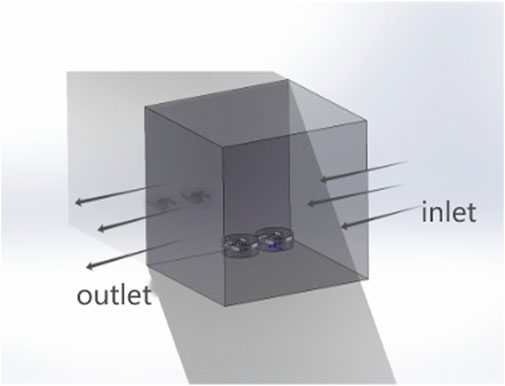
Figure 1. 3D modeling graph.

Table 1

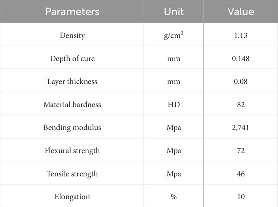
Table 1. Impeller physical parameters.

In modeling the reservoir environment, judicious selection of sand is imperative. Criteria such as sand composition, bulk density, granulometry, and viscosity must be considered in the selection process. If the native sand exhibits a coarse granulometry, then the model sand should maintain a consistent bulk density. Conversely, if the natural sand grains are fine, substituting with fine natural sand may fail to replicate sediment transport characteristics. Fine model sand is prone to flocculation, and the enhanced adhesive forces between minute particles may impede the simulation of initiation conditions. Employing larger-grain, lightweight model sand is a common workaround, which, with its reduced bulk density, more precisely mimics sediment transport dynamics on the riverbed, satisfying both the erosion and deposition similarity requisites and expediting experimental timelines. To guarantee fidelity in erosion and deposition phenomena between the model and the actual environment, the model sand’s particle size distribution must align with that of the natural sand, with the similarity criterion being near-parallelism of the respective size distribution curves.

Upon meticulous evaluation and selection, the sediment layer of 680 mm at the base and an overlying water column of 1,360 mm were established in the flow domain was established with a sediment layer of 680 mm at the base and an overlying water column of 1,360 mm. The fluid is treated as a continuous, viscous, incompressible medium under constant flow at ambient temperatures, with consideration for mass forces and channel wall roughness while neglecting surface tension effects. The stratified water and sediment diagram can be seen in Figure 2.

Figure 2

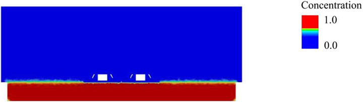
Figure 2. Water-sand stratification map. This figure illustrates the concentration distribution of water and sand within the reservoir. The x-axis represents the horizontal distance in millimeters (mm), while the y-axis represents the vertical distance in millimeters (mm). The color gradient indicates the concentration of sediment, with red representing the highest concentration (1.0) and blue indicating the lowest concentration (0.0). The figure demonstrates the stratification effect caused by sedimentation in a silt-rich environment, showcasing distinct layers of sediment concentration. The two rectangular shapes in the middle represent the impeller positions, which influence the distribution of sediments.

2.3 Mesh division and boundary conditions

Unstructured meshes are preferred for their ability to adapt to intricate boundaries, offering significant benefits in fluid dynamics and focused surface analysis. These meshes can be swiftly generated, delivering high-quality representations; additionally, the use of parametric techniques or spline function interpolation enables precise emulation of curves and surfaces, thus refining the computational domain to more accurately mirror the actual model. Therefore, this research utilized ICEM CFD software for the separate unstructured mesh subdivision of each component.

The meshing of the fluid model in ICEM CFD software begins with size adjustments in the rotating region, utilizing capture rates and setting the mesh cell size there to 5 mm. The meshing process then extends to the entire flow domain with a cell size of 20 mm. Post-mesh division, sectional views reveal an average cell quality of 0.829, a minimum orthogonal quality of 0.203, and a maximum skewness of 0.797. The mesh is relatively dense, resulting in slight deviations from actual experimental outcomes and high fidelity to real-world conditions. Examination of the mesh at the interface of the rotating area and the water body region shows excellent quality without overlaps or intersections, precluding floating-point discrepancies or errors in subsequent simulation analyses. The total mesh count stands at 7,547,413. The grid division diagram can be seen in Figure 3.

Figure 3

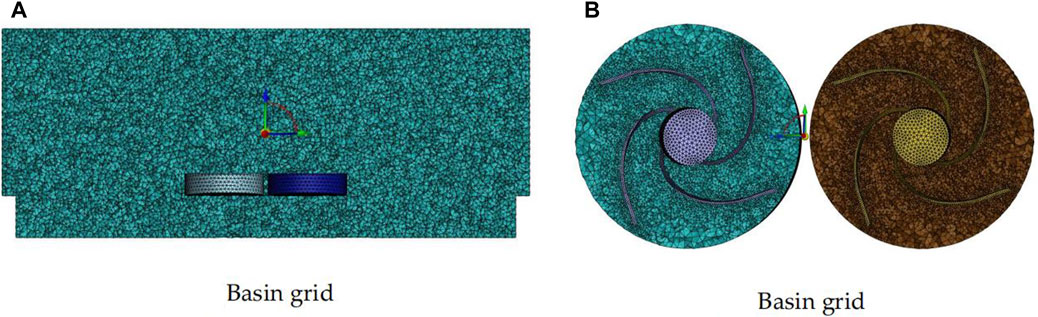
Figure 3. Area grid division. This figure presents the grid divisions used in the study.(A) Basin grid: The left panel shows the basin grid used for the simulation. The grid consists of numerous triangular elements that cover the entire basin area, ensuring detailed representation of the basin geometry and flow dynamics.(B) Impeller grid: The right panel shows the impeller grid. It consists of two views: the left sub-panel displays the impeller grid with a focus on the impeller’s blades and surrounding flow area, while the right sub-panel provides a detailed view of the grid around the impeller, highlighting the fine mesh used to capture the intricate flow patterns around the impeller blades. The grids are essential for accurate numerical simulation of water and sediment dynamics, allowing for detailed analysis of flow behavior and sediment transport influenced by the impeller action.

To ascertain the flow field characteristic variations within the cyclone sediment discharge device during operation, three-dimensional steady-state numerical computations were executed via Fluent commercial software, based on a scaled geometric model of the hydraulic water tank. The fluid domain’s water phase density is set at 1,000 kg/m³. The tank model’s upstream inlet flow employs a velocity inlet, aligned with the upstream channel’s flow direction; Solid walls are assigned a no-slip boundary condition, and near the solid wall surface, the standard wall function approach is applied for turbulent flow resolution. The tank outlet boundary uses a pressure outlet set at atmospheric pressure. The comprehensive calculation model applies standard wall functions, with the impeller wall and the rotating domain operating in a moving reference frame at 2 rad/s about the Z-axis. The overall flow domain does not use a moving reference frame; wall boundaries are no-slip conditions, the inlet is a velocity inlet with an inflow velocity of 0.8 m/s and set to liquid phase water, and the outlet is a pressure outlet with default settings; the impeller wall and rotating domain are interconnected through shared topology manipulation.

2.4 Numerical calculation method

The study utilizes the κ−ε Realizable turbulence model and transient equation to simulate hydrodynamic characteristics of water-sand two-phase flow. It adopts the SIMPLE algorithm for pressure-velocity coupling, and performs predictions on the rotational domain, impeller wall, and the distribution of water and sand phases. The mathematical models required for this study are provided in Equations 1–10.

Continuity equation:

$\frac{\partial p}{\partial t}+\frac{\partial }{\partial x_i}\left(\rho v_i\right)=0(1)$

In the equation, p represents pressure in Pascal (Pa), t represents time in seconds (s), ρ represents density in kilograms per cubic meter (kg/m³), and v represents velocity in meters per second (m/s).

Time-averaged liquid phase continuity equation:

$\frac{\partial {\varphi }_f}{\partial t}+\frac{\partial }{\partial x_i}\left({\varphi }_f{V}_{fi}-\frac{v_t}{{\sigma }_{\varphi f}}\frac{\partial {\varphi }_f}{\partial x_i}\right)=0(2)$

In the equation, ϕ_f represents a physical quantity of the liquid (such as concentration or mass fraction) in kilograms per cubic meter (kg/m³), t represents time in seconds (s), v represents the velocity vector of the liquid in meters per second (m/s), V_fi represents the volume of the liquid in cubic meters (m³), and σ represents the normal stress in Pascal (Pa).

Time-averaged solid phase continuity equation:

$\frac{\partial {\varphi }_s}{\partial t}+\frac{\partial }{\partial x_i}\left({\varphi }_s{V}_{si}-\frac{v_t}{{\sigma }_{\varphi s}}\frac{\partial {\varphi }_s}{\partial x_i}\right)=0(3)$

In the equation, ϕ_s represents a physical quantity of the solid (such as concentration or mass fraction) in kilograms per cubic meter (kg/m³), t represents time in seconds (s), v represents the velocity vector of the solid in meters per second (m/s), and V_si represents the volume of the solid in cubic meters (m³).

Time-averaged liquid phase momentum equation:

$\begin{array}{l}\frac{\partial }{\partial t}\left({\varphi }_f{V}_{fi}\right)+\frac{\partial }{\partial x_j}\left({\varphi }_f{V}_{fi}{V}_{fj}\right)\\ =\frac{\partial }{\partial x_j}\left[\frac{v_t}{{\sigma }_{\varphi f}}\left(V_{fi}\frac{\partial {\varphi }_f}{\partial x_j}+V_{fj}\frac{\partial {\varphi }_f}{\partial x_i}\right)-{\varphi }_f\overline{v_{fi}{v}_{fj}}\right]\\ -\frac{1}{{\rho }_f}\left({\varphi }_f\frac{\partial p}{\partial x_i}+{\varphi }_f\frac{\partial p^{\prime }}{\partial x_i}\right)+v_f\frac{\partial }{\partial x_j}\left[{\varphi }_f\left(\frac{\partial V_{fi}}{\partial x_j}+\frac{\partial V_{fj}}{\partial x_i}\right)\right]\\ -\frac{B}{{\rho }_f}\left[{\varphi }_f{\varphi }_s\left(V_{fi}-V_{si}\right)+\left({\varphi }_s-{\varphi }_f\right)\left(\frac{v_t}{{\sigma }_{\varphi s}}-\frac{v_t}{{\sigma }_{\varphi f}}\right)\frac{\partial {\varphi }_f}{\partial x_i}\right]+{\varphi }_f{g}_i\end{array}(4)$

In the equation, ρ represents density in kilograms per cubic meter (kg/m³), t represents time in seconds (s), v_f represents the velocity vector of the liquid in meters per second (m/s), p represents pressure in Pascal (Pa), and g represents the acceleration due to gravity in meters per second squared (m/s²) (taking g = −9.81 m/s²); Time-averaged solid phase momentum equation:

$\begin{array}{l}\frac{\partial }{\partial t}\left({\varphi }_s{V}_{si}\right)+\frac{\partial }{\partial x_j}\left({\varphi }_s{V}_{si}{V}_{sj}\right)\\ =\frac{\partial }{\partial x_j}\left[\frac{v_t}{{\sigma }_{\varphi s}}\left(V_{si}\frac{\partial {\varphi }_s}{\partial x_j}+V_{sj}\frac{\partial {\varphi }_s}{\partial x_i}\right)-{\varphi }_s\overline{v_{si}{v}_{sj}}\right]\\ -\frac{1}{{\rho }_s}\left({\varphi }_s\frac{\partial p}{\partial x_i}+{\varphi }_f\frac{\partial p^{\prime }}{\partial x_i}\right)+v_s\frac{\partial }{\partial x_j}\left[{\varphi }_s\left(\frac{\partial V_{si}}{\partial x_j}+\frac{\partial V_{sj}}{\partial x_i}\right)\right]\\ -\frac{B}{{\rho }_s}\left[{\varphi }_f{\varphi }_s\left(V_{si}-V_{fi}\right)+\left({\varphi }_f-{\varphi }_s\right)\left(\frac{v_t}{{\sigma }_{\varphi s}}-\frac{v_t}{{\sigma }_{\varphi f}}\right)\frac{\partial {\varphi }_s}{\partial x_i}\right]+{\varphi }_s{g}_i\end{array}(5)$

In the equation, ρ represents density in kilograms per cubic meter (kg/m³), t represents time in seconds (s), v_s represents the microscopic velocity vector of the solid particles in meters per second (m/s), σ represents the normal stress in Pascal (Pa), and g represents the acceleration due to gravity in meters per second squared (m/s²) (taking g = −9.81 m/s²).

The turbulent kinetic energy equation (κ equation) for two-phase flow of solid and liquid is

$\begin{array}{l}\frac{\partial }{\partial t}\left({\varphi }_{f}k\right)+\frac{\partial }{\partial x_j}\left({\varphi }_f{V}_{fj}k\right)=\frac{\partial }{{\partial }_{\varphi f}}\left(\frac{v_t}{{\sigma }_{\varphi f}}{\varphi }_f\frac{\partial k}{\partial x_i}\right)-{\varphi }_f\epsilon \\ +P_r+V_{Df}+A_{Ds}\end{array}(6)$

In the equation, ϕ_f represents a physical quantity of the liquid (such as concentration or mass fraction) in kilograms per cubic meter (kg/m³),t represents time in seconds (s), k represents turbulent kinetic energy in square meters per second squared (m²/s²), v represents velocity vector in meters per second (m/s), and ε represents turbulent dissipation rate in cubic meters per second cubed (m²/s³).

The turbulent dissipation rate equation (ε equation) for two-phase flow of solid and liquid is a crucial component in understanding the dynamics of such systems.

$\begin{array}{l}\frac{\partial }{\partial t}\left({\varphi }_f\epsilon \right)+\frac{\partial }{\partial x_j}\left({\varphi }_f{V}_{fj}\epsilon \right)\\ =\frac{\partial }{\partial x_j}\left[\left(v_f+\frac{v_t}{{\sigma }_{\epsilon }}\right){\varphi }_f\frac{\partial \epsilon }{\partial x_j}\right]+\left[C_{\epsilon 1}{P}_r-{\varphi }_f\left(C_{\epsilon 2}\epsilon +C_{\epsilon 3}{A}_{Ds}\right)\right]\frac{\epsilon }{k}\end{array}(7)$

In the equation,ε represents turbulent dissipation rate in cubic meters per second cubed (m²/s³), v represents velocity vector in meters per second (m/s), and μ represents dynamic viscosity of the fluid in kilograms per meter per second (kg/(m·s).

Where:

$\begin{array}{l}\overline{{\varphi }_f\frac{\partial p^{\prime }}{\partial x_i}}=-{\rho }_f\frac{\partial }{\partial x_i}\left[\left(C_1{k}^{1/2}+C_2\frac{k^{3/2}}{\epsilon }\frac{\partial V_{fi}}{\partial x_k}\right)\frac{v_t}{{\sigma }_{\varphi f}}\frac{\partial {\varphi }_f}{\partial x_k}\right]\\ +{\rho }_f\frac{\epsilon }{k}\left[C_3\overline{{\varphi }_f{\upsilon }_{fi}}+C_4\left(\frac{1}{k}\overline{{\upsilon }_{fj}{\upsilon }_{fk}}+\frac{2}{3}{\delta }_{ik}\frac{v_t}{{\sigma }_{\varphi f}}\frac{\partial {\varphi }_f}{\partial x_k}\right)\right]\\ -{\rho }_f\left(C_5\frac{\partial V_{fi}}{\partial x_k}+C_6\frac{\partial V_{fk}}{\partial x_i}\right)\frac{v_t}{{\sigma }_{\varphi f}}\frac{\partial {\varphi }_f}{\partial x_i}\end{array}(8)$

$\begin{array}{l}{p}_r=\frac{\partial }{\partial x_j}\left(\frac{v_t}{{\sigma }_{\varphi f}}{V}_{fi}{V}_{fj}\frac{\partial {\varphi }_f}{\partial x_i}-V_{fi}\overline{{\phi }_f{\upsilon }_{fi}{\upsilon }_{fj}}-V_{fj}\overline{{\phi }_f{\upsilon }_{fi}^2}\right)\\ -\frac{\partial }{\partial x_j}\left({\varphi }_f{V}_{fi}\right)\overline{{\upsilon }_{fi}{\upsilon }_{fj}}+\frac{1}{{\rho }_f}\frac{v_t}{{\sigma }_{\varphi f}}\frac{\partial {\varphi }_f}{\partial x_j}\frac{\partial p}{\partial x_j}\\ -C_k\frac{v_t}{{\sigma }_{\varphi f}}\frac{k}{\epsilon }\left(V_{fi}\frac{\partial {\varphi }_f}{\partial x_j}+V_{fj}\frac{\partial {\varphi }_f}{\partial x_i}\right)\end{array}(9)$

$V_{Df}=v_f\left\{\begin{array}{l}{\varphi }_f\frac{{\partial }^{2}k}{\partial x_j^2}+\frac{\partial {\varphi }_f}{\partial x_j}\left(\frac{\partial k}{\partial x_j}+\frac{\partial \overline{{\upsilon }_{fi}{\upsilon }_{fj}}}{\partial x_i}+v_t\frac{{\partial }^2{V}_{fi}}{\partial x_j^2}\right)\\ -\frac{\partial }{\partial x_j}\left[\frac{v_t}{{\sigma }_{\varphi f}}\frac{\partial {\varphi }_f}{\partial x_i}\left(\frac{\partial V_{fi}}{\partial x_j}+\frac{\partial V_{fj}}{\partial x_i}\right)\right]\end{array}\right\}(10)$

In the above equation, the subscripts i, j, and k represent different components of the tensor. t represents time, V_i represents the time-averaged velocity component, v_i represents the fluctuating velocity component, x_i represents the component of the coordinate, P represents the time-averaged pressure, p' represents the fluctuating pressure, φ represents the time-averaged volume fraction (concentration), ϕ represents the fluctuating volume fraction, g_i represents the component of the gravitational acceleration in the i direction, ρ represents the material density, and μ represents the dynamic viscosity of the material.

2.5 Grid independence verification

The grid count influences both calculation precision and the time required for computation. Fewer grids can accelerate the solution process and reduce computational duration but may compromise accuracy. In contrast, more grids enhance precision at the expense of increased computational resources and time. Conducting grid independence verification is thus essential to confirm the accuracy of numerical simulation results. To maintain computational accuracy, each component’s grid quality is kept above 0.4. Upon grid assembly completion, grid independence verification was conducted at total grid counts of 498,000, 573,100, 754,700, and 935,700.

The verification results show that when the total number of grids is 754,700, the error with respect to the adjacent control group is controlled within 2%, which means that it is possible to obtain relatively precise results while effectively saving computational time (See Figure 4).

Figure 4

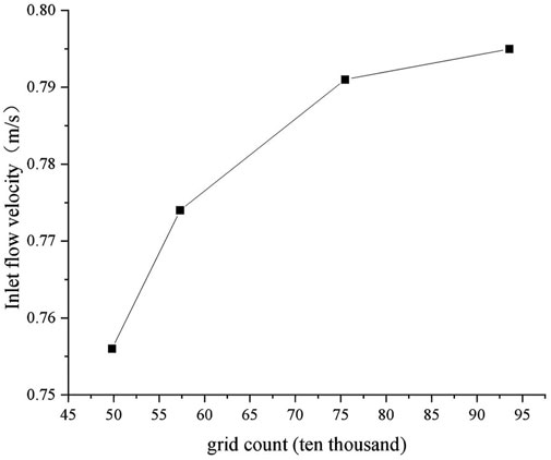
Figure 4. Mesh independence verification.

The verification results demonstrate that with a grid total of 754,700, the error relative to the adjacent control group is maintained within 2%. This suggests that highly accurate outcomes are achievable while also ensuring significant savings in computational effort. The grid count and node distribution across each computational domain within the model structure are detailed in Table 2.

Table 2

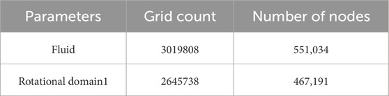
Table 2. Total number of cells and grid nodes within each computational domain.

3 Development and analysis of a comprehensive system mathematical model for submergence depth, inlet flow velocity, and impeller rotation speed

3.1 Analysis of inundation depth

Numerical simulations were conducted at an impeller rotation speed of 6 rad/s and an inlet flow velocity of 0.8 m/s, The impeller submersion depths varied at 1,200 mm, 1,000 mm, 800 mm, and 600 mm, respectively. The results, depicting the distribution of impeller pressure, particle concentration, and velocity vectors, are shown in the provided figures.

With increasing submersion depth, the hydrostatic pressure exerted on the impeller rises due to the direct proportionality of water pressure to depth. This means that pressure under static conditions equates to the density of water multiplied by gravitational acceleration and depth. Additionally, the rotational motion of the impeller leads to a rise in fluid velocity and a corresponding decrease in static pressure, creating a low-pressure zone that sustains the disturbance effect of the impeller’s rotation. Analysis of the particle concentration distribution suggests that the low-pressure conditions in the rotation zone cause sediment particles to accumulate, potentially due to vortex formation and particle inertia. These vortices, generated by the rotating impeller, influence the trajectory of particles, due to their inertia hindering rapid movement with the fluid (See Figure 5).

Figure 5

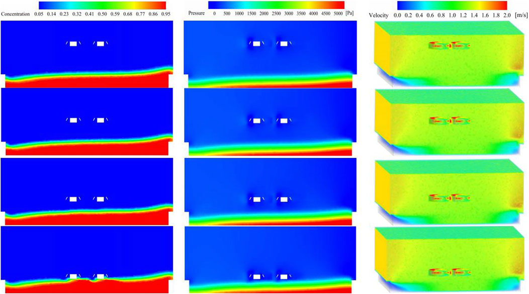
Figure 5. Pressure distribution, concentration distribution, and vector distribution at submergence depths of 1,200, 1,000, 800, and 600 mm. This figure illustrates the simulation results at various impeller submergence depths, showing the distribution of concentration, pressure, and velocity. Horizontal axis: Represents different impeller submergence depths (1,200 mm, 1,000 mm, 800 mm, and 600 mm). Vertical axis:Top row: Concentration distribution (dimensionless). Middle row: Pressure distribution (Pa). Bottom row: Velocity distribution (m/s). The concentration distribution images show the variation of sediment concentration with red indicating higher concentration and blue indicating lower concentration. The pressure distribution images highlight the pressure variations in the flow field with corresponding color scales. The velocity distribution images depict the flow velocity around the impellers, indicating flow patterns and intensities.

The velocity vector distribution analysis indicates that fluid flow complexity increases in proximity to the rotating impeller. The flow velocity near the impeller accelerates markedly, suggesting that the disturbance from the high-speed rotation is effective in converting bottom sediment to suspended sediment, which is then expelled with the water flow. The numerical simulation analysis reveals that impeller pressure intensifies with increasing submersion depth, and the low-pressure zone created by rotation impacts particle movement and deposition. Nevertheless, the disturbance from the high-speed rotation of the impeller more effectively transforms bottom sediment into suspended sediment, thus enhancing the efficiency of sediment particle discharge.

3.2 Inlet flow velocity analysis

Simulations were performed at an impeller rotation speed of 6 rad/s and a submersion depth of 1,000 mm, with inlet velocities of 0.1 m/s, 0.3 m/s, 0.5 m/s, and 0.8 m/s. The outcomes, reflecting changes in impeller pressure, particle concentration, and velocity vector distribution, are displayed in the figures (See Figure 6).

Figure 6

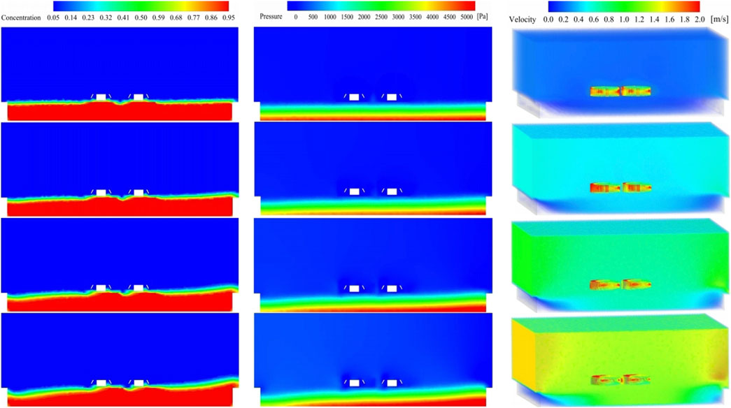
Figure 6. Pressure distribution, concentration distribution, and vector distribution at inlet flow velocities of 0.1, 0.3, 0.5, and 0.8 m/s. This figure illustrates the simulation results at various inlet flow velocities, showing the distribution of concentration, pressure, and velocity. Horizontal axis: Represents different inlet flow velocities (0.1 m/s, 0.3 m/s, 0.5 m/s, and 0.8 m/s). Vertical axis:Top row: Concentration distribution (dimensionless). Middle row: Pressure distribution (Pa). Bottom row: Velocity distribution (m/s). The concentration distribution images display the variation of sediment concentration, with red indicating higher concentration and blue indicating lower concentration. The pressure distribution images show the pressure variations in the flow field with corresponding color scales. The velocity distribution images depict the flow velocity around the impellers, highlighting flow patterns and intensities.

Trends in the distribution of impeller pressure, particle concentration, and velocity vectors correlate with inlet velocity variations. At 0.1 m/s inlet velocity, the impeller experiences lower pressure. As the inlet velocity escalates, the impeller pressure distribution increases, peaking at 0.5 m/s. Beyond this point, a further increase to 0.8 m/s reduces the pressure, albeit remaining elevated. This indicates that an optimal inlet flow velocity can enhance the impeller’s operational efficiency and promote the conversion of bottom sediment to suspended material.

At an inlet velocity of 0.1 m/s, particle concentration distribution is observed to be lower. With increasing inlet velocities, there is a corresponding gradual rise in particle concentration distribution. However, at an elevated inlet velocity of 0.8 m/s, although there is a decrease in the particle concentration distribution, it remains substantially high. This phenomenon indicates that at an inlet velocity of 0.8 m/s, the rate of bottom sediment erosion and subsequent removal by the water significantly increases, suggesting a directly proportional relationship between inlet velocity and sediment discharge rate. At the initial velocity of 0.1 m/s, velocity vector distribution is narrowed with reduced flow velocities near the impeller. As the inlet velocity increases, also increases the extent of velocity vector distribution. Upon further increase to 0.8 m/s, velocity vectors peak, exhibiting the highest flow velocities surrounding the impeller. This denotes that elevated inlet velocities enhance the distribution of velocity vectors around the impeller, which in turn augments the agitation of bottom sediment.

In scenarios where the impeller operates at a rotation speed of 8 rad/s with a submersion depth of 1,000 mm, inlet flow velocity significantly impacts impeller pressure, particle concentration, and velocity vector distribution. An optimal inlet flow velocity enhances the impeller’s operational efficiency, increases the disturbance of bottom sediment, promotes the conversion of sediment to suspended material, and facilitates sediment discharge.

3.3 Impeller rotation speed analysis

Under specific conditions, including an inlet flow velocity of 0.8 m/s and a submersion depth of 1,000 mm, numerical simulations were carried out at impeller rotation speeds of 2, 4, 6, and 8 rad/s. The simulations yielded data for the impeller pressure, particle concentration, and velocity vector distributions, which are illustrated in the figures (See Figure 7).

Figure 7

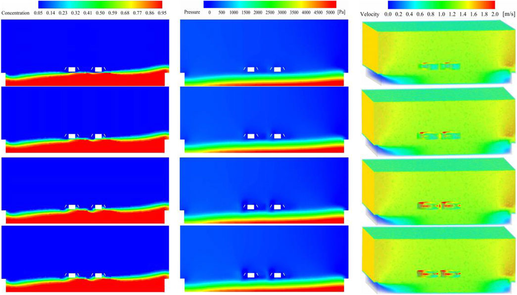
Figure 7. Pressure distribution, concentration distribution, and vector distribution at impeller rotational speeds of 2, 4, 6, and 8 rad/s. This figure illustrates the simulation results at various impeller rotational speeds, showing the distribution of concentration, pressure, and velocity. Horizontal axis: Represents different impeller rotational speeds (2 rad/s, 4 rad/s, 6 rad/s, and 8 rad/s). Vertical axis:Top row: Concentration distribution (dimensionless). Middle row: Pressure distribution (Pa). Bottom row: Velocity distribution (m/s). The concentration distribution images display the variation of sediment concentration, with red indicating higher concentration and blue indicating lower concentration. The pressure distribution images show the pressure variations in the flow field with corresponding color scales. The velocity distribution images depict the flow velocity around the impellers, highlighting flow patterns and intensities.

At 2 rad/s, the impeller experiences a relatively modest pressure distribution. With incremental increases in rotation speed, there is a corresponding rise in pressure distribution, which is particularly notable at 6 rad/s, where the pressure distribution reaches a zenith. Advancing the rotation speed to 8 rad/s results in a diminished pressure distribution trend, yet it maintains a high level. This is attributable to the formation of a low-pressure zone adjacent to the impeller at high rotational speeds, which reduces the pressure distribution at 8 rad/s. Within a certain threshold, an increase in impeller rotation speed amplifies the pressure exerted on the impeller, thereby enhancing the disturbance efficiency of bottom sediment.

A gradual increase in impeller rotation speed significantly affects particle concentration distribution. At 2 rad/s, the particle concentration distribution is relatively minimal. However, as the impeller rotation speed rises, so does the particle concentration distribution, reaching a pinnacle at 6 rad/s. An increase to 8 rad/s results in a downward trend in the particle concentration distribution, though it remains pronounced. This pattern emerges because the high-speed rotation of the impeller generates a negative pressure area and swift vortices near the impeller, which entrap sediment particles within the rotational zone and hinder their discharge. Consequently, an apt impeller rotation speed can expedite the stirring of bottom sediment, thereby optimizing sediment discharge efficiency. The distribution of velocity vectors at different rotation speeds shows that at 2 rad/s, the distribution near the impeller is significantly low. As the impeller rotation speed increases, the velocity distribution near the impeller rises, reaching its peak at 8 rad/s. This signifies that a higher impeller rotation speed refines the velocity vector distribution adjacent to the impeller, elevates fluid velocity proximate to the impeller, and promotes the suspension and segregation of bottom sediment, culminating in an improved sediment discharge efficacy.

Under conditions where the inlet flow velocity is set at 0.8 m/s and the submersion depth at 1,000 mm, the rotational speed of the impeller markedly influences its pressure generation, particle concentration, and the distribution of velocity vectors. Within a specific range, an increase in the rotational speed of the impeller enhances sediment discharge efficiency. However, excessively high speeds lead to reductions in both pressure and particle concentration distributions, attributable to the formation of negative pressure zones and high-speed vortices within the impeller’s rotational domain. Thus, a moderate increase in the impeller’s rotational speed is advisable to augment the agitation of bottom sediments and boost efficiency in sediment discharge.

4 Experimental verification of physical model construction and reliability analysis

4.1 Physical model construction

To investigate the disturbance effects on water and sediment by impeller rotation in sediment-rich reservoir regions of inland rivers and to validate these observations against numerical simulations, a physical model was established in Lanzhou City, Gansu Province, China, as depicted in Figure 8. The apparatus comprises a water supply system, a hydraulic system, and a cyclone sediment discharge unit, among other components. A flow regulation device at the model’s inlet enables precise control of the inlet flow velocity, ensuring experimental accuracy. In addition, the cyclone sediment discharge unit requires synchronized operational speeds, with exact rotational speed control, to align experimental outcomes more closely with the data constraints, thereby enhancing the results’ credibility.

The water supply system is designed as a closed loop to conserve water resources. The water utilized in the experiments is recycled, necessitating the installation of a tailwater treatment system at the experiment’s conclusion to handle the effluent water-sediment mixture. The treated water is then recirculated to the experimental inlet.

The physical impeller, shown in Figure 8, was constructed from materials detailed in Table 1 of Chapter 1. The impeller components are connected to the cyclone sediment discharge unit via a rotating shaft, ensuring uniform rotational speeds and maximizing the impeller assembly’s disturbance efficacy.

In the physical model experiment, the dimensions of the reservoir area’s flow domain are 185 mm × 180 mm × 150 mm (See Figure 8).

Figure 8

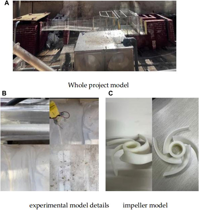
Figure 8. Experimental model. (A) Whole project model. (B) experimental model details. (C) impeller model.

4.2 Reliability verification

To ascertain the numerical simulations’ precision, they were juxtaposed with physical experimental data. Points of detection were set at varying submersion depths—1200 mm, 1,000 mm, 800 mm, and 600 mm—to gauge and compare environmental pressure around the impeller, particle concentration distribution, and sand discharge velocity. The corresponding results are illustrated in the figures. Data from these numerous points closely matched the experimental values, confirming the high reliability of the simulations at a submersion depth of 1,000 mm and laying a robust groundwork for further experimental inquiry.

Statistical analysis was employed to evaluate the correlation between simulation and experimental data, using metrics such as Pearson’s correlation coefficient and root mean square error (RMSE) to quantify the degree of alignment and error margins.

Additionally, inlet flow velocity was examined as an additional variable. Detection points at varying velocities—0.1 m/s, 0.3 m/s, 0.5 m/s, and 0.8 m/s—were set up for comparing measurements of environmental pressure, particle concentration, and sand discharge velocity. The results, The results shown in the figures, closely correlate with experimental values, especially at an inlet flow velocity of 0.8 m/s, which is considered optimal for high reliability. This velocity serves as a boundary condition for future experiments.

Chapter 2 presented experimental findings regarding the impact of impeller rotation speed on sand discharge efficiency, pinpointing the most significant effect at 6 rad/s. Consequently, this speed was adopted as the benchmark for experimental reliability verification. The impeller rotation speed of 6 rad/s served as a constraint for numerical simulation reliability checks, with the verification outcomes presented in Figure 9.

Figure 9

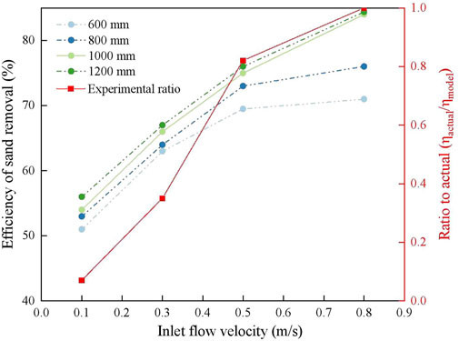
Figure 9. Reliability verification.

Upon verification of reliability through both physical and computational models, we have ascertained that under specific conditions—namely, impeller submersion depths of 1,200 mm and 1,000 mm, inlet flow velocities of 0.5 m/s and 0.8 m/s, and an impeller rotation speed of 6 rad/s—the outcomes align closely with experimental data. The consistency and reliability of these results were further confirmed through statistical tests, ensuring that the findings are robust and statistically significant. These findings are pivotal in determining the most efficacious settings for sand discharge, providing a foundation for further research on sediment management in inland river reservoirs with high siltation.

5 Analysis and discussion

5.1 Insights into impeller submersion depth in reservoir areas

The submersion depth of impellers is a paramount factor influencing the efficiency of sand removal systems. In designing such depths for inland river reservoirs, one must consider the implications on sand removal efficacy. Simulations indicate a direct correlation between impeller submersion depth and the pressure exerted on it. Excessive depths lead to augmented environmental pressure, potentially resulting in impeller damage, increased energy consumption, and heightened operational resistance.

Additionally, analyses of particle density distribution at greater submersion depths demonstrate that sediment tends to accumulate within the impeller’s rotational zone. This is a consequence of the pressure differential introduced by the impeller. The pressure differential, amplified by elevated depths, traps this pressure differential, which traps sediment in the rotational area, hindering its expulsion.

Therefore, the selection of an optimal submersion depth is crucial for augmenting sand discharge efficiency, balancing the mitigation of high-pressure risks and enhancing sediment removal, thus improving the overall performance of the sand removal system (See Figure 10). In Figure 10A represents the static pressure distribution diagram; Figure 10B represents the volume fraction diagram; Figure 10C represents the velocity magnitude diagram.

Figure 10

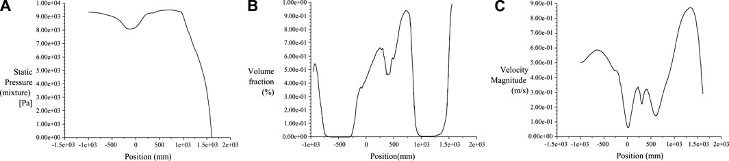
Figure 10. Discussion on the pressure distribution, concentration distribution, and vector distribution with varying submergence depths. (A) represents the static pressure distribution diagram; (B) represents the volume fraction diagram; (C) represents the velocity magnitude diagram.

5.2 Evaluating impeller rotation and inlet flow velocity in reservoir areas

Inlet flow velocity is a significant determinant of sand discharge efficiency. Naturally, water flow mobilizes bottom sediment, a process that intensifies with increasing flow velocity. However, this natural process is slow and can lead to secondary sediment deposition. By adjusting the inlet flow velocity in tandem with impeller agitation, one can bolster the efficiency of sand discharge.

Nevertheless, when employing an impeller assembly, it is not merely a matter of increasing the inlet flow velocity for sediment scouring. The optimal combination of these factors must be assessed to maximize sediment removal. Empirical evidence suggests that a velocity of 0.5 m/s is optimal for sand removal. Elevating the velocity to 0.8 m/s increases the pressure on the impeller, raising energy demands and accelerating wear, which is detrimental to sustained operation. While a higher velocity may facilitate sediment discharge, impeller longevity and material costs must also be factored in.

Thus, a moderate increase in inlet flow velocity, when used with an impeller assembly, can indeed improve the expulsion of suspended sediment. An optimal increase in inlet flow velocity can boost sand removal efficiency; however, it is essential to strike a balance between effective sediment removal and the durability and cost-efficiency of the impeller assembly (See Figure 11). In Figure 11A represents the static pressure distribution diagram; Figure 11B represents the volume fraction diagram; Figure 11C represents the velocity magnitude diagram.

Figure 11

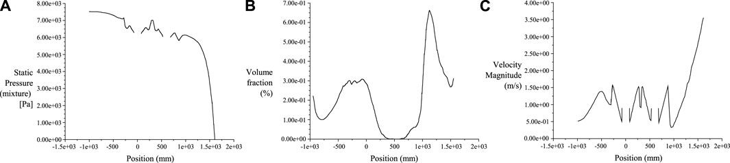
Figure 11. Discussion of the pressure distribution, concentration distribution, and vector distribution with varying inlet flow velocities. (A) represents the static pressure distribution diagram; (B) represents the volume fraction diagram; (C) represents the velocity magnitude diagram.

5.3 Discussion on impeller rotation speed in reservoir areas

The rotation speed of the impeller is a pivotal parameter for enhancing sand removal efficiency. An increase in the impeller’s rotation speed augments the agitation of bottom sediments, facilitating their transition into suspended sediment particles and boosting the efficiency of this process. The relationship between efficiency and impeller rotation speed is directly proportional. Nevertheless, numerical simulation experiments have demonstrated that, while escalating the impeller rotation speed from 2 rad/s to 6 rad/s optimizes sand removal efficiency, a further increase to 8 rad/s imposes additional pressure on the impeller. The negative pressure region generated by the rotating impeller experiences a decrease in pressure, leading to a substantial pressure gradient relative to the surrounding environment. This exacerbates stress on the impeller blades and accelerates wear, curtailing the impeller’s service life and adversely impacting long-term functionality (See Figure 12). In Figure 12A represents the static pressure distribution diagram; Figure 12B represents the volume fraction diagram; Figure 12C represents the velocity magnitude diagram.

Figure 12

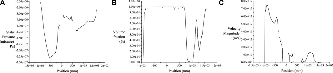
Figure 12. Discussion of the pressure distribution, concentration distribution, and vector distribution with varying inlet flow velocities. (A) represents the static pressure distribution diagram; (B) represents the volume fraction diagram; (C) represents the velocity magnitude diagram.

High impeller rotation speeds induce a significant pressure disparity between the impeller environment and the adjacent water body, impeding the ejection of sediment particles entrapped by the negative pressure and high-speed vortex. Therefore, it is challenging to expel these particles even with increased inlet flow velocity. An appropriate increment in the impeller rotation speed can indeed heighten sand removal efficiency. Within a specific range, this increment improves bottom sediment agitation, aiding their conversion into suspended sediment particles and thus, enhancing efficiency. However, it also adds to the impeller’s pressure burden. Consequently, when enhancing the impeller rotation speed, it is essential to consider its impact on the pressure exerted on the impeller. Adjusting the speed to remain within the impeller’s endurance threshold is crucial for sustainably improving sand removal efficiency.

6 Conclusion

(1) Numerical simulations of the water tank show that the disturbance efficiency of the swirling flow, generated by the cyclone sand removal device, depends on both the submersion depth and the rotation speed. With a parallel and aligned impeller assembly, the flow field disturbance increases with impeller rotation speed. However, beyond 6 rad/s, the rate of increase in disturbance efficiency diminishes, signifying that impeller rotation speed is instrumental in influencing disturbance efficiency within the region.

(2) Model experiments with the cyclone sand removal device, conducted at varying incoming flow velocities, have indicated that under conditions of scouring and silting, the particle distribution changes in a manner that mirrors the incoming flow velocity; as the latter increases, so does the sand removal efficiency. The relationship between high sand removal efficiency and incoming flow velocity is pronounced, particularly at elevated velocities.

(3) The outcomes of model experiments, considering varied changes in the cyclone sand removal device, provide a theoretical basis for future research exploring the effects of the number of impellers, their rotation angles, and the positioning of the impeller assembly on sand removal efficacy in reservoir areas.

Data availability statement

The original contributions presented in the study are included in the article/supplementary material, further inquiries can be directed to the corresponding author.

Author contributions

HW: Methodology, Writing–original draft, Writing–review and editing. YW: Conceptualization, Writing–review and editing. KL: Validation, Writing–review and editing. TL: Validation, Writing–review and editing. JL: Formal Analysis, Writing–review and editing. YZ: Resources, Writing–review and editing. TM: Resources, Writing–review and editing. MT: Writing–original draft. ZW: Funding acquisition, Writing–review and editing. XZ: Funding acquisition, Writing–review and editing.

Funding

The author(s) declare that financial support was received for the research, authorship, and/or publication of this article. National Natural Science Foundation of China, Regional Fund: Study on the Mechanism of Heavy Metal Migration and Transformation in Alpine Inland Rivers Due to Cascading Dam Construction (52169015); China’s National Key Research and Development Program: Targeted Depolymerization and Enhanced Pretreatment Technology for Diversified Biomass Alcohol Feedstocks (2022YFB4201901-1); Gansu Province Water Resources Scientific Research and Technology Promotion Project of China, 2023 (23GSLK032).

Acknowledgments

We also are grateful to the editor and reviewers for their thoughtful comments on this manuscript.

Conflict of interest

The authors declare that the research was conducted in the absence of any commercial or financial relationships that could be construed as a potential conflict of interest.

Publisher’s note

All claims expressed in this article are solely those of the authors and do not necessarily represent those of their affiliated organizations, or those of the publisher, the editors and the reviewers. Any product that may be evaluated in this article, or claim that may be made by its manufacturer, is not guaranteed or endorsed by the publisher.

References

Beluco, A., Souza, P. K. D., and Krenzinger, A. (2012). A method to evaluate the effect of complementarity in time between hydro and solar energy on the performance of hybrid hydro PV generating plants. Renew. Energy 45, 24–30. doi:10.1016/j.renene.2012.01.096

CrossRef Full Text | Google Scholar

Blais, B., and Bertrand, F. (2017). CFD-DEM investigation of viscous solid-liquid mixing: impact of particle properties and mixer characteristics. Chem. Eng. Res. Des. 118, 270–285. doi:10.1016/j.cherd.2016.12.018

CrossRef Full Text | Google Scholar

Chen, Y., Li, B., Fan, Y., Sun, C., Fang, G., Zong, Q., et al. (2011). Hydrological processes and water cycle of inland river basins in the arid regions of Northwest China: challenges of low flow rates and high sediment loads. J. Hydrology 41 (Null) (SpringerLink).

Google Scholar

Farid, A., and Jafar, Y. (2023). Development of a model for sediment evacuation from reservoirs. Environ. Process. 10 (3), 46. doi:10.1007/s40710-023-00660-9

CrossRef Full Text | Google Scholar

Hussain, K., and Shahab, M. (2020). Sustainable sediment management in a reservoir through flushing using HEC-RAS model: case study of Thakot Hydropower Project (D-3) on the Indus river. Water Supply 20 (2), 448–458. doi:10.2166/ws.2019.174

CrossRef Full Text | Google Scholar

Jian, C., Qin, L., Xin, L., Wang, H., Zhang, Y., Liu, X., et al. (2021). Research on the application of 2-D sediment mathematical model and deposition control in pumped storage power station reservoirs. Proc. Institution Civ. Eng. - Water Manag. 175, 1–41. doi:10.1680/jwama.20.00106

CrossRef Full Text | Google Scholar

Ma, J., Zhang, P., Zhu, G., Wang, Y., Edmunds, W. M., Ding, Z., et al. (2012). The composition and distribution of chemicals and isotopes in precipitation in the Shiyang River system, northwestern China. J. Hydrology 436-437, 92–101. doi:10.1016/j.jhydrol.2012.02.046

CrossRef Full Text | Google Scholar

Pulendra, D., and Kumar, A. S. (2020). Modelling-based approach of analysing diversion impacts: a case study of the Brahmaputra basin. Curr. Sci. 119 (6), 1010–1018. doi:10.18520/cs/v119/i6/1010-1018

CrossRef Full Text | Google Scholar

Ravinath, G., Latha, P. P., Priya, L., and Ramesh, J. (2023). Optimizing and analyzing a centrifugal compressor impeller for 50,000 rpm: performance enhancement and structural integrity assessment. Eng. Proc. 59. This research focuses on the performance and structural integrity of a centrifugal compressor impeller at high rotational speeds, highlighting the importance of managing disturbances to maintain efficiency and longevity. doi:10.3390/engproc2023059221

CrossRef Full Text | Google Scholar

Torotwa, I., and Ji, C. (2018). A study of the mixing performance of different impeller designs in stirred vessels using computational fluid dynamics. Designs 2, 10. This study explores various impeller designs and their performance under different operational conditions, illustrating how prolonged disturbances can affect efficiency and operational lifespan. doi:10.3390/designs2010010

CrossRef Full Text | Google Scholar

Wang, H., Ma, Y., Hong, F., Yang, H., Huang, L., Jiao, X., et al. (2023). Evolution of water–sediment situation and attribution analysis in the upper yangtze river, China. Water 15 (3), 574. doi:10.3390/w15030574

CrossRef Full Text | Google Scholar

Yang, F., and Zhang, W. (2024). An LES investigation on turbulent flow in a centrifugal impeller affected by normal-distributed inflow perturbations. AIP Adv. 14. This study investigates the impact of inflow disturbances on the flow characteristics and turbulence within a centrifugal impeller, demonstrating how extended disturbances can significantly affect impeller performance and efficiency. doi:10.1063/5.0201788

CrossRef Full Text | Google Scholar

Yang, L., Zhang, J., Feng, Q., Zhu, M., and Zhang, J. (2022). Quantitative assessment for the spatiotemporal changes of ecosystem services, tradeoff-synergy relationships, and drivers in the semi-arid regions of China. Remote Sens. 14 (1), 239. doi:10.3390/rs14010239

CrossRef Full Text | Google Scholar

Yang, L. X., Fang, C. W., and Wu, H. L. (2015). Experiment study on sediment control and sediment discharge of lake-type reservoir on sediment-laden river. Appl. Mech. Mater. 3843 (744-746), 1066–1072.

CrossRef Full Text | Google Scholar