 Ming Chang1,2
 Shuying Meng1*Xinran He3Long Chen1Lei Zhao1Haitao Yang4Ruiguo Wang1Xianghao Wang1Yuxia Zhao2Peng Zhao1
- 1China Energy Digital Intelligence Technology Development Co., Ltd., Beijing, China
- 2Research Center for Eco-Environmental Sciences, Chinese Academy of Sciences, Beijing, China
- 3China Chengtong Ecological Co., Ltd., Beijing, China
- 4China Energy Zhunneng Group Co., Ltd., Inner Mongolia, China
Coal is China’s main resource, with open-pit mining accounting for a significant portion of global production. However, this activity, including mining and ecological restoration, can have a definite impact on ecosystem carbon storage and its distribution; its associated factors are also unclear. In this paper, we quantify the carbon storage changes in Haerwusu coal mine, a typical large-scale coal mine in China, based on land use/land cover (LULC) characteristics, and analyze the impact factors of carbon density from 2007 to 2022 by integrating the InVEST model with the landscape ecological function contribution ratio and multiple regression model. The results are as follows. (1) Carbon storage decreased from 159.95 × 10⁴ to 147.51 × 10⁴ from 2007 to 2017 and then increased to 151.91 × 10⁴ to 2022. (2) The degree of coordination between carbon storage forest and grassland area landscape pattern coupling ranged from 0.887 to 0.867 from 2007 to 2022, with the lowest point at 0.720 in 2012. (3) Carbon storage was significantly related to vegetation indices, temperature, and elevation, and these factors can explain 37.5% of the carbon storage spatial variability; stepwise regression analysis showed that the integration of landscape patterns, such as Shannon’s diversity index (SHEI) and the aggregation index (AI), could improve the explanation by 1.4%. (4) Based on the analysis of the landscape ecological function contribution ratio, the carbon storage-sensitive areas can be classified into three levels: extremely sensitive areas ranging 0 to 4 km from the mine, sensitive areas ranging 4 to 8 km, and insensitive areas ranging beyond 8 km. This study proposes a strategy for analyzing changes of carbon storage in coal mines, highlights the important role of landscape patterns in influencing carbon storage, and provides a reliable reference support for the ecological management of coal mines.
1 Introduction
Coal remains an important energy resource, and coal mining is far from a sunset industry. According to the 2018 global reserve–production ratio, open-pit mining accounts for approximately 40% of global coal production (Bian et al., 2010; Gadonneix et al., 2013; Corporation, 2019; Wu et al., 2020). However, open-pit coal mining and utilization have been highly influential on land use/land cover (LULC), which can directly affect the distribution and functions of vegetation and cause changes in ecosystem carbon storage (Zhu et al., 2022). Furthermore, coal mining is also considered a notable source of regional anthropogenic damage to the environment and leads to many eco-environmental problems (Misthos et al., 2017; Yang et al., 2018; Wei et al., 2020; Wu et al., 2020; Xing et al., 2020).
The existing approaches for assessing ecosystem carbon storage mainly involve field surveys, remote sensing, and empirical statistical modeling. Tang et al. (2018) set 1.4×10⁴ fixed quadrates to assess the carbon pools in China. Odebiri et al. (2022) evaluated the carbon stock distribution by combining vegetation indices with a deep learning approach. However, such approaches carry the risk of higher costs or inaccurate evaluations. Generally, carbon sequestration capacity varies considerably across LULC (Ni, 2013; Li et al., 2020). Hence, a well-established empirical statistical model based on the impact of LULC changes in carbon storage is more suitable for evaluating the carbon storage. InVEST (Integrated Valuation of Ecosystem Services and Trade-offs) as an ecosystem model has been applied to assess carbon emissions and storage on a wide range of scales, although it has been applied less frequently to coal mines (Costanza et al., 2017; Gomes et al., 2021). Landscape patterns are a series of arrangements and combinations of different sized patches and shapes in the spatial domain (Quesada-Román and Mata-Cambronero, 2021; Quesada-Román and Mata-Cambronero, 2023). The landscape index can reflect the landscape structure and spatial pattern changes and is regarded as the quantitative indicator of highly concentrated information on landscape patterns, reflecting changes in landscape structure and spatial patterns (Chen et al., 2016; Mcgarigal et al., 2018). For a specific study area, the selection of an appropriate study scale is particularly important for the results of landscape patterns (Li et al., 2014). Previous studies have indicated that the statistical semi-variance function and moving window method can be used to better analyze the variance relationship between landscape patterns and spatial variables and achieve the quantification of landscape patterns at the regional or district scale, clearly demonstrating the characteristics of landscape heterogeneity at the spatial scale (Yin and kong, 2005; Pickett et al., 2018). Generally, the variations in landscape indices are commonly due to human activities (Liu X. et al., 2022). In open-pit coal mining, where human activities are more concentrated, the resulting changes in landscape patterns are more significant. Presently, research on carbon storage and landscape pattern changes have been topical in the mining field, although analyses of their correlation are often neglected (Cao et al., 2016; Liu Y. et al., 2022). Furthermore, previous studies have demonstrated that the impacts of human activities on landscape patterns and carbon storage in mining areas have certain regularities, although there is a lack of systematic research (Wu et al., 2020; Liu X. et al., 2022). Hence, the relationship between landscape patterns and carbon storage and the effects of human activities on the distribution of landscape patterns and carbon storage in coal mines need to be explored, which can help us understand the impact of human activities on carbon storage.
In this study, we selected the Haerwusu open-pit coal mine, located in the Inner Mongolia Autonomous Region, as the research area. This research is specifically aimed at 1) analyzing the changes in carbon storage and landscape patterns based on LULC change from 2007 to 2022; 2) exploring the relationships among carbon storage and vegetation indices, climate, topographical, and landscape pattern index factors; 3) evaluating the impact of human activities such as mining and ecological restoration on the distribution of landscape patterns and carbon storage in mining areas. We thus provide a basis for carbon storage analysis and contribute to the development of countermeasures for ecological governance and sustainable development in mining areas.
2 Materials and methods
2.1 Study area
The Haerwusu open-pit coal mine belongs to the Jungar coalfield in the Inner Mongolia Autonomous Region, China (111°10′00″–111°22′30″E, 39°39′45″–39°44′15″N) and covers an area of 67.14 km2 (Figure 1). The Haerwusu mine went into operation in 2006 with a service life of 96 years and an estimated 1730 Mt (Chang et al., 2023). As a large-scale coal mine, its development and utilization of open-pit coal mine production and construction activities will create huge environmental pressure while promoting regional economic development (Chang et al., 2023). The region is in a temperature semiarid continental monsoon climate zone with an annual average temperature, rainfall, and evaporation of 5.3°C–8.2°C, 399.0 mm, and 1933.5 mm, respectively in the past 10 years.
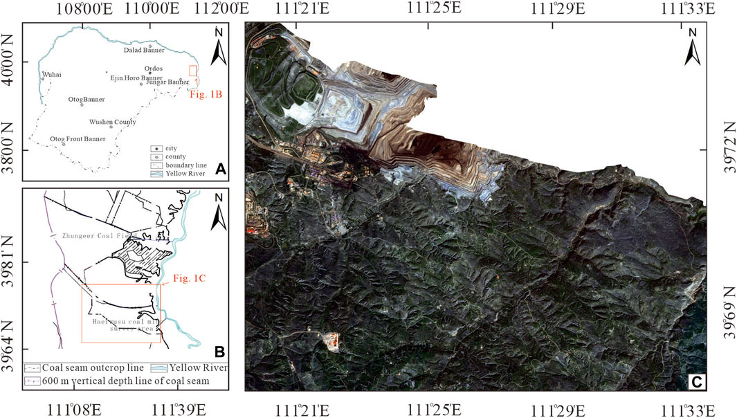
Figure 1. Geographical location map of Haerwusu coal mine in Inner Mongolia Autonomous Region, China. (A) Geographical location map of Jungar coalfield. (B) Geographical location of the Haerwusu mine area. (C) Remote sensing image map of the mine area in 2022.
2.2 Data sources and processing
2.2.1 Remote sensing data
Four periods of remote image sensing—2007, 2012, 2017, and 2022—covered the early stage of coal mining and the period of coal mine ecological management to the present in the study area, including QuickBird data in July 2007 (https://earth.esa.int/) and August 2012 (https://earth.esa.int/), WorldView data in August 2017 (https://earth.esa.int/), and Jilin-1 satellite data in September 2022 (https://www.jl1mall.com), with resolutions of 0.6 m, 0.5 m, and 0.8 m, respectively. We used ENVI 5.3 software to pre-process remote sensing data, including radiometric calibration, atmospheric radiation correction, and geometric and other operations (Jia et al., 2014). To guarantee that the images from various periods were of the same resolution, a nearest-neighbor resampling method was applied to resample the remote sensing images in 2007, 2012, 2017, and 2022 to 10 m using ArcGIS 10.2 software (Seidel et al., 2018). The type of land use was classified into nine categories—cropland, forest, grassland, water, mining land, industrial land, transportation land, and reclaimed and unreclaimed dump—with four sub-categories—forest-grassland, residential land, cropland, and industrial land. The accuracy was more than 85% and the kappa coefficients greater than 0.75 by manual visual interpretation, meeting the requirements for practical applications (Wan et al., 2015). Vegetation index is a straightforward and effective parameter for characterizing the cover and growth of vegetation on the ground surface and is closely related to carbon storage (Zeng et al., 2014). The vegetation indices which employed in the present study are listed in Table 1.
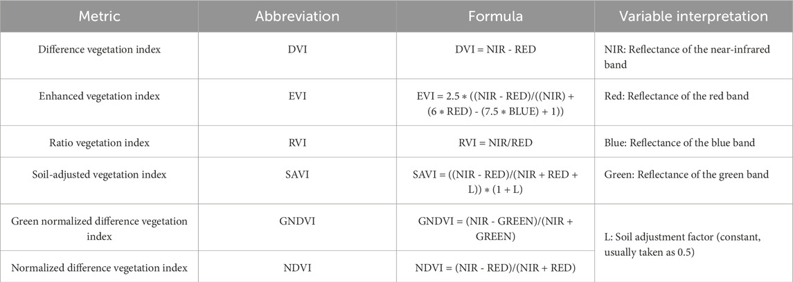
Table 1. Jilin-derived spectral vegetation indices.
2.2.2 Climate data
Temperature and precipitation have significant effects on the distribution pattern of carbon storage (Liu Y. et al., 2022). Mean annual temperature (MAT) and mean annual precipitation (MAP) data in different geographical locations in the study area for 2007, 2012, 2017, and 2022 were obtained from the Resource and Environment Data Center of the Chinese Academy of Sciences (https://www.resdc.cn/ (approved for access on 15 January 2023)) with a resolution of 1,000 m and resampled to 10 m to maintain consistent resolution.
2.2.3 Topographic data
Topographic variables, including elevation (DEM), slope, and aspect, are among the most commonly used predictor variables to predict carbon storage (Wang et al., 2018). The DEM data were derived from the National Aeronautics and Space Administration (NASA) in 2015, which were extracted by SRTM data at 30 m spatial resolution (https://search.earthdata.nasa.gov). On the basis of the DEM, the Space Analyst tool of ArcGIS 10.2 software was used to obtain slope and slope direction data with a resolution of 30. To maintain a consistent resolution for all data, we resampled the topographic data to 10 m.
2.2.4 Landscape pattern index data
The landscape pattern indices for the selected landscape level are shown in Table 2, where their ecological meanings are also presented (Mcgarigal, 2002). Due to the realities of the study area, the resolution has an influence on the accuracy of the results and the simplicity of the calculations. Therefore, we resampled the data to 10 m with the nearest-neighbor resampling method; on this basis, the landscape pattern index was analyzed.
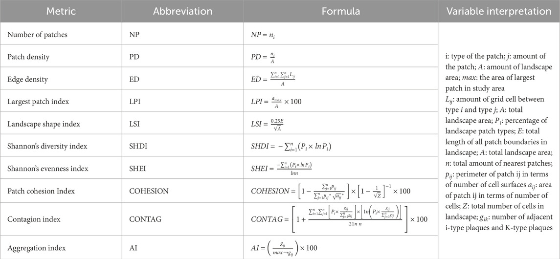
Table 2. Selected landscape pattern indices.
To comprehensively explore the evolution of landscape pattern characteristics in the study area during different periods of time, 10 landscape indices were selected: number of patches (NP), patch density (PD), edge density (ED), patch cohesion index (COHESION), landscape shape index (LSI), Shannon’s diversity index (SHDI), Shannon’s evenness index (SHEI), largest patch index (LPI), landscape contagion index (CONTAG), and aggregation index (AI). To better characterize the spatial distribution information on landscape patter, we used moving window tools to calculate the landscape index in 2022. We analyzed the optimal amplitude and granularity level of the landscape pattern using the moving window tools in Fragstats 4.2 software before calculating the landscape pattern index. The grid distribution of each landscape index was obtained by setting the radius of movement to 30 m, 50 m, 100 m, 150 m, 200 m, and 250 m, respectively, taking multiples of 10 m. Considering the types of indicators and relevance of different landscape pattern indices, we chose the four indicators SHEI, PD, AI, and LSI to judge the moving window radius size. We used GS+ 9.0 software to calculate the semi-variance function of these four indicators which is an important part of geostatistical analyses (Matheron, 1963; Smith et al., 2009), and the appropriate moving window size was selected by observing the Nugget/sill ratio change with different moving window radiuses. The Nugget/sill ratio tended to be stable in the range of 50 m, indicating that the scale is capable of reflecting the spatial variability at the scale inherent in the changing landscape patterns of the region, accompanied by low spatial variation, significant spatial auto-correlation, and little randomness. Therefore, we used images which have been resampled to 10-m resolution for landscape pattern analysis.
2.3 Methods
2.3.1 InVEST model
The InVEST model is a reliable technique commonly used to quantify the regional carbon storage for each LULC type; it assumes that any change in carbon storage is based on LULC changes (Maanan et al., 2019; Liang et al., 2021; Zhu et al., 2022). We calculated the carbon concentration of each grid cell in the study area based on the carbon stored in the four basic carbon pools for each LULC type, which considers above-ground (Cabove) and below-ground carbon concentration (Cbelow), soil organic carbon (Csoil), and dead organic matter (Cdead) (Sharp et al., 2015). Cabove, Cbelow, Csoil, Cdead, and LULC data are the basic input data for estimating the amount of carbon storage in each grid cell (Zhu et al., 2022), and previous studies have found that the impact of LULC changes on carbon storage changes can still be well-assessed whether or not changes in carbon density are taken into account (Zhu et al., 2019; Li et al., 2021). The data for carbon density in this study area are listed in Table 3, and the final calculation can be expressed as Eqs 1, 2.
where i denotes a certain LULC type, Ci denotes the carbon density of LULC type i, C denotes the carbon storage of LULC type i in a given cell, and Si denotes the area of LULC type i.
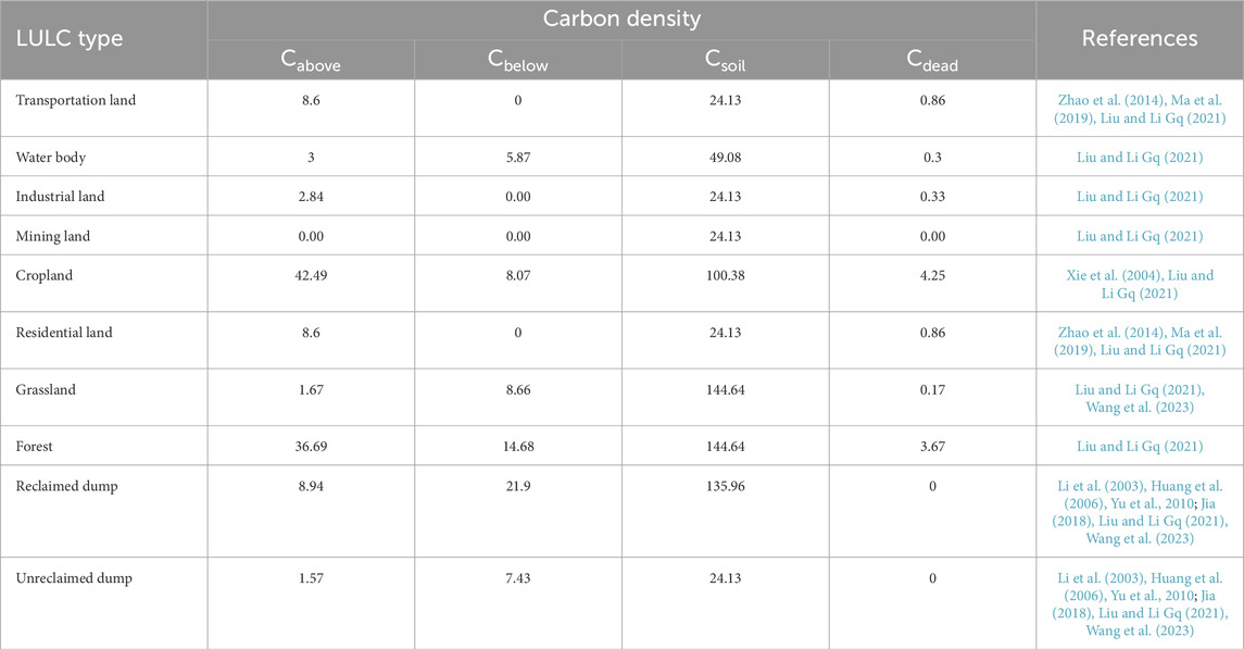
Table 3. Carbon density of LULC types in mining area (t/hm2).
2.3.2 Semi-variance function model
The semi-variance function is key to studying spatial variability, which can reflect the spatial correlation between a sampling point and its neighboring samples. The kriging spatial interpolation can be used in optimal models (Li et al., 2014; Zhao et al., 2017). The semi-variance model is based on the principle that the extent of variability of a pattern and process over small sample point intervals is not significant due to spatial autocorrelation. It considers the magnitude of the statistical correlation coefficients as a function of the distance from the sample; as the distance from the sample increases, the value of the function increases and gradually stabilizes (Li et al., 2014). In the context of moving-window calculations, the semi-variance function can assist in determining the optimal window size to capture sufficient spatial variability in the analysis while avoiding noise introduced by over-refinement. The calculation formula is obtained by Eq. 3.
where N(h) denotes the number of data pairs separated by h; Z (xi) denotes the regionalized variable of the xi position, and N(h) denotes the semi-variance function of the lag distance h between the observations Z (xi) and Z (xi + h).
2.3.3 Correlation analysis and multiple regression model
A 2022 study of the relationship between carbon storage and influencing factors utilized SPSS software (https://www.ibm.com/analytics/spss) to analyze the factors affecting carbon storage. The analysis process was divided into two main stages: correlation analysis and multiple regression modeling.
During the correlation analysis phase, we employed correlation analysis methods to investigate the linear relationships between various factors and carbon storage (SOC). Pearson’s correlation coefficient (r) was calculated to quantify the correlation between SOC and factors such as topographic factors, climate factors, vegetation indices, and landscape pattern indices. The resulting correlation matrix helped identify factors significantly related to carbon storage, providing a foundation for subsequent predictive modeling. The formula for calculating the Pearson correlation coefficient is obtained by using Eq. 4.
where r is the Pearson correlation coefficient; xi and yi are the observed values of the two variables, respectively;
At the stage of multiple regression modeling, based on the results of the correlation analysis, we constructed a multiple regression model to predict SOC. This model underwent significance testing, multicollinearity testing, residual analysis, and heteroscedasticity testing and was required to have a high degree of model fit. Initially, to mitigate the impact of multicollinearity among the independent variables, we conducted a multicollinearity test by calculating the variance inflation factors (VIFs) for all predictors. The predictor with the highest VIF score was removed, and the VIF scores for the remaining predictors were recalculated. This process was repeated until all VIF scores for the independent variables were less than 10, with a stricter standard set to control VIFs below 5. Subsequently, the remaining independent variables were fitted against SOC to obtain the regression model. R squared and adjusted R squared in the results reflect the extent to which the independent variables explain the variance of the dependent variable. Generally, an R squared value above 0.2 is considered good, with a higher R squared value indicating greater model accuracy. A close proximity between adjusted R squared and R squared suggests a stable model. In the significance test, the significance of each predictor was assessed using a t-test with a p-value threshold of less than 0.05, ensuring that the variables included in the model have statistical significance. In the residual analysis, the normality of the model residuals was checked; residuals should be approximately normally distributed without any obvious patterns or trends. In the heteroscedasticity test, the Durbin–Watson test was used to detect heteroscedasticity in the residuals. A Durbin–Watson test value close to 2 indicates constant variance of the residuals.
2.3.4 The coupling coordination degree model
The degree of coupling reflects the degree of interdependence and interconnection of multiple systems (Li et al., 2022). The optimization of the landscape pattern can enhance the regional ecosystem service function, and the forest-land carbon density landscape index can promote each other, reducing the distance between forest-land patches and increasing connectivity, which can mitigate the loss of carbon storage (Shiliang et al., 2019; Tang et al., 2020; Liu X. et al., 2022). The coupling coefficient model was used to calculate the coupling degree of the landscape pattern index, forest and grassland area, and carbon storage, which can be expressed as Eq. 5.
where L denotes the integrated landscape pattern index, F denotes the standardized forest and grassland area, Ca denotes the standardized ecosystem carbon storage, and CLMC denotes the coupling degree among landscape pattern index, forest and grassland area, and ecosystem carbon storage, where a higher value indicates greater correlation between the three factors.
Although there are special cases where the degree of coupling does not necessarily indicate the degree of coordination of a complex system, it may be that there is a very low level of development between systems but a high degree of coupling, which will go against the actual situation (Tang et al., 2020). To avoid this case, we constructed the coupling coordination degree model, which can be expressed as Eqs 6, 7.
where DLMC denotes the degree of coupling coordination, a higher value of which indicates greater coordination among the complex systems; TLMC denotes the composite evaluation index of the three factors; αLMC, βLMC, and γLMC are undefined coefficients, the sum of which is 1. Based on previous studies (Ma et al., 2012; Liu Y. et al., 2022), we believed that the construction among the three factors have the same important status, and we assign αLMC, βLMC, and γLMC to 1/3.
2.3.5 Integrated landscape pattern index, forest and grassland area, and ecosystem carbon storage normalization model
We selected 10 landscape-level indices—NP, PD, ED, LPI, LSI, SHDI, SHEI, COHRSION, CONTAG, and AI—which can well-reflect the degree of aggregation, fragmentation, and connectivity that characterize the mining landscape to calculate the integrated landscape pattern index. Based on previous studies (Shiliang et al., 2019; Liu X. et al., 2022), we applied a normalization technique to make each landscape index dimensionless. The entropy weighting method was used to calculate the weights of the indicators, and then the weights were summed to obtain the integrated landscape index. This can be expressed as Eqs 8, 9
where ωi denotes the entropy weight of the degree of landscape level index k, Lʹ ki denotes the value of standardized landscape level index i in year k, Lki denotes the unnormalized actual value of landscape level index i in year k, and Lmin and Lmax denote the minimum and maximum values of landscape level index i, respectively.
The values of forest and grassland area and ecosystem carbon storage are based on the extreme difference method. The calculation formulas are obatained by using Eqs 10, 11.
where Fi and Ci denote the unnormalized actual values of forest and grassland area and ecosystem carbon storage of year i, and Fmin, Fmax, Cmin, and Cmax denote the minimum and maximum values of forest and grassland area and ecosystem carbon storage, respectively.
2.3.6 Contribution rate of the landscape ecological function
The impact of open-pit mining on mining areas is bound to spread to the surrounding areas of the mining landscape, and the key to exploring the impact is to define the scope of spatial disturbance (Wu et al., 2020). We used the landscape ecological function contribution ratio to quantify the degree of influence of mining activities on the regional carbon storage content using the following calculation formula (Eq. 12):
where Kl denotes the contribution of landscape ecological functions within a distance of l (l = 1, 2, ., n km) from the extent of the mining landscape, including mining districts, dump sites, and other mining land, Cmine denotes the sum of the carbon storage from all the mining landscape, Cl denotes the sum of the carbon storage within l km of the mining landscape, Smine denotes the area of the mining landscape, and Sl denotes the area of the region within l km of the mining landscape.
In summary, the research methodology of the paper is threefold, as shown in Figure 2. The first part is the temporal analysis of carbon storage in the study area based on the InVEST model. The next step is the landscape pattern analysis based on the semi-variance function model and moving-window tools. The final step is based on the coupling coordination degree model, normalization model, and contribution rate of landscape ecological function to explore the correlation between carbon storage, landscape patterns, LULC types, and other environmental factors.
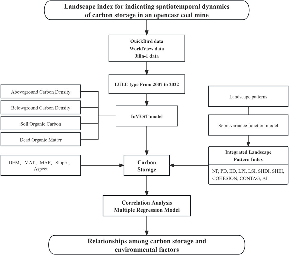
Figure 2. Flowchart of this study’s methodology.
3 Results
3.1 LULC characteristics
3.1.1 LULC distribution
Spatially, the distributions of LULC types in the study area of the different years are obviously different and are determined by human activities, as shown in Figure 3. Grassland and forest had the most wide coverage; cropland and residential lands were primarily in the center of the study area; mining, industrial, and transportational lands, and reclaimed and unreclaimed dumps were primarily observed in the northwest part of the study area; water was not obvious and just existed in 2007.
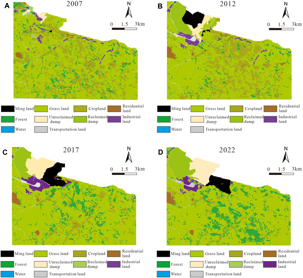
Figure 3. LULC distribution of the study area from 2007 to 2022: (A) 2007, (B) 2012, (C) 2017, and (D) 2022.
Grassland was the largest LULC type, accounting for 60.75%–67.73% of the total area with the maximum value in 2007 and the minimum value in 2012. This is followed by cropland, forest, reclaimed dump, unreclaimed dump, mining land, and industrial land, accounting for 3.30%–21.23%, 4.29%–13.62%, 0.72%–6.12%, 0.83%–5.29%, 0.05%–3.77%, and 1.70%–2.71% of the total area, respectively (Figure 4). Transportation land and water were the relatively lowest LULC types, accounting for 0.23%–0.98% and 0.09%–0.14% of the total area, respectively (Figure 4).
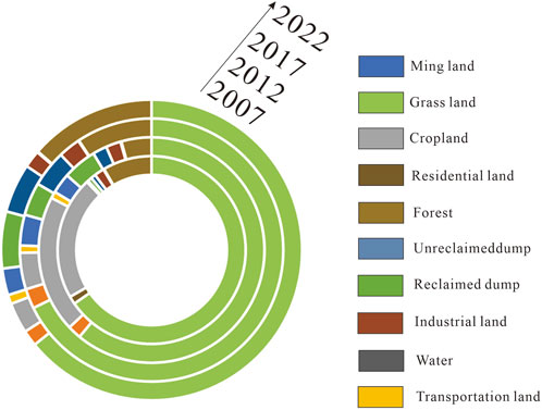
Figure 4. Changes of the LULC structure in the study area from 2007 to 2022.
3.1.2 LULC change
To more clearly describe the fluidity and variety of LULC changes, we used the chord diagram to quantify the transformational relationships between LULC types from different periods in Figure 5. The transfer of LULC types from 2007 to 2022 are listed in Table 4. The results show a clear shift in LULC types, with grassland the dominant contributor to the change in all LULC types, with 18.65 km2 transferred to other land types and accounting for 27.44% of those diversions being the most pronounced from 2007 to 2012 (Figure 5A), and 17.42 km2 transferred in. Cropland was the largest LULC type to be transferred out, with the area amounting to 20.27 km2, accounting for 91.78%, most obvious from 2012 to 2017 (Figure 5B), while only 1.61 km2 was transferred in. The area of water transferred out (0.11 km2) was larger than that transferred in (0.09 km2). The area of forest and reclaimed dump were the major LULC types being transferred in (Figures 5B, C), with areas of 11.02 km2 and 5.84 km2, respectively, which were mainly from grassland and cropland, and 5.62 km2 and 0.22 km2 were transferred out, respectively. Similarly, the area of industrial land, residential land, unreclaimed dump, and mining land transferred in (1.82, 1.30, 4.97, and 2.99 km2, respectively) was larger than that transferred out (1.67, 0.92, 0.34, and 0.51 km2).
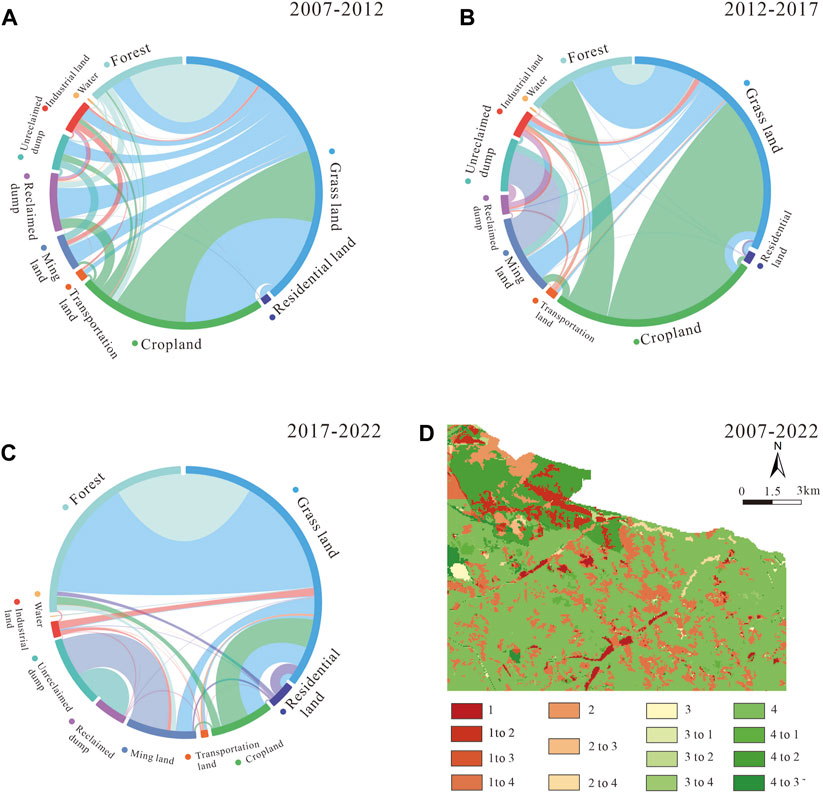
Figure 5. LULC transfers chord diagram. (A) 2007–2012, (B) 2012–2017, (C) 2017–2022, and (D) LULC change characteristics map 2007–2022.
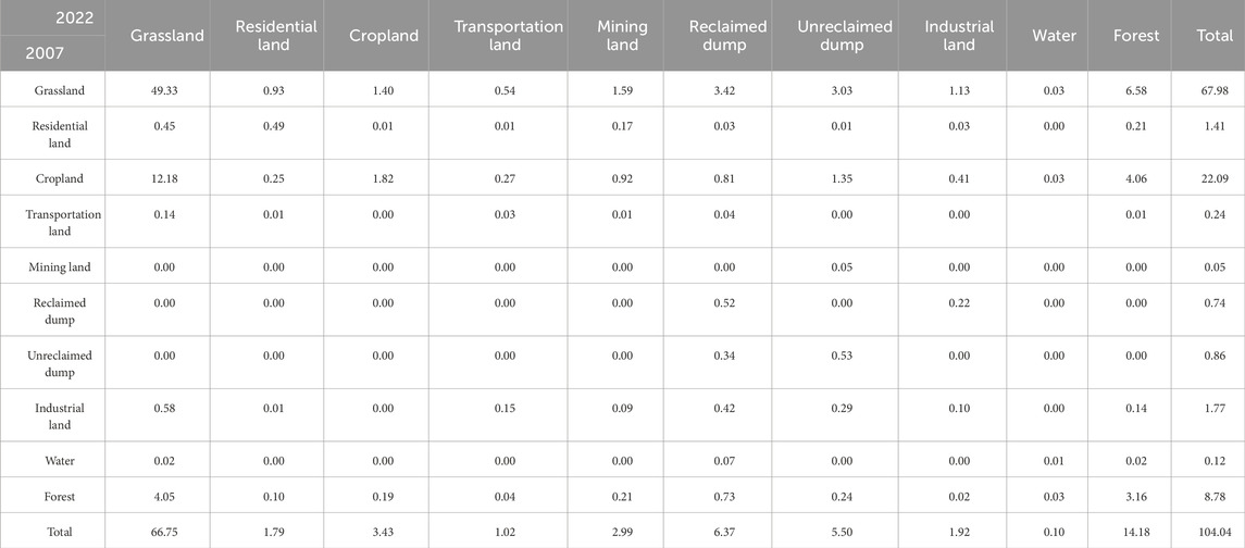
Table 4. Transfer matrix of LULC changes in the mining area 2007–2022 (km2).
In order to better visually reflect the impacts of human activities on LULC type from 2007 to 2022, nine LULC types were classified according to their characteristics as forest-grassland, cropland, residential land, and industrial land as anthropogenic activities on land type (Figure 5D). Forest-grassland converted to industrial land was primarily concentrated in the northwest parts of the study area (10.37 km2), cropland was scattered in the south (1.59 km2), and residential land was more dispersed (1.64 km2). Cropland was mostly converted to forest-grassland, which was widely distributed in the center and east of the study area (16.25 km2), while the north-west of the cropland was converted to industrial land (3.48 km2), and scattered cropland in the central areas was converted to residential land (0.54 km2). Similarly, residential land converted to forest-grassland was also scattered in the central and east of the study area (0.85 km2), to industrial land was concentrated in the northwest areas (0.36 km2), and to cropland was scattered in the whole study area (0.02 km2). The area of industrial land transferred out was insignificant, with only localized conversion of small areas into residential land and forest-grassland (0.15 and 0.71 km2). The results showed that an inter-transformation existed between all the LULC types, although the main manifestation was the transformation from cropland to forest-grassland and industrial land.
3.2 Carbon storage characteristics
3.2.1 Carbon storage change
The carbon storage values for the study area are presented in Table 5, with total carbon storage of 159.95 × 10⁴, 150.85 × 10⁴, 147.51 × 10⁴, and 151.91 × 10⁴ t in 2007, 2012, 2017, and 2022, respectively, using the InVEST model. The results showed a fluctuation in the value of carbon storage from 2007 to 2022, with a gradual decrease from 2007 to 2017 and an increase after 2017. The largest value of carbon storage was in 2007, with a smaller area of industrial land and a larger area of grassland, forest, and cropland with high carbon density than other years. From 2007 to 2017, carbon storage decreased at a rate 1.24 × 10⁴ t/yr, with a cumulative loss of 12.44 × 10⁴ t; a sharp decline occurred from 2007 to 2012, manifested as a shift conversion from grassland and forest into mining land, dump, and industrial land. From 2017 to 2022, there was an increase in the total carbon storage in the study area by 4.39 × 10⁴ t, with the area of forest and reclaimed dump increasing. Thus, from 2007 to 2017, the conversion of LULC was mainly from high to low carbon density land, and, from 2017 to 2022, land type with low carbon density was converted to land types with high carbon density.
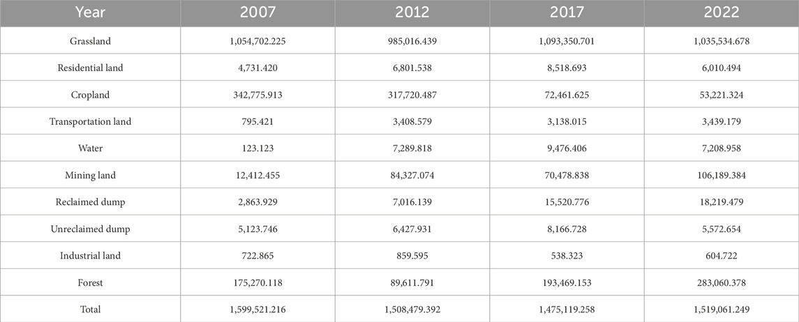
Table 5. Carbon storage of different LULC types in the mining area from 2007 to 2022 (t).
3.2.2 Carbon storage spatial distribution dynamic
Carbon density spatial variability is shown in Figure 6. From 2007 to 2012, the variation in carbon storage was primarily concentrated in the northwest of the study area, ranging from −175.55 to 170.68 t/hm2 and increases and decreases in areas of 19.69 km2 and 12.83 km2, accounting for 18.92% and 12.33%, respectively (Figure 7A). Meanwhile, 68.75% of the region’s carbon storage remained unchanged. From 2012 to 2017, carbon storage in the northern parts of the region changed obviously, with changes ranging from −175.55 to 170.68 t/hm2. An upward trend was shown in 11.57% of the areas, 19.87% of the areas had a downward trend, and 68.56% of the areas remained unchanged (Figure 7B). During 2017–2022, carbon storage changed considerably across the study area, with increases concentrated in the north and middle of the study area, ranging from 0 to 170.68 t/hm2, and declines were also concentrated in the middle of the study area, ranging from −175.55 to 0 t/hm2—17.63% and 9.80% of the areas (Figure 7C). Additionally, 72.57% of the areas remained unchanged. Hence, the carbon storage showed little spatial variation in the study area over 2007–2022, with 53.85% of the areas remaining unchanged, 27.58% of the areas trending downward, and 18.56% of the area trending upward (Figure 7D).
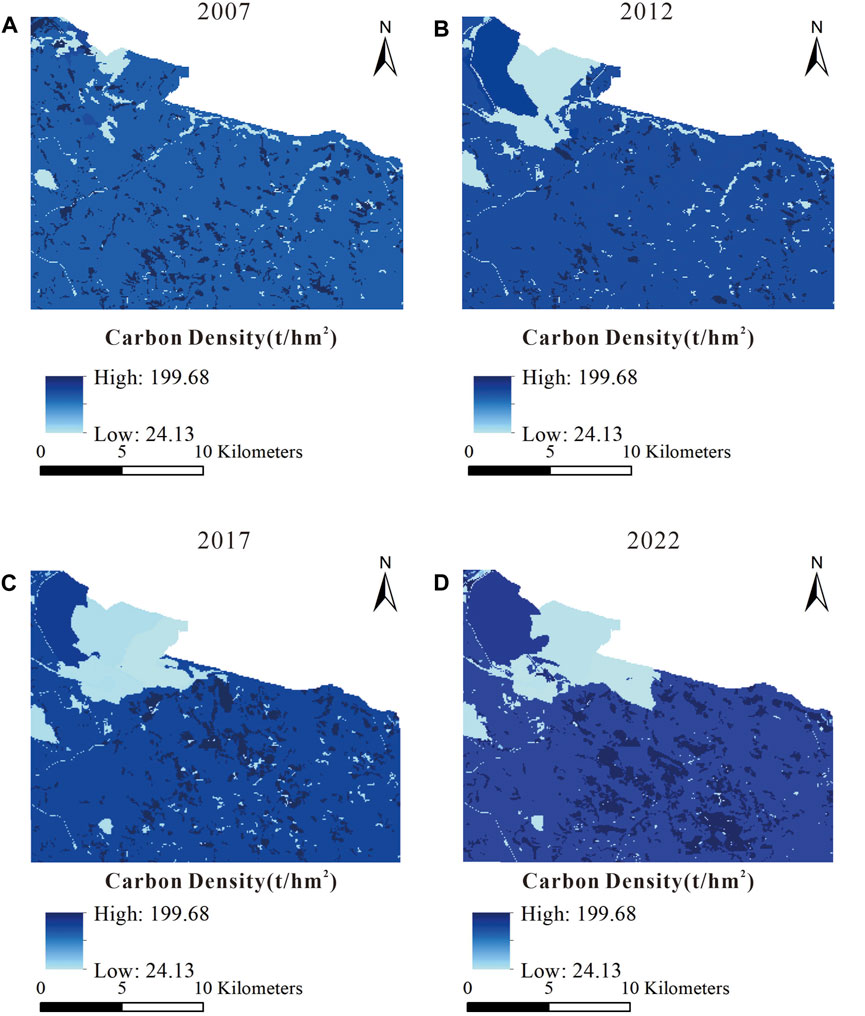
Figure 6. Carbon storage distribution of the study area from 2007 to 2022: (A) 2007, (B) 2012, (C) 2017, (D) 2022.
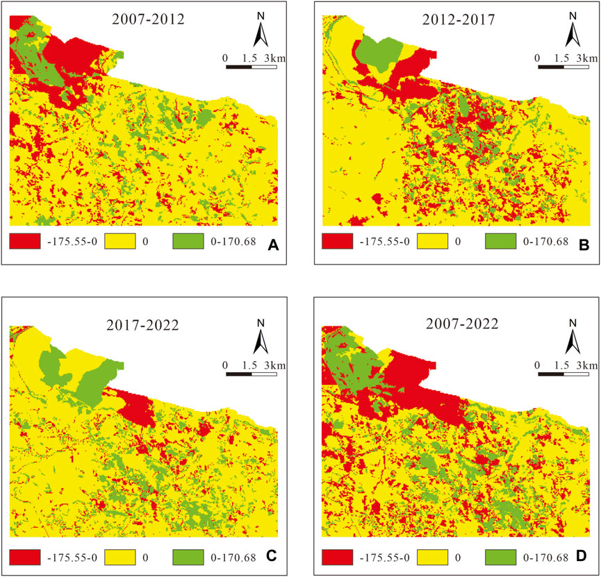
Figure 7. Spatial distribution of carbon storage in the study area from 2007 to 2022: (A) 2007–2012, (B) 2012–2017, (C) 2017–2022, and (D) 2007–2022.
3.3 Landscape pattern characteristics
3.3.1 Landscape level change characteristics
The landscape pattern index of landscape level reflects the landscape pattern across the study area (Wu et al., 2012). As shown in Table 6, all landscape pattern indices have changed with a certain amount of fluctuation from 2007 to 2022. To better analyze the relationship between landscape patterns, LULC type, and carbon storage, we created an integrated landscape index. To avoid errors caused by excessive landscape pattern factors involved in calculating the composite landscape pattern index combined with the results of the previous study, we chose six landscape pattern indices with representative types for the calculation: NP, PD, LSI, COHESION, SHDI, and SHEI (Liu Y. et al., 2022). Their values changed with a certain amount of fluctuation from 2007 to 2022 (Table 6). Based on the polarization and entropy weight method, the weighting values of each landscape pattern index are 0.173, 0.172, 0.227, 0.193, 0.117, and 0.118. Thus, the integrated landscape index values in 2007, 2012, 2017, and 2022 are 0.614, 0.519, 0.449, and 0.506, respectively (Table 6). The changes of the integrated landscape index values for 2007–2022 indicate that the patches of the mining landscape are progressively more discrete and increasingly fragmented from 2007 to 2017 and that the situation began to improve after 2017, with patches becoming more cohesive and less fragmented. The above calculations were performed on Python V 3.9.0.

Table 6. Four-year landscape pattern indices.
3.3.2 Spatial variability of landscape level in 2022
Comparing each landscape pattern index value in 2007, 2012, 2017, and 2022, the landscape pattern characteristics in 2022 are more typical, which can visually reflect the information about landscape pattern. Figure 8 shows the spatial distribution of 10 landscape pattern indices within the study area. The spatial distribution characteristics of COHESION, AI, and LPI were similar, where the high-value areas occupied a large part of the region with a maximum value of 100. The high-value areas were located around the edges of the study area, especially in areas such as mining land and dump sites, while the low-value areas were in the in the central part of the study area, where the LULC types were dominated by forest and grassland. In general, the values of COHESION, AI, and LPI got lower from the border to the central area.
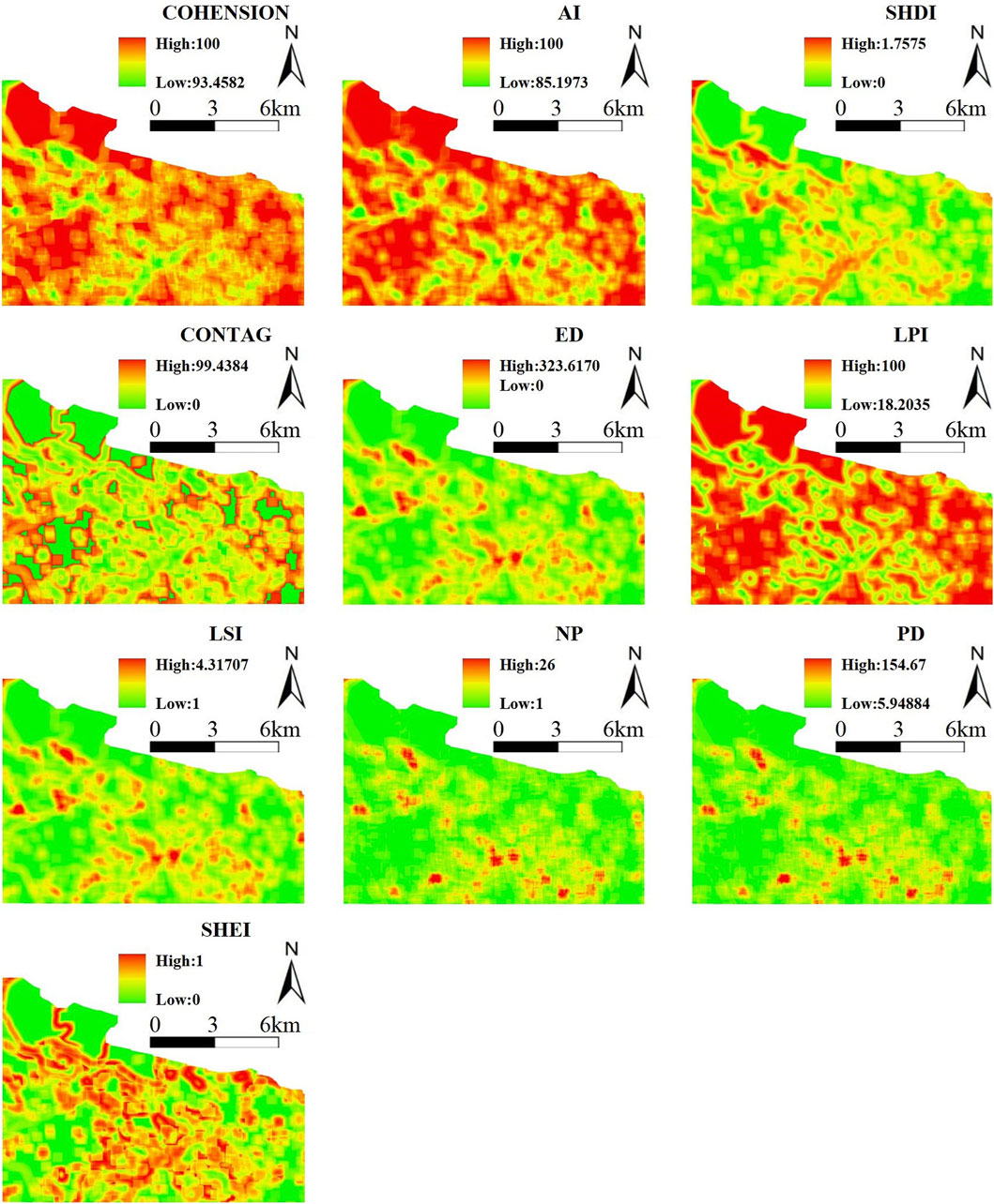
Figure 8. Spatial distribution of landscape pattern indices in 2022.
CONTAG, SHDI, and SHEI showed similar characteristics, and the distribution varied greatly: the low value of 0 areas were primarily distributed in areas with concentrations of human activities such as mining land and dump sites, while, in the central part of the region, values varied greatly and were not concentrated. The overall distribution of ED, LSI, NP, and PD was similar, where the distribution of low-value areas were in the border region, and the high-value areas were located in central and southern regions with a wide range of values.
3.4 Relationships between carbon storage and influencing factors in 2022
In a comprehensive analysis, the carbon density values were found to be correlated with topographic factors, climate factors, vegetation indices, and landscape pattern indices. Among the topographic factors, carbon density was significantly and positively correlated with DEM (r = 0.258) (p < 0.01), while the correlation with slope and slope direction was not significant. In terms of climate factors, carbon density exhibited a significant positive correlation with MAP (r = 0.264) (p < 0.01) and a significant negative correlation with MAT (r = −0.217) (p < 0.01). For the vegetation index data, carbon density was significantly positively correlated with EVI (r = 0.130), RVI (r = 0.513), SAVI (r = 0.585), GNDVI (r = 0.402), and NDVI (r = 0.584) (p < 0.01) and significantly negatively correlated with DVI (r = −0.343) (p < 0.01). For landscape pattern indices, carbon density showed significant negative correlations with LPI (r = −0.108), COHES (r = −0.009), CONTAG (r = −0.024), and AI (r = −0.111) (p < 0.01). A significant positive relationship was observed between carbon density and SHEI (r = 0.149) (p < 0.01). Carbon density was also positively correlated with LSI (r = 0.091) and ED (r = 0.091) (p < 0.05). The correlation between carbon density and NP, SHDI, and PD was not significant (Table 7).
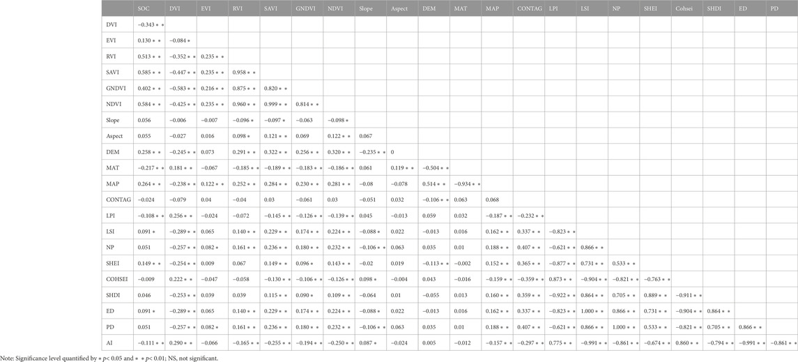
Table 7. Correlation coefficient between carbon storage and environmental and landscape factors.
Taking into consideration the correlations with carbon density values, this study established a regression equation of carbon density, constructed a multi-regression model linking each influential factor to carbon density content, and analyzed the contribution of each factor to the change of carbon density. Supplementary Table S1 shows details of the data used in the regression analysis.
For topographic factors, climate, and vegetation index factors, SAVI, GNDV, DEM, and MAT data were included in the model. Other data (such as MAP data) were excluded due to failing the multicollinearity test or having better alternative options within the same category of factors. The residual and standard residual means of the regression equation were both 0, and the Durbin–Watson test value was 1.572, meeting the independence condition (Table 8). Variance inflation factor (VIF) values were all less than 5 (Supplementary Table S2), meeting the collinearity test. Supplementary Table S3 shows the test for residual normality. The optimal model is as follows:
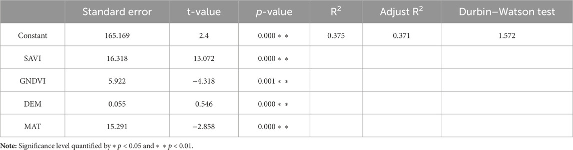
Table 8. Statistical characteristics of coefficients and cross-validation results of Model 1.
From Model 1, it can be observed that SAVI and GNDVI among the vegetation index data and MAT among the climate factors contributed significantly to carbon density.
When considering topographic factors, climate factors, vegetation index data, and landscape index data, SHEI and AI data were included in the model. The residual and standard residual means of the regression equation were both 0, the Durbin–Watson test value was 1.596, meeting the independence condition (Table 9), and VIF values were all less than 5 (Supplementary Table S4), meeting the collinearity test. Supplementary Table S3 shows the test for residual normality. The optimal model is as follows:
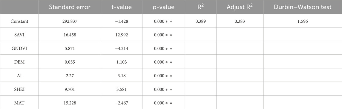
Table 9. Statistical characteristics of coefficients and cross-validation results of Model 2.
From Model 2, it can be observed that, in addition to vegetation indices and climate factors, significant contributors to carbon density are SHEI and AI, which are directly related to landscape patterns.
Combining models 1 and 2, it can be concluded that, together, DVI, EVI, SAVI, GNDVI, DEM, MAT, SHEI, and AI data more reasonably explain the variation in carbon density. The explanation rate was 37.5% (Model 1) when considering only topographic, climate, and vegetation index factors. After adding SHEI and AI data, the explanation rate increased by 1.4% (Model 2).
3.5 Spatial and temporal analyses of landscape ecological functions
The mean value of carbon storage per unit area in the study area from 2007 to 2022 is relatively stable, although it is closely related to spatial variation, which can be divided into two stages (Figure 9). From 0 to 4 km of the mining landscape, Cmean values increased significantly, reflecting the anthropogenic impacts on carbon storage and landscape. Cmean values fluctuated more than 4 km from the mining landscape, indicating that the carbon sequestration capacity of the landscape was less affected by human activities such as mining but directly by landscape type. The results demonstrate that human activities affect the ecological system functions in a certain distance which will disturb regional ecosystem conditions; outside of that distance, the impact on regional ecological function was not related to the distance, consistent with previous studies (Wu et al., 2020).
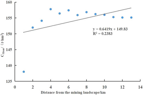
Figure 9. Mean value of carbon storage per unit area in the study area from 2007 to 2022.
As Figure 10 shows, increasing of the area of the mining landscape increases Kl, in which Kl in the range of 0–1 km at the beginning of mining in 2007 was only 46.67%, indicating that the influence of human activities on the regional carbon storage was insignificant when human activities were weak, and gradually increased with increased human activities. Furthermore, the Kl in different buffers had a similar change in 2007, 2012, 2017, and 2022. The Kl values for 0–4 km decreased rapidly with the value of 0.0104, 0.359, 0.0583, and 0.0514, respectively, indicating a significant influence of human activities for landscape ecological function. The values of Kl for 4–8 km decreased slowly, with rates of 0.0040, 0.0069, 0.0075, and 0.0111, respectively, indicating that the negative impacts of mining activities are still rapidly diminishing. Beyond 8 km, Kl tends to be stable, indicating a weak influence on landscape ecology. Thus, the above analysis shows that the Kl value of the buffer zone is larger the closer it is to the mining landscape, and the area within 4 km is the main disturbed area; however, the impacts continue to diminish in the area between 4 and 8 km, and the area beyond 8 km suffers very little or even negligible disturbance.
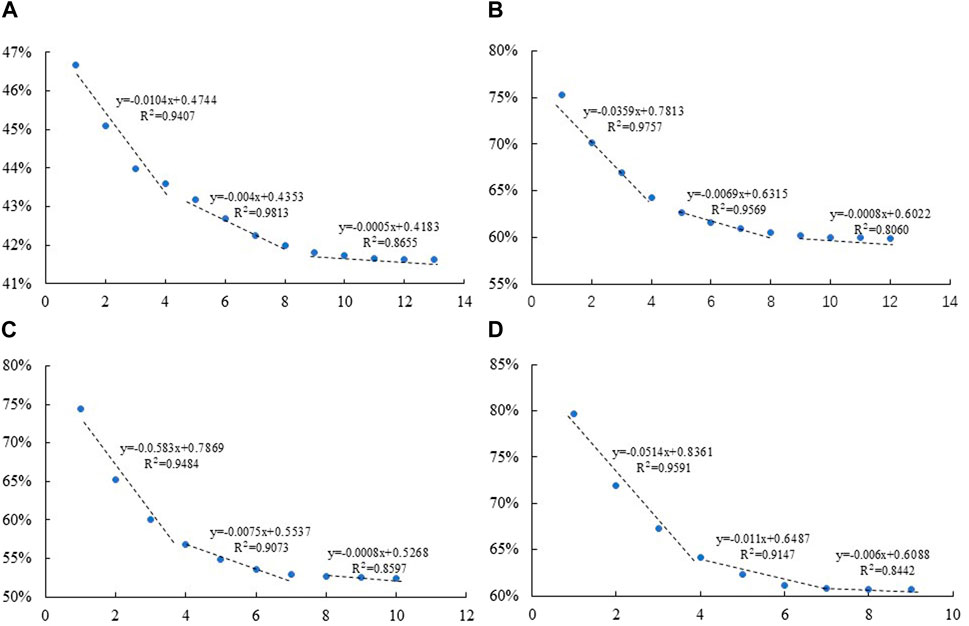
Figure 10. Landscape ecological function contribution ratio in different buffer zones from 2007 to 2022: (A) 2007, (B) 2012, (C) 2017, and (D) 2022.
4 Discussion
4.1 Effects of LULC dynamic changes on carbon storage and landscape pattern
The application of the InVEST model to land-use change to calculate carbon stock changes over time for each map cell indicates that the calculation of the carbon storage in this study directly depends on LULC dynamic changes. Landscape patterns, as the end result of the interaction of natural and human activity elements at complex spatio-temporal scales, have always been the most direct manifestation of LULC change (Wang et al., 2022; Wang et al., 2022;Liu et al., 2023), and the landscape pattern index can provide deep information on the LULC change and influence the evolution of the ecological effects (Moser et al., 2002; Zhang et al., 2021). Therefore, the spatio-temporal distribution and change characteristics of carbon storage and landscape patterns were obtained from the LULC dynamic changes.
As a nationally important energy and heavy chemical industry base, Jungar county’s coal industry accounts for more than 70% of its total economy. Haerwusu coal mine, which is considered the largest coal production unit in China, provides considerable economic support to Jungar county. Its raw coal output has been climbing from the early stage of mining, and the raw coal production of each year has reached 21.68 × 10⁶ t. The coal reserves of the mining area exceed 17 × 108 t. with a recent annual raw output of 31 × 106 t (Li et al., 2020). As the scale of mining activity in coal mines has increased each year, areas of industrial land have continued to increase. In particular, similar trends were observed for mining land areas and industrial land areas, with a gradually increasing trend from 2007 to 2017 and a decreasing trend since 2017. The main reason for the changes in mining land and industrial land was that, during the early stage, there was a rapid increase in the area of industrial and mining land due to the needs of enterprise development. The Haerwusu coal mine was evaluated as a national green mine pilot unit in 2014. Zhuneng Group adopted a new synergistic development model combining mining with land reclamation, including green mining, reclamation and greening, development of modern agriculture and animal husbandry, and construction of mine parks, leading to a subsequent decline in the area of mining area and industrial land.
The variations in forest and grassland areas fluctuated significantly, with a 17.48% decrease over the study area from 2007 to 2012 during the early stage of mining and then have sharply increasing since 2012, with an increasing proportion of forest. This is principally due to the following reasons. 1) During the beginning of coal mining, the coal mining damage and land reclamation implementation caused the main damage to the forest and grassland as raw coal production increased and coal mining expanded. 2) From 2012 to 2022, with a great investment in ecological management by the Zhuneng Group, vegetation coverage in the mining area continuously improved; in 2022, the vegetation coverage accounted for approximately 70% of the Haerwusu mining area. 3) With the “Conversion of Cropland to Forest and Grassland” policy continuing to be implemented, the cropland was turned into forest and grassland (Zhang et al., 2020). The area of cropland remained stable from 2007 to 2012 and has decreased significantly since then. The reasons for the variation of cropland area are as follows. 1) For opencast mining coal mines, various and sustained forms of land destruction, including mining, excavation damage, and occupancy, were the main reasons for loss of cropland (Cao et al., 2011), and the direction of land damage also reinforced the decrease of cropland and residential land. 2) To obtain more compensation from opencast mines, a number of farmers planted trees or built houses on cropland, prompting the conversion of cropland into forest and construction land in a short period of time (Zhang et al., 2020). 3) The implementation of the “Conversion of Cropland to Forest and Grassland” policy has further exacerbated the loss of cropland (Cao et al., 2014). Similarly, for residential land in the study area, a significant decrease has occurred since 2017, mainly caused by the continuing urbanization from more residents relocating and congregating in towns and cities from original landforms. Furthermore, coal mining and land reclamation also occupied the residential land, causing its variation.
4.2 Relationships between carbon storage and environmental factors
Previous studies have shown that vegetation indices are useful in explaining the variability and distribution of ecosystem carbon storage (Guo et al., 2020; Odebiri et al., 2020; Shi et al., 2021; Wang et al., 2021). Shi et al. (2021) proposed a remote sensing inversion model for above-ground forest carbon storage based on GNDVI as the independent variable, with average relative accuracy of 82.19% . They reported that SAVI played a very important role in the prediction of carbon storage (Wang, 2022). The significant correlations between carbon storage and GNDVI and SAVI can be seen in Table 7 and Figures 11A–C. Terrain factors control the distribution of thermal and water resources and influence the regional distribution of vegetation cover and land use, potentially altering soil organic carbon inputs (Li et al., 2016; Zhao et al., 2017). Liu Y et al. (2022) suggested that ecosystem carbon storage tends to increase with elevation, indicating a positive correlation relationship between ecosystem carbon storage and DEM, which is in line with the results of this study (Liu X. et al., 2022) (Figure 11D). In addition, slope aspect, while altering hydrothermal conditions and vegetation growth, has a smaller effect on carbon density, and the correlation is not significant as it lacks the characteristics of a long-term effect (Chang et al., 2021). Previous studies have demonstrated that human activities such as mining and reclamation have diminished the effects of slope aspect and slope (Li et al., 2016; Liu Y. et al., 2022). Climate has been recognized as an important factor in ecosystem carbon storage. Generally, a strong positive correlation exists between MAP and ecosystem carbon storage, and this can be explained by the fact that precipitation stimulates plant biomass, leading to an increase in ecosystem carbon storage. Furthermore, MAT shows a negative relationship with ecosystem carbon storage, suggesting that higher temperatures can promote the mineralization rate of soil organic matter, leading to a reduction in ecosystem carbon storage (Song et al., 2018; Wang et al., 2019). The relationship of carbon storage with MAP and MAT can be seen in Table 7, and the results of the multicollinearity test indicate that temperature data are more appropriate as a factor to analyze its contributions to carbon ecosystem storage variation (Figure 11E).
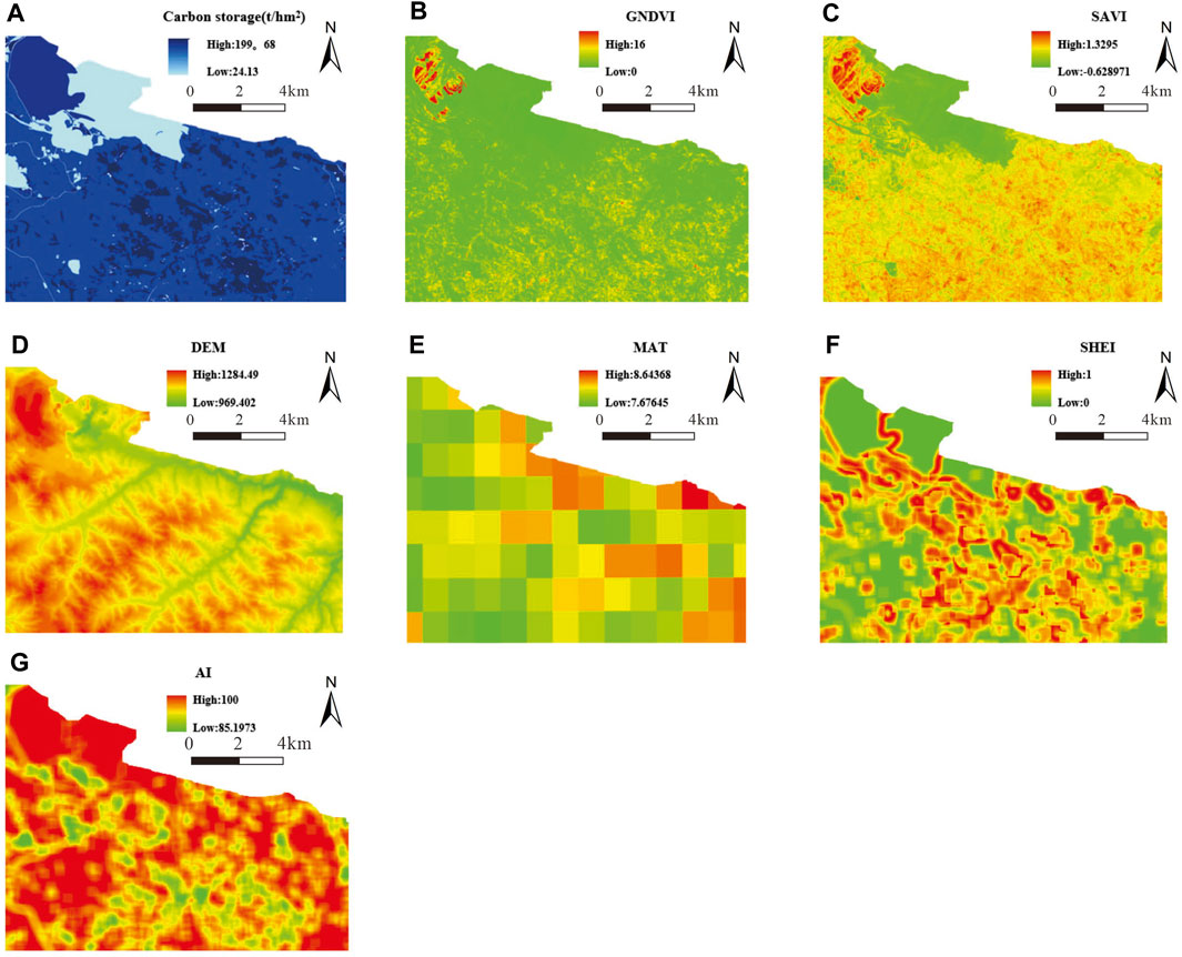
Figure 11. Carbon storage and spatial distribution of factors closely related to carbon storage in 2022. 2. (A) Carbon storage, (B) GNDVI, (C) SAVI, (D) DEM, (E) MAT, (F) SHEI, and (G) AI.
Landscape patterns have a direct relationship with ecosystem carbon storage, which is reported by Liu X. et al. (2022). Table 7 shows that SHEI, AI, and LPI were significantly correlated with carbon storage. SHEI, representing the diversity of the landscape types, shows a positive correlation with carbon storage (Figure 11F). A high value for SHEI means a high proportion of some natural landscape areas causing landscape complication, which can better promote material circulation (Fu et al., 2001). AI and LPI, which can describe the degree of clustering and the dominant patch types in the landscape, were both negatively correlated with carbon storage, indicating that a concentrated distribution and the existing dominant landscape are not conducive to carbon storage content. The contiguous concentration of landscape patches will take a certain amount of time, resulting in the destruction of a large quantity of soil agglomerates and accelerating the depletion of soil nutrients—unfavorable to increased ecosystem carbon storage (Carter et al., 2002; Liu Y. et al., 2022). These two indices have a similar impact on carbon storage, and AI is more suitable as a factor for analyzing the contribution to carbon storage within the same category (Figure 11G).
The value of the coupling coordination degree reflects the main influences of its factors (Li et al., 2022). Statistically, the values of forest and grassland area in 2007, 2012, 2017, and 2022 in Haerwusu mining area were 76.76, 67.98, 80.16, and 80.92 km2, respectively. To avoid the extreme values of 0, we used the extreme difference method for forest and grassland area by setting the value of forest and grassland area in 2006 as the minimum value and the value of forest and grassland area in 2023 as the maximum. For the minimum value of ecosystem carbon storage, we used the carbon storage value calculated from the forested land with the largest area of land type. Thus, the degree of coupling coordination value in the study area from 2007 to 2022 was 0.887, 0.720, 0.849, and 0.867, respectively. In 2007, the coupling coordination degree of the mining area was excellent during the mining area in the initial stage of mining, with little interference from anthropogenic activities and a larger proportion of grassland. Since 2007, the mining area has increased dramatically and the grassland area has decreased significantly, while the carbon sequestration system and landscape pattern index were significantly affected by human activities. Until 2012, the degree of coupling coordination was primary, reflecting the serious impact of human activities on the coupling of carbon storage forest and grassland area-landscape pattern index. From 2012 to 2017, with the increase of forest land area and carbon storage and the decrease of integrated landscape index value, the degree of coupling coordination increased well. From 2017 to 2022, as ecological restoration efforts intensified, human activities had a great impact on the coupling coordination degree of carbon storage-forest and grassland area-landscape pattern, resulting in a significant increase in forest land converted from cropland, continuous decrease of integrated landscape index value, and continuous increase of carbon storage. In summary, the carbon storage forest and grassland area-landscape pattern coupling coordination degree weakened and then increased, reaching its lowest point in 2012 and starting to increase thereafter, indicating that the changes in the degree of coupling coordination are greatly affected by human activities.
4.3 Trends in changes of the contribution rate of landscape ecological function
From 2007 to 2022, with the gradual expansion of the mining area, Kl for the same area range changed significantly, with the lowest value in 2007 and variable fluctuation since thereafter. This is mainly due to two factors. 1) At the beginning of mining in 2007, industrial land was dominated by mining land, with a higher proportion of forest and grassland areas containing relatively high carbon density. 2) With continued mining activities after 2007, the investment in ecological management increased significantly, leading to an increased proportion of reclaimed dump among the industrial landscape; its carbon density is significantly high compared to other types of industrial land types, and prominently increases Kl. Kl in the same area range in different years indicates varied economy investment and the effect of ecological management from 2012 to 2022.
In mining areas, the impacts of human activities such as mining on carbon storage are mainly concentrated between 0 and 4 km, while beyond 4 km that tends to be stable. The reasons for the changing characteristics of the impacts are as follows. 1) As shown in Table 3, carbon density is significantly higher in forests and grasslands than in mining landscapes, with the proportion of the former increasing significantly 0–4 km from the mining landscapes; outside of 4 km, little change is seen in the area proportions of each landscape type. 2) Ecological restoration efforts are mainly concentrated in industrial land, such as mining land, dump sites, and surrounding areas. The range 0–4 km from industrial land is the main ecological restoration area; as the distance increases, the proportion of the area occupied by reclaimed dump also increases. Within a 4–8 km range, ecological restoration is also carried out, while human activities still have an impact on regional carbon storage. Beyond 8 km, there is little ecological restoration, and the implications for the carbon storage in the study area are mainly influenced by the natural ecology. As discussed above, we propose that the carbon storage-sensitive areas in the study area are classified into three levels: extremely sensitive areas 0–4 km, sensitive areas 4–8 km, and insensitive areas beyond 8 km—consistent with the results of previous studies.
Previous studies have demonstrated that mining activities have a regular character in terms of the contribution of landscape ecological functions in mining areas. Kang et al. (2014) considered the theoretical reference range for the impacts of the Shengli surface mine on the ecological health of grassland landscapes to be 5 km. Wu et al. (2020) proposed that the mean values of a carbon density buffer zone from a mining landscape of 0–7 km belong to sensitive areas, which is in line with this study (Liu X. et al., 2022). In addition, the value change of the contribution of the landscape ecological functions over years is more closely related to mining and the restoration of coal mines.
4.4 Contributions and limitations
Research on the impact of human activities, such as surface mining, on carbon storage and landscape patterns in mining areas is a large project which requires much validation and in-depth research. Although the relationship between carbon storage and landscape patterns and other factors has been investigated, the contribution rate of landscape ecological function was proposed to analyze the impact of surface mining on coal mines in this study. The paper has some limitations, which can be addressed in future research. 1) Carbon storage was calculated using the Invest model, which is mainly based on LULC and may not accurately reflect the carbon cycle and storage. 2) LULC carbon density data were taken from previous studies and lack field sampling data. They especially do not consider the functional differences in carbon sequestration capacity of different plant types. 3) Surface mining may cause a significant change for surface topography, and different coal seam mining techniques and resource recovery rates will inevitably cause different impacts on the surface (Wu et al., 2020). There i thus a need for comprehensive, real-time, long-term monitoring of open-pit mining conditions and other data. In addition, in real landscapes, the complexity of ecosystems makes it difficult to assess their value (Guo et al., 2021), further affecting the accuracy of the analysis of the correlation between carbon storage and landscape patterns.
5 Conclusion
In this research, we addressed the effects of LULC changes on ecosystem carbon storage and analyzed factors including landscape patterns, vegetation indices, elevation, and temperature that influenced carbon storage in Haerwusu open-pit coal mine from 2007 to 2022. The main conclusions are as follows:
(1) Carbon storage fluctuated from 2007 to 2022, with a gradual decrease from 159.95 × 10⁴ to 147.51 × 10⁴ t over the period 2007–2017 and an increase to 151.91 × 10⁴ t after 2017.
(2) The carbon storage forest and grassland area-landscape pattern coupling coordination degree weakens and then increases, ranging 0.887–0.867, reaching its lowest point of 0.720 in 2012.
(3) Vegetation indices, temperature, and elevation governed the geographical pattern of ecosystem carbon storage, explaining 37.5% of carbon storage spatial variability; the combination of SHEI and AI improved the explanation by 1.4%.
(4) The landscape ecological function contribution ratio from 2007 to 2022 has a similar characteristic, which can classify the carbon storage-sensitive areas of the study area into three levels: extremely sensitive areas ranging 0–4 km, sensitive areas ranging 4–8 km, and insensitive areas beyond 8 km.
Data availability statement
The raw data supporting the conclusion of this article will be made available by the authors, without undue reservation.
Author contributions
MC: data curation, formal analysis, methodology, and writing–original draft. SM: conceptualization, funding acquisition, supervision, validation, and writing–review and editing. XH: data curation, investigation, methodology, and writing–original draft. LC: LC: data curation and writing–original draft. LZ: investigation, visualization, and writing–original draft. HY: investigation and writing–review and editing. RW: methodology, project administration, and writing–original draft. XW: data curation and writing–original draft. YZ: software, validation, and writing–original draft. PZ: investigation, software, and writing–original draft.
Funding
The author(s) declare that financial support was received for the research, authorship, and/or publication of this article. This research was funded by research on biodiversity baseline survey and conservation practice pathways, grant number GJNY-23-2 and Research and Engineering Demonstration on Key Technologies for the Integration and Operation Control of the Entire Industry Chain Enabled by Beidou and Spatial Intelligence, grant number GJNY-24-52.
Conflict of interest
MC, SM LZ, RW, PZ, and XW were employed by the China Energy Digital Intelligence Technology Development (Beijing) Co., Ltd. XH was employed by the China Chengtong Ecological Co., Ltd. HY was employed by China Energy Zhunneng Group Co., Ltd.
The remaining author declares that the research was conducted in the absence of any commercial or financial relationships that could be construed as a potential conflict of interest.
Publisher’s note
All claims expressed in this article are solely those of the authors and do not necessarily represent those of their affiliated organizations, or those of the publisher, the editors, and the reviewers. Any product that may be evaluated in this article, or claim that may be made by its manufacturer, is not guaranteed or endorsed by the publisher.
References
Bian, Z. F., Inyang, H. I., John, D. L., Otto, F., and Struthers, S. (2010). Environmental issues from coal mining and their solutions. Min. Sci. Technol. 20, 215–223. doi:10.1016/s1674-5264(09)60187-3
Cao, Q., Chen, X., Shi, M., and Yao, Y. (2014). Land use/cover changes and main-factor driving forcein Heihe middle reaches. Trans. Chin. Soc. Agric. Eng. 30 (5), 220–227.
Cao, Y., Bai, Z., Zhou, W., and Zhang, X. (2016). Characteristic analysis and pattern evolution on landscape types in typical compound area of mine agriculture urban in Shanxi Province, China. Environ. Earth Sci. 75, 585–615. doi:10.1007/s12665-016-5383-1
Cao, Y., Zhou, W., Wang, J., and Yuan, C. (2011). Spatial-temporal pattern and differences of land use changes in the Three Gorges Reservoir Area of China during 1975–2005. J. Mt. Sci. 8, 551–563. doi:10.1007/s11629-011-2008-8
Carter, M. R., Skjemstad, J. O., and Macewan, R. J. (2002). Comparison of structural stability, carbon fractions and chemistry of krasnozem soils from adjacent forest and pasture areas in south-western Victoria. Soil Res. 40 (2), 283–297. doi:10.1071/sr00106
Chang, M., Meng, S., Zhang, Z., Wang, R., Yin, C., Zhao, Y., et al. (2023). Analysis of eco-environmental quality and driving forces in opencast coal mining area based on gwann model: a case study in Shengli coalfield, China. Sustainability 15 (13), 10656. doi:10.3390/su151310656
Chang, S., Yu, H. B., Cao, C. M., Ma, Z. C., Liu, Y. X., and Li, X. (2021). Distribution characteristics of soil organic carbon in Xilin Gol steppe and its influencing factors. Arid. Zone Res. 38 (05), 1355–1366.
Chen, A., Zhao, X., Yao, L., and Chen, L. (2016). Application of a new integrated landscape index to predict potential urban heat islands. Ecol. Indic. 69, 828–835. doi:10.1016/j.ecolind.2016.05.045
Costanza, R., De Groot, R., Braat, L., Kubiszewski, I., Fioramonti, L., Sutton, P., et al. (2017). Twenty years of ecosystem services: how far have we come and how far do we still need to go? Ecosyst. Serv. 28, 1–16. doi:10.1016/j.ecoser.2017.09.008
Fu, B., Chen, L. D., Ma, K., and Wang, Y. L. (2001). Principles and applications of landscape ecology. Beijing: Science Spress.
Gadonneix, P., A, S., and Nadeau, M. J. (2013). “World energy resources 2013 survey,” in World energy council (London, UK: World Energy Council).
Gomes, E., Inácio, M., Bogdzevič, K., Kalinauskas, M., Karnauskaitė, D., and Pereira, P. (2021). Future land-use changes and its impacts on terrestrial ecosystem services: a review. Sci. Total Environ. 781, 146716. doi:10.1016/j.scitotenv.2021.146716
Guo, H., Yu, Q., Pei, Y., Wang, G., and Yue, D. (2021). Optimization of landscape spatial structure aiming at achieving carbon neutrality in desert and mining areas. J. Clean. Prod. 322, 129156. doi:10.1016/j.jclepro.2021.129156
Guo, L., Fu, P., Shi, T., Chen, Y., Zhang, H., Meng, R., et al. (2020). Mapping field-scale soil organic carbon with unmanned aircraft system-acquired time series multispectral images. Soil Tillage Res. 196, 104477. doi:10.1016/j.still.2019.104477
Huang, M., Ji, J. J., Cao, M. K., and Li, K. R. (2006). Modeling study of vegetation shoot and root biomass in China. Acta Ecol. Sin. 26 (12), 4156–4163.
Jia, K., Wei, X., Gu, X., Yao, Y., Xie, X., and Li, B. (2014). Land cover classification using Landsat 8 operational land imager data in Beijing, China. Geocarto Int. 29 (8), 941–951. doi:10.1080/10106049.2014.894586
Jia, S. W. (2018). Carbon storage of forest vegetation and its dynamic changes in Yellow River Basin based on continuous forest resources inventory. Res. Soil Water Conservation 25, 78–82.
Kang, S., Niu, J. M., Zhang, Q., Han, Y. J., Dong, J. J., and Zhang, J. (2014). Impacts of mining on landscape pattern and primary productivity in the grassland of Inner Mongolia: a case study of Heidaigou open pit coal mining. Acta Ecol. Sin. 34, 2855–2867. doi:10.5846/stxb201304040603
Li, D., Gao, G., Lü, Y., and Fu, B. (2016). Multi-scale variability of soil carbon and nitrogen in the middle reaches of the Heihe River basin, northwestern China. Catena 137, 328–339. doi:10.1016/j.catena.2015.10.013
Li, D. K., Ding, S. Y., Liang, G. F., Zhao, Q. H., Tang, Q., and Kong, L. B. (2014). Landscape heterogeneity of mountainous and hilly area in the western Henan Province based on moving window method. Acta Ecol. Sin. 34 (12), 3414–3424. doi:10.5846/stxb201310282595
Li, K., Cao, J., Adamowski, J. F., Biswas, A., Zhou, J., Liu, Y., et al. (2021). Assessing the effects of ecological engineering on spatiotemporal dynamics of carbon storage from 2000 to 2016 in the Loess Plateau area using the InVEST model: a case study in Huining County, China. Environ. Dev. 39, 100641. doi:10.1016/j.envdev.2021.100641
Li, K. R., Wang, S. Q., and Cao, M. (2003). Vegetation and soil carbon storage in China. Sci. China Series D. 33, 72–80.
Li, L., Fan, Z., Feng, W., Yuxin, C., and Keyu, Q. (2022). Coupling coordination degree spatial analysis and driving factor between socio-economic and eco-environment in northern China. Ecol. Indic. 135, 108555. doi:10.1016/j.ecolind.2022.108555
Li, L., Song, Y., Wei, X., and Dong, J. (2020). Exploring the impacts of urban growth on carbon storage under integrated spatial regulation: a case study of Wuhan, China. Ecol. Indic. 111, 106064. doi:10.1016/j.ecolind.2020.106064
Liang, Y., Hashimoto, S., and Liu, L. (2021). Integrated assessment of land-use/land-cover dynamics on carbon storage services in the Loess Plateau of China from 1995 to 2050. Ecol. Indic. 120, 106939. doi:10.1016/j.ecolind.2020.106939
Liu, G., and Li Gq, L. (2021). Study on change in carbon storage and its spatial pattern in Mata Watershed from 1999 to 2016 based on InVEST model. Arid Zone Res. 38 (1), 267–274.
Liu, Q., Wei, F. H., Xia, X., Zhang, M. Y., Wang, X. M., and Mu, X. M. (2023). Landscape pattern evolution and driving forces of land use in kuye river basin from 1980 to 2020. Res. soil Water Conservation (30), 335–341.
Liu, X., Li, S., Wang, S., Bian, Z., Zhou, W., and Wang, C. (2022). Effects of farmland landscape pattern on spatial distribution of soil organic carbon in Lower Liaohe Plain of northeastern China. Ecol. Indic. 145, 109652. doi:10.1016/j.ecolind.2022.109652
Liu, Y., Wei, J., Bi, Y., Peng, S., Yue, H., and He, X. (2022). Spatiotemporal dynamic change analysis of carbon storage in desertification open-pit mine. J. China Coal Soc. 47 (S1), 214–224.
Ma, L., Jin, F. J., and Liu, Y. (2012). Spatial pattern and industrial sector structure analysis on the coupling and coordinating degree of regional economic development and environmental pollution in China. Acta Geogr. Sin. 67 (10), 1299–1307.
Ma, T., Li, X., Bai, J., Ding, S., Zhou, F., and Cui, B. (2019). Four decades' dynamics of coastal blue carbon storage driven by land use/land cover transformation under natural and anthropogenic processes in the Yellow River Delta, China. China. Sci. Total Environ. 655, 741–750. doi:10.1016/j.scitotenv.2018.11.287
Maanan, M., Maanan, M., Karim, M., Ait Kacem, H., Ajrhough, S., Rueff, H., et al. (2019). Modelling the potential impacts of land use/cover change on terrestrial carbon stocks in north-west Morocco. Int. J. Sustain. Dev. World Ecol. 26 (6), 560–570. doi:10.1080/13504509.2019.1633706
Matheron, G. (1963). Principles of geostatistics. Econ. Geol. 58 (8), 1246–1266. doi:10.2113/gsecongeo.58.8.1246
Mcgarigal, K. (2002). FRAGSTATS: spatial pattern analysis prog-ram for categorical maps. Computer software program produced by the authors at the University of Massachuse-tts, Amherst. Avaialable at: http://www.umass.edu/landeco/research/fragstats/fragstats.html.
Mcgarigal, K., Compton, B. W., Plunkett, E. B., Deluca, W. V., Grand, J., Ene, E., et al. (2018). A landscape index of ecological integrity to inform landscape conservation. Landsc. Ecol. 33, 1029–1048. doi:10.1007/s10980-018-0653-9
Misthos, L., Messaris, G., Damigos, D., and Menegaki, M. (2017). Exploring the perceived intrusion of mining into the landscape using the fuzzy cognitive mapping approach. Ecol. Eng. 101, 60–74. doi:10.1016/j.ecoleng.2017.01.015
Moser, D., Zechmeister, H. G., Plutzar, C., Sauberer, N., Wrbka, T., and Grabherr, G. (2002). Landscape patch shape complexity as an effective measure for plant species richness in rural landscapes. Landsc. Ecol. 17, 657–669. doi:10.1023/a:1021513729205
Ni, J. (2013). Carbon storage in Chinese terrestrial ecosystems: approaching a more accurate estimate. Clim. Change. 119 (3-4), 905–917. doi:10.1007/s10584-013-0767-7
Odebiri, O., Mutanga, O., Odindi, J., and Naicker, R. (2022). Modelling soil organic carbon stock distribution across different land-uses in South Africa: a remote sensing and deep learning approach. ISPRS-J. Photogramm. Remote Sens. 188, 351–362. doi:10.1016/j.isprsjprs.2022.04.026
Odebiri, O., Mutanga, O., Odindi, J., Peerbhay, K., Dovey, S., and Ismail, R. (2020). Estimating soil organic carbon stocks under commercial forestry using topo-climate variables in KwaZulu-Natal, South Africa. S. Afr. J. Sci. 116 (3-4), 1–8. doi:10.17159/sajs.2020/6339
Pickett, S. T. A., Cadenasso, M. L., Grove, J. M., Nilon, C. H., Pouyat, R. V., Zipperer, W. C., et al. (2018). Urban ecological systems: linking terrestrial ecological, physical, and socioeconomic components of metropolitan areas. Annu. Rev. Ecol. Syst. 32, 127–157. doi:10.1146/annurev.ecolsys.32.081501.114012
Quesada-Román, A., and Mata-Cambronero, E. (2021). The geomorphic landscape of the Barva volcano, Costa Rica. Phys. Geogr. 42 (3), 265–282. doi:10.1080/02723646.2020.1759762
Quesada-Román, A., Umaña-Ortíz, J., Zumbado-Solano, M., Islam, A., Abioui, M., Tefogoum, G. Z., et al. (2023). Geomorphological regional mapping for environmental planning in developing countries. Environ. Dev. 48, 100935. doi:10.1016/j.envdev.2023.100935
Seidel, F. C., Stavros, E. N., Cable, M. L., Green, R., and Freeman, A. (2018). Imaging spectrometer emulates landsat: a case study with airborne visible infrared imaging spectrometer (AVIRIS) and operational land imager (OLI) data. Remote Sens. Environ. 215, 157–169. doi:10.1016/j.rse.2018.05.030
Sharp, R., Tallis, H. T., Ricketts, T., Guerry, A. D., Wood, S. A., and Chapin-Kramer, R. (2015). InVEST 3.2.0 user’s guide.
Shi, J., Xiang, J., Liu, J., Deng, Y., and Li, M. (2021). Remote sensing monitoring of aboveground carbon stock of Pinus massoniana forests in a typical red soil erosion area in Southern China: hetian, Changting County of Fujian Province. Acta Ecol. Sin. 41, 2151–2160.
Shiliang, L., Xue, W. U., Jiali, Z., Hui, Z., Kejing, J., and Shuang, Z. (2019). Evaluation of regional ecological carrying capacity coupling with landscape pattern and ecosystem services. Chin. J. Eco-Agriculture 27 (5), 694–704.
Smith, A. C., Koper, N., Francis, C. M., and Fahrig, L. (2009). Confronting collinearity: comparing methods for disentangling the effects of habitat loss and fragmentation. Landsc. Ecol. 24, 1271–1285. doi:10.1007/s10980-009-9383-3
Song, X., Yang, F., Ju, B., Li, D., Zhao, Y., Yang, J., et al. (2018). The influence of the conversion of grassland to cropland on changes in soil organic carbon and total nitrogen stocks in the Songnen Plain of Northeast China. Catena 171, 588–601. doi:10.1016/j.catena.2018.07.045
Tang, J. W., Ye, S. F., Chen, X. C., L, Y. H., Sun, X. H., Wang, F. M., et al. (2018). Scientific concepts, research methods and application of blue carbon in coastal zones for ecological restoration. Sci. China Press (48), 661–670.
Tang, Y. W., She, J. Y., Hu, B., and Wang, J. (2020). Coupling of forest carbon density and landscape pattern index in Haikou. J. Northwest For. Univ. 35, 168–175.
Wan, T., Jun, H. U., Zhang, H., Pan, W. U., and Hua, H. E. (2015). Kappa coefficient: a popular measure of rater agreement. Shanghai archives psychiatry. 27 (1), 62–67. doi:10.11919/j.issn.1002-0829.215010
Wang, H. (2022). Prediction of soil organic carbon content under different land use types based on sentinel-1/-2 data. Chongqing: Southwest University.
Wang, H., Zhang, X., Wu, W., and Liu, H. (2021). Prediction of soil organic carbon under different land use types using sentinel-1/-2 data in a small watershed. Remote Sens. 13 (7), 1229. doi:10.3390/rs13071229
Wang, S., Zhuang, Q., Jia, S., Jin, X., and Wang, Q. (2018). Spatial variations of soil organic carbon stocks in a coastal hilly area of China. Geoderma 314, 8–19. doi:10.1016/j.geoderma.2017.10.052
Wang, X., Li, Y., Gong, X., Niu, Y., Chen, Y., Shi, X., et al. (2019). Storage, pattern and driving factors of soil organic carbon in an ecologically fragile zone of northern China. Geoderma 343, 155–165. doi:10.1016/j.geoderma.2019.02.030
Wang, Y., Ding, J., Li, X., Zhang, J., Ma, G., and Han, S. (2022). Impact of LUCC on ecosystem services values in the Yili River Basin based on an intensity analysis model. Acta Ecol. Sin. 42 (08), 3106–3117. doi:10.13227/j.hjkx.202108011
Wang, Z. H., Wang, B., Zhang, Y. F., and Zhang, Q. L. (2023). Dynamic simulation of multi-scenario land use change and carbon storage assessment in Hohhot city based on PLUS-InVEST model. J. Agric. Resour. Environ., 1–18. doi:10.13254/j.jare.2023.0249
Wei, L., Yuan, Z., Wang, Z., Zhao, L., Zhang, Y., Lu, X., et al. (2020). Hyperspectral inversion of soil organic matter content based on a combined spectral index model. Sensors 20 (10), 2777. doi:10.3390/s20102777
Wu, C., Du, P., and Tan, K. (2012). Analyzing land cover and landscape pattern change in coal mining area. J. China Coal Soc. 37 (6), 1026–1033.
Wu, Z., Lei, S., Lu, Q., Bian, Z., and Ge, S. (2020). Spatial distribution of the impact of surface mining on the landscape ecological health of semi-arid grasslands. Ecol. Indic. 111, 105996. doi:10.1016/j.ecolind.2019.105996
Xie, X. L., Sun, B., Zhou, H. Z., and And Li, Z. P. (2004). Soil carbon stocks and their influencing factors under natural vegetation in China. Acta Pedol. Sin. (41), 687–699.
Xing, W., Han, Y., Guo, Z., and Zhou, Y. (2020). Quantitative study on redistribution of nitrogen and phosphorus by wetland plants under different water quality conditions. Environ. Pollut. 261, 114086. doi:10.1016/j.envpol.2020.114086
Yang, Y., Erskine, P. D., Lechner, A. M., Mulligan, D., Zhang, S., and Wang, Z. (2018). Detecting the dynamics of vegetation disturbance and recovery in surface mining area via Landsat imagery and LandTrendr algorithm. J. Clean. Prod. 178, 353–362. doi:10.1016/j.jclepro.2018.01.050
Yin, H. W., and Kong, F. H. (2005). Spatio temporal gradient analysis is of urban green space in Ji'nan City. Acta Ecol. Sin. 25, 3010–3018.
Yu, G., Li, X., Wang, Q., and Li, S. (2010). Carbon storage and its spatial pattern of terrestrial ecosystem in China. J. Resour. Ecol. 1 (2), 97–109.
Zeng, H. D., Xu, H. Q., Xie, J. S., Huang, S. L., and Chen, W. H. (2014). Selection of vegetation indices for estimating carbon storage of Pinus massoniana forest in a reddish soil erosion region: a case study in Hetian area of Changting county, Fujian Province, China. Sci. Geogr. Sin. 34 (7), 870–875.
Zhang, J., Lei, G., Qi, L., Ding, X., Cheng, C., and Liu, X. (2021). The landscape pattern and ecological service value in Danjiangkou City under land use change from 2003 to 2018. Acta Ecol. Sin. 41 (04), 1280–1290. doi:10.5846/stxb201912022609
Zhang, M., Wang, J., Li, S., Feng, D., and Cao, E. (2020). Dynamic changes in landscape pattern in a large-scale opencast coal mine area from 1986 to 2015: a complex network approach. Catena 194, 104738. doi:10.1016/j.catena.2020.104738
Zhao, B., Li, Z., Li, P., Xu, G., Gao, H., Cheng, Y., et al. (2017). Spatial distribution of soil organic carbon and its influencing factors under the condition of ecological construction in a hilly-gully watershed of the Loess Plateau, China. Geoderma 296, 10–17. doi:10.1016/j.geoderma.2017.02.010
Zhao, G. S., Li, Y. S., Gao, J., and Li, F. D. (2014). Storage and spatial distribution of soils carbon in lower reaches of the Yellow River irrigation district. Ecol. Environ. Sci. 23, 1113–1120.
Zhu, E., Deng, J., Zhou, M., Gan, M., Jiang, R., Wang, K., et al. (2019). Carbon emissions induced by land-use and land-cover change from 1970 to 2010 in Zhejiang, China. China. Sci. Total Environ. 646, 930–939. doi:10.1016/j.scitotenv.2018.07.317
Keywords: LULC, carbon storage, landscape pattern, spatial variation, Haerwusu coal mine
Citation: Chang M, Meng S, He X, Chen L, Zhao L, Yang H, Wang R, Wang X, Zhao Y and Zhao P (2024) A landscape index for indicating the spatio-temporal dynamics of carbon storage in an opencast coal mine. Front. Earth Sci. 12:1372795. doi: 10.3389/feart.2024.1372795
Received: 18 January 2024; Accepted: 26 March 2024;
Published: 21 May 2024.
Edited by:
Chong Xu, Ministry of Emergency Management, ChinaReviewed by:
Adolfo Quesada-Román, University of Costa Rica, Costa RicaRi Jin, Yanbian University, China
Copyright © 2024 Chang, Meng, He, Chen, Zhao, Yang, Wang, Wang, Zhao and Zhao. This is an open-access article distributed under the terms of the Creative Commons Attribution License (CC BY). The use, distribution or reproduction in other forums is permitted, provided the original author(s) and the copyright owner(s) are credited and that the original publication in this journal is cited, in accordance with accepted academic practice. No use, distribution or reproduction is permitted which does not comply with these terms.
*Correspondence: Shuying Meng, 11685090@ceic.com