Non-equilibrium effect modeling and particle velocity estimation for particulate flow in porous media

The complex dynamics of fluid and particles flowing through pore space demands some relaxation time for particles to catch up with fluid velocity, which manifest themselves as non-equilibrium (NE) effects. Previous studies have shown that NE effects in particle transport can have significant consequences when relaxation time is comparable to the characteristic time associated with the fluid flow field. However, the existing models are lacking to account for this complicated relation between particles and fluid. In this paper, we adapt the general form of the harmonic oscillation equation to describe NE effects in the particulate flow system. The NE effect is evaluated by solving coupled mass balance equations with computational fluid dynamic (CFD) techniques using COMSOL Multiphysics^®. A simplified straight-tube model, periodic converging–diverging tube model, and SEM image of a real pore network are applied in NE analyses. The results indicate that the time variation of the NE effect complies with the theory of stability. Two key parameters of the oscillator equation are amplitude (A) and damping ratio (ζ), where the former represents the magnitude of NE and the latter is an indication of flow path geometry. The velocity equations for particle transport in different flow path geometries are derived from the proposed NE equation, offering a quick estimation of particle velocity in the particulate flow. By conducting simulation on the SEM image of a real pore structure, the equivalent radii of the pores where particles move through were obtained. The outcome of this work can shed light on explaining the complex NE effects in porous media. The generalized equation to model NE can help temporarily decouple particle transport equations from fluid equations, facilitating much advanced particulate flow modeling problems in the large-scale problems.

1 Introduction

Particle transport behavior is the issue that petroleum engineers attempted to solve for many years because particulate flow systems exist in a wide range of petroleum-related processes, for example, the injection of seawater during water flooding, invasion of filtrate during drilling, and micro-enhanced oil recovery (Yuan et al., 2016). The formation damage caused by fine-particle retention and detachment highly affects the productivity and injectivity of wells (Bedrikovetsky et al., 2011). A large amount of fine production may also result in equipment erosion, flowline plugging, and other potential hazards (Marquez et al., 2014). In the asphaltene deposition problem, asphaltene particles can change to accumulate or adsorb onto the pore surfaces, which leads to pore plugging in the reservoir and finally affects the flow rate within the wellbore (Davudov et al., 2018). During the proppant placement process, the performance of proppant packs in hydraulic fracture plays a significant role in fracture conductivity and production behavior (Fan et al., 2018). It is believed that the uniform distribution of proppants provides the highest fracture conductivity. However, it is very challenging to sustain uniform distribution because of proppant settlement and embedment (Yu and Sepehrnoori, 2013). Therefore, it is extremely important for petroleum engineers to understand particle transport behavior in order to apply it in the aforementioned petroleum processes.

Engineers have derived many mathematical models and conducted several experiments to investigate the particle transport mechanisms in particulate systems. In the previous research studies of particle transport in particulate flow through porous media, it has been discovered that the particle velocity does not necessarily have the same velocity as its carrier fluid when moving through pore networks. It had been observed that the velocity of particles near the pore surface is less than the velocity of their carrier fluid (Yuan and Shapiro, 2010). In a vertical domain, particles tend to accelerate in a short period before reaching the terminal velocity (Awad et al., 2021). Moreover, the particle settling velocity is found to be dropped in an oscillatory flow (Amaratunga et al., 2021). Researchers conducted a nanoparticle flooding experiment and observed that nanoparticles may temporarily stick in the core (Hu et al., 2016). The reason is that when nanofluids flow from pores to throats, the flowing channel area becomes narrow, causing an increase in the nanofluid velocity. The fluid velocity will become faster than nanoparticles. It causes nanoparticles to accumulate at the entrance of the pore throat (Sun et al., 2017). When addressing the issue of the large-scale proppant transportation in fractures, petroleum engineers rely on two methods: (1) the velocity model saying that viscosity produces the influence of the proppant load on the fluid and (2) the mixed phase model in which the proppant and fluid are considered as different phases with different velocities (Roy et al., 2015). The first model is not sophisticated because it is only applicable for high viscosity fluids, and it cannot describe the correct particle behavior in low viscosity fluids. The second model (mixed phase model) tracks particles and fluids separately; therefore, it cannot capture the complex behavior between them.

In this study, the complex dynamic between the particle and fluid in porous media and how it influences particle transport behavior will be investigated. The particle velocity equation will be derived from the proposed NE equation, offering a new approach to decouple the particle equation from the fluid equation without solving the complicated multiphase model. The processes are organized as follows: Section 2 introduces the method to solve coupled mass balance equations with CFD techniques. Moreover, the NE equation is proposed. Sections 3 and 4 present the modeling of NE in different flow path geometries. The particle velocity equations are decoupled from fluid equations by incorporating the proposed NE equation. In Section 5, the application of the NE equation in actual porous media is addressed. Finally, the conclusion is drawn.

2 Methods

2.1 Solving particulate flow using the CFD technique

There are two computational fluid dynamic (CFD) approaches that treat particles and fluids separately when dealing with the transport problem in hydraulic fracture or porous media. The first one is called the Lagrangian approach, also referred to as the particle tracking method or the discrete phase model (DPM) (Kong et al., 2016; Song and Park, 2019; Wang et al., 2019). This method treats the fluid as a continuum phase by solving the Navier–Stokes (N–S) equation and then tracks each particle as a discrete phase by coupling them with the flow field. The limitation of this method is that the volume of the disperse phase cannot be employed because the DPM assumes particle loading is low compared with the whole domain, and the particle–particle interaction is not being considered. However, if the DPM is coupled with discrete element method (DEM), the particle–particle and particle–wall interactions can be captured. DEM is a method of applying Newton’s law to particles to obtain their motions. The second method is the Euler–Euler approach, which treats each phase as an interpenetrating continuous phase. It solves a set of momentum and mass balance equations for both solid and liquid phases. The solid phase is considered as the continuum fluid phase of the particle. The Euler–Euler model is the most complex and computationally intensive among the multiphase models.

In this study, the particulate flow was solved using the particle tracking method using COMSOL Multiphysics^®. Particles or droplets were considered as rigid particles. The interaction between the particle and fluid was obtained by coupling Newton’s law with the flow field.

The governing equation for particle transport in the fluid flow is

$\begin{array}{l}\rho \frac{\partial u}{\partial t}+\rho \left(u\cdot \nabla \right)u=\nabla \cdot \left[-pI+\mu \left(\nabla u+{\left(\nabla u\right)}^T\right)\right]+F,\\ \rho \nabla \cdot \left(u\right)=0,\end{array}(1)$

where $\rho$ is the fluid density, u is the fluid velocity, $\mu$ is fluid viscosity and F is the additional force acting on the fluid. In this model, it is assumed that all particles are naturally buoyant; therefore, the gravity and buoyancy forces can be ignored, and the drag force $\left(F_D\right)$ is the dominant factor in determining the particle trajectories. The governing equation for particle motion is

$\frac{d\left(m_{p}v\right)}{dt}=F_D,(2)$

where $v$ is the particle velocity and $m_P$ is the mass of the particle. The general form of drag force is

$F_D=\frac{1}{{\tau }_p}{m}_p\left(u-v\right),(3)$

where ${\tau }_P$ is the relaxation time. Based on the Stokes drag law, the particle relaxation time is defined as

${\tau }_p=\frac{{\rho }_p{d_p}^2}{18\mu },(4)$

In this study, the NE effect is defined as a function of particle velocity ($v_p$) and local fluid velocity ($v_f$), which can be written as

$NE=1-\frac{v_p}{v_f},(5)$

2.2 Adapting the harmonic oscillator equation to describe NE

In the mechanical vibration system, the harmonic oscillator equation with damping is driven by solving Newton’s second law equation, which is

$\frac{d^{2}x}{d{t}^2}+2\zeta {\omega }_0\frac{dx}{dt}+{{\omega }_0}^{2}x=0,(6)$

where A is called the oscillation amplitude and ζ is called the damping ratio. The system behavior depends on the value of the damping ratio (ζ).

• Overdamped (ζ >1): The system returns to steady state without oscillating

• Critically damped (ζ =1): The system returns to the steady state as quickly as possible without oscillating

• Underdamped (ζ <1): The system oscillates with the amplitude gradually decreasing to zero

The underdamped condition is what we used for the NE effect modeling. The general solution for ζ < 1 can be written as

$x\left(t\right)=A{e}^{-\zeta {\omega }_{0}t}\sin \left(\sqrt{1-{\zeta }^2}{\omega }_{0}t+\phi \right).(7)$

This study is driven by the given hypothesis: the linear theory of stability can explain non-equilibrium evolution in particulate systems through the general form of the harmonic oscillation equation. The NE parameter is proposed to be

$NE=A{e}^{-\zeta {\omega }_{0}t}\sin \left(\sqrt{1-{\zeta }^2}{\omega }_{0}t+\phi \right).(8)$

Combining Eq. 5 with Eq. 8, the adapted form of the harmonic oscillator equation yields to be

$NE=1-\frac{v_p}{v_f}=A{e}^{-\zeta {\omega }_{0}t}\sin \left(\sqrt{1-{\zeta }^2}{\omega }_{0}t+\phi \right).(9)$

3 Straight-tube model

3.1 Model setup

The basic geometry schematic of the straight-tube model is shown in Figure 1. A straight tube with a uniform radius of 100 μm and a total length of 250 μm was modeled. In order to reduce the computational cost, the geometry was cut to a quarter of the original tube along the symmetry line.

FIGURE 1

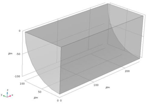
FIGURE 1. Basic schematic of straight tube generated using COMSOL.

The fluid was given a velocity of 0.004 m/s at the inlet boundary. The outlet boundary was set at p=0, referring to the inlet boundary. Fifty particles were injected from different positions at the inlet boundary to the outlet boundary. The details of the simulation model are listed in Table 1.

TABLE 1

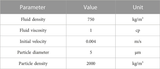
TABLE 1. Simulation inputs for the straight-tube model.

3.2 Fluid velocity profile and particle trajectory

The velocity profile and particle trajectory are illustrated in Figure 2. The flow velocity distribution across the tube follows the character of Poiseuille flow. With the only effect of the drag force, particles move along the flow streamline.

FIGURE 2

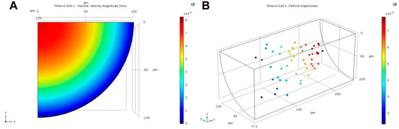
FIGURE 2. (A) Velocity profiles in the cross section and (B) particle trajectories in the straight-tube model. Color scale represents the magnitude of fluid and particle velocities.

Using the Hagen–Poiseuille Law, the fluid velocity at any given radius (r) inside the tube can be expressed as

$v_f\left(r\right)=v_{\max }\left[1-{\left(\frac{r}{R}\right)}^2\right],(10)$

where $v_{\mathit{max}}$ is the maximum fluid velocity inside the tube, and $R$ is the radius of the tube. In this case, $v_{\mathit{max}}$ is around 0.006 m/s, and $R$ is equal to 100 μm (0.0001m). Plugging them into Eq. 10, the velocity distribution inside the tube is

$v_f\left(r\right)=0.006\left[1-{\left(\frac{r}{1\times {10}^{-4}}\right)}^2\right].(11)$

3.3 Non-equilibrium parameter determination

The NE parameter ($\mathbf{1}-\frac{{\mathit{v}}_{\mathit{p}}}{{\mathit{v}}_{\mathit{f}}}$) was evaluated using COMSOL. Simulation results were matched with the harmonic oscillator equation using MATLAB^® to obtain the magnitude (A) and damping ratio (ζ) values. The P50 value on cumulative distribution functions (CDF) of A and ζ were recorded separately to represent the most likely value.

The NE parameter as a function of time for one of 50 particles is plotted in Figure 3A. At an early stage (when particle is just injected into the tube), there is velocity difference between the particle and fluid. In that time period, particle velocity is always less than fluid velocity. After a certain time period, the particle and fluid reach the same velocity, which can be described as an equilibrium state. The adapted harmonic oscillation equation (Eq. 9) was implemented to match simulation results using MATLAB. The curve-fitting result for a single particle is shown in Figure 3B.

FIGURE 3

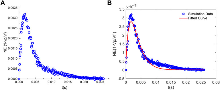
FIGURE 3. (A) NE parameter as a function of time solved using COMSOL, and (B) curve fitting for the NE effect of a single particle using MATLAB.

The same curve-fitting process was performed for all 50 particles. The histograms and cumulative distribution functions for two key factors of NE, A and ζ, are presented in Figure 4. The P50 values of A and ζ at their cumulative distribution functions are 0.025 and 0.977, respectively.

FIGURE 4

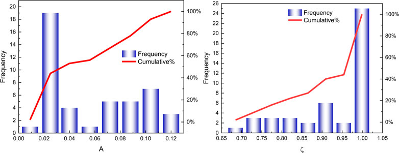
FIGURE 4. Histograms and CDFs of A and ζ values for the straight-tube model obtained from curve fitting.

3.4 Decouple particle equation from fluid equation

The P50 values of ${\mathit{\omega }}_{\mathbf{0}}$ and $\mathit{\phi }$ on their cumulative distribution functions were determined to be 305 and 100, respectively. Plugging the P50 values of all coefficients into Eq. 9, the following equation is obtained:

$1-\frac{v_p}{v_f}=0.025e^{-298t}\sin \left(66t+100\right),(12)$

Combining Eq. 11 with Eq. 12, the particle velocity for any given radius (r) and time (t) for the case of $\mu =1$ cp is determined to be

$v_p\left(r,t\right)=0.006\left[1-{\left(\frac{r}{1\times {10}^{-4}}\right)}^2\right]\left[1-0.025e^{-298t}\sin \left(66t+100\right)\right].(13)$

4 Converging–diverging tube model

4.1 Model setup and simulation results

In a real situation, the complex roughness geometries of fractures or porous media are often characterized by triangular, rectangular, trapezoidal, bell, sinusoidal, and random shapes (Dejam et al., 2018). In this work, for simplicity, a periodical converging–diverging-shaped tube is used to characterize porous media. The basic schematic of the converging–diverging-shaped tube model is demonstrated in Figure 5A. Two diverging-shaped tubes and one converging-shaped tube are connected with each other. Each tube has a maximum radius of 100 μm and a minimum radius of 50 μm, as well as a tube length of 250 μm. Fifty particles were injected at the same velocity with the initial fluid velocity from the inlet boundary to the outlet boundary. The details of the simulation are same as those of the straight-tube model except that the initial velocity is set to be 0.008 m/s. The fluid velocity profile and particle trajectory are illustrated in Figures 5B, C. Similar with the tube with uniform radius, the velocity distribution in the converging–diverging tube follows the character of Poiseuille flow. Fluid velocity magnitude is higher in the small-radius region compared to that in the big-radius region. The fluid velocity inside the tube was evaluated using COMSOL. For the cross sections with the radius of 100 μm and 50 μm, the maximum velocities are approximately 0.0045 m/s and 0.014 m/s, respectively.

FIGURE 5

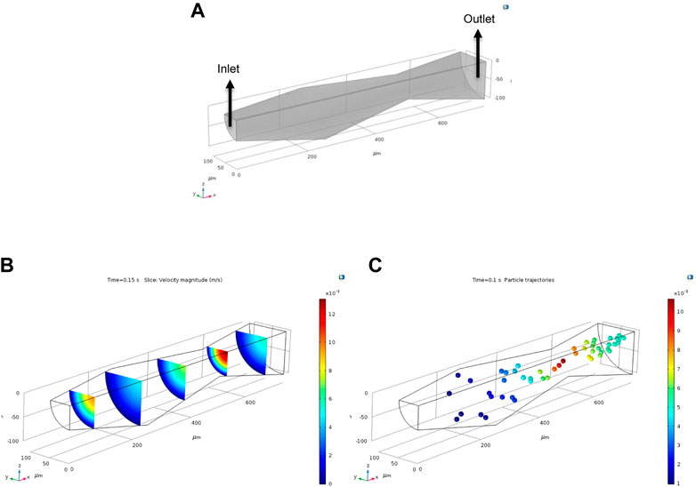
FIGURE 5. (A) Basic schematic of the converging–diverging tube generated using COMSOL. (B) Fluid velocity distribution and (C) particle trajectories inside the converging–diverging tube. Color scale represents the magnitude of fluid and particle velocities.

4.2 Fluid velocity profile

The velocity profile $\mathrm{v}\left(\mathrm{r},\mathrm{z}\right)$ in a tube whose cross-section area is gradually changing with the distance along the flow direction remains parabolic (Bahrami et al., 2008). The schematic velocity profile is shown in Figure 6.

FIGURE 6

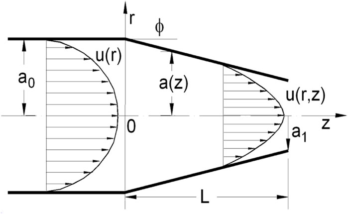
FIGURE 6. Schematic of varying the cross-section tube.

Therefore, the axial velocity needs to be described as

$u\left(r,z\right)=2u_m\left(z\right)\left[1-{\left(\frac{r}{a\left(z\right)}\right)}^2\right],(14)$

where $u_m\left(z\right)$ is the average velocity at the axial location z and $a\left(z\right)$ is the tube radius at the location z. By applying the conservation of mass, we obtain

$u_m\left(z\right)={\left[\frac{a_0}{a\left(z\right)}\right]}^2{u}_{m,0},(15)$

where $a_0$ is the tube radius at the initial point. Combining Eq. 14 and 15, the axial velocity equation is

$u\left(r,z\right)=2u_{m,0}{\left[\frac{a_0}{a\left(z\right)}\right]}^2\left[1-{\left(\frac{r}{a\left(z\right)}\right)}^2\right].(16)$

For a convergent-shaped tube,

$a\left(z\right)=R_{\min }+\frac{L-z}{L}\left(R_{\max }-R_{\min }\right),(17)$

where $R_{\mathit{min}}$, $R_{\mathit{max}}$, and $L$ are the minimum tube radius, maximum tube radius, and tube length, respectively. Similarly, for a divergent-shaped tube,

$a\left(z\right)=R_{\min }+\frac{z}{L}\left(R_{\max }-R_{\min }\right).(18)$

By combining Eq. 16 with Eq. 17, we get the generalized velocity equation in a converging tube, which is

$u\left(r,z\right)=2u_{m,0}{\left[\frac{a_0}{R_{\min }+\frac{L-z}{L}\left(R_{\max }-R_{\min }\right)}\right]}^2\left[1-{\left(\frac{r}{R_{\min }+\frac{L-z}{L}\left(R_{\max }-R_{\min }\right)}\right)}^2\right].(19)$

By combining Eq. 16 with Eq. 18, we get the generalized velocity equation in a diverging tube, which is

$u\left(r,z\right)=2u_{m,0}{\left[\frac{a_0}{R_{\min }+\frac{z}{L}\left(R_{\max }-R_{\min }\right)}\right]}^2\left[1-{\left(\frac{r}{R_{\min }+\frac{z}{L}\left(R_{\max }-R_{\min }\right)}\right)}^2\right].(20)$

Plugging $R_{\mathit{min}}=5\times {10}^{-5}\mathrm{m}$, $R_{\mathit{max}}=1\times {10}^{-4}\mathrm{m}$, $L=2.5\times {10}^{-4}\mathrm{m}$, and $2u_{m,0}$ =0.0045 m/s into Eq. 19, the fluid equation for any given radius (r) and axial length (z) inside the convergent is

$v_f\left(r,z\right)=4.5\times {10}^{-3}{\left[\frac{1\times {10}^{-4}}{1\times {10}^{-4}-\frac{z}{5}}\right]}^2\left[1-{\left(\frac{r}{1\times {10}^{-4}-\frac{z}{5}}\right)}^2\right].(21)$

Plugging $2u_{m,0}$ =0.014 m/s into Eq. 20, the fluid velocity equation for any given radius (r) and axial length (z) inside the divergent tube is

$v_f\left(r,z\right)=0.014{\left[\frac{5\times {10}^{-5}}{5\times {10}^{-5}+\frac{z}{5}}\right]}^2\left[1-{\left(\frac{r}{5\times {10}^{-5}+\frac{z}{5}}\right)}^2\right].(22)$

4.3 Non-equilibrium parameter determination

Following the same steps as the straight-tube model, the NE parameters were evaluated using COMSOL. Simulation results were matched with the harmonic oscillator equation to obtain the magnitude (A) and damping ratio (ζ) values. The P50 values on cumulative distribution functions (CDF) of A and ζ were recorded separately.

The NE parameter as a function of time is shown in Figure 7A According to the figure, the particle experiences three main stages depending on the flow path geometry. The flow geometry for the first stage is a divergent-shaped flow path. The NE parameter is less than zero, which means that particle velocity exceeds fluid velocity when the tube radius is getting bigger. At an early time, there is a big difference between the particle velocity and fluid velocity. At late time, particle velocity gets close to fluid velocity, indicating they are close to the equilibrium state. After the first stage, the flow path geometry switches to a convergent shape. The NE parameter is larger than zero. It implies that particle velocity is always less than fluid velocity. In contrary to system behavior in the divergent flow path, the particle and fluid velocity will never getting close to each other, which indicates that the non-equilibrium will always happen. The reason for the NE parameter drops at late time is because the flow path geometry transits from converting to a diverging pattern.

FIGURE 7

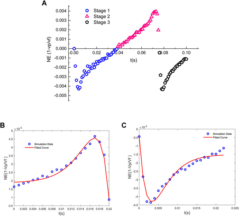
FIGURE 7. (A) NE parameters as a function of time in the converging–diverging tube solved using COMSOL, and the curve fitting of NE for single particle injection for (B) stage 2, and (C) stages 1 and 3 using MATLAB.

The harmonic oscillation equation was implemented to match simulation results for different stages separately. The initial time for all three stages was normalized to zero for curve fitting. The curve fitting result for a single particle in stage 2 is shown in Figure 7B. The A and ζ values were determined to be $2.4\times {10}^{-5}$ and -0.978. In frictional vibration, negative damping causes system instability (Chen, 2014). In this situation, it indicates that the NE parameter increases as a function of time. Since particle flowed in the converging tube, it can be concluded that the negative ζ value implies particle to move in convergent flow path geometry. Stage 1 and stage 3 had same particle-fluid behavior, and the fitting curve is shown in Figure 7C. The A and ζ values were determined to be 0.026 and 0.94. In this case, ζ equals to a positive number. It means that the NE parameter decreases over time. Since particle flowed in the diverging flow path, it can be concluded that the positive ζ value is an indication of particle moving in divergent flow pattern.

After matching all 50 particles’ data, the histograms and cumulative distribution function for A and ζ in divergent and convergent flow patterns were obtained separately. The P50 values of A and ζ for the convergent flow pattern are determined to be $1.9\times {10}^{-5}$ and -0.894, respectively. As for divergent flow path geometry, P50 values for A and ζ are 0.015 and 0.926, respectively. The result complies with the single particle case where ζ is negative when the flow pattern is convergent, whereas ζ is positive when the flow pattern is divergent shape. Moreover, the result indicates that the A value for the convergent flow pattern is smaller than that of the divergent flow pattern.

4.4 Decouple particle equation from the fluid equation

The particle transport equation is obtained by combining the fluid equation with the NE equation. All coefficients in the harmonic oscillation equation that are used to describe NE were obtained from P50 values on their cumulative distribution functions. The P50 values of A, ζ, ${\mathit{\omega }}_{\mathbf{0}}$, and $\mathit{\phi }$ for convergent flow path geometry are 1.9×10^–5, -0.894, 421, and 100, respectively.

Plugging P50 values of those coefficients into Eq. 9, the NE equation for the convergent flow pattern is

$1-\frac{v_p}{v_f}=1.9\times {10}^{-5}{e}^{376t}\sin \left(189t+100\right).(23)$

By combining Eq. 21 with Eq. 23, we get the particle velocity equation for any given radius (r), axial location (z), and time (t) in the convergent tube, which is

$\begin{array}{l}{v}_p\left(r,z,t\right)=4.5\times {10}^{-3}{\left[\frac{1\times {10}^{-4}}{1\times {10}^{-4}-\frac{z}{5}}\right]}^2\left[1-{\left(\frac{r}{1\times {10}^{-4}-\frac{z}{5}}\right)}^2\right]\left[1-1.9\times {10}^{-5}{e}^{376t}\sin \left(189t+100\right)\right]\\ t\in \left[\mathrm{0,0.025}\right],z\in \left[\mathrm{0,2.5}\times {10}^{-4}\right].\end{array}(24)$

Coefficients (A, ζ, ${\mathrm{\omega }}_0$, and $\mathrm{\phi }$) for divergent flow path geometry are 0.015, 0.926, 237, and 100.

Plugging P50 values of those coefficients into Eq. 9, the NE equation for the divergent flow pattern is obtained as

$1-\frac{v_p}{v_f}=0.015e^{-220t}\sin \left(90t+100\right),(25)$

By combining Eq. 22 with Eq. 25, the particle velocity equation for any given radius (r), axial location (z), and time (t) in the convergent tube is determined to be

$\begin{array}{l}{v}_p\left(r,z,t\right)=0.014{\left[\frac{5\times {10}^{-5}}{5\times {10}^{-5}+\frac{z}{5}}\right]}^2\left[1-{\left(\frac{r}{5\times {10}^{-5}+\frac{z}{5}}\right)}^2\right]\left[1-0.015e^{-220t}\sin \left(90t+100\right)\right]\\ t\in \left[\mathrm{0,0.025}\right],z\in \left[\mathrm{0,2.5}\times {10}^{-4}\right].\end{array}(26)$

In order to validate the accuracy of the particle velocity equation that decoupled from the fluid equation, the predicted particle velocities with different initial locations for convergent and divergent flow path geometries from the analytical particle velocity equation are compared with the simulation results solved using COMSOL Multiphysics^®. The results are shown in Figure 8. It is shown in the figure that there are decent matches between the analytical result and simulation result, which proves the accuracy of the model.

FIGURE 8

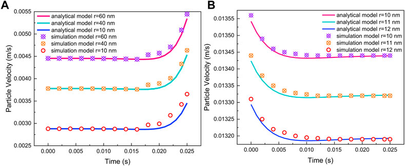
FIGURE 8. Comparison of particle velocities solved by the analytical model and simulation model for (A) convergent and (B) divergent flow path geometries.

5 Non-equilibrium effects in the actual pore network

5.1 Model setup and simulation results

The model geometry that we used is a SEM image of a real pore network from the COMSOL application library. The binary image and imported geometry are shown in Figure 9A. The size of the image is 640 μm by 320 μm. The black region represents the pore space. The white region represents the rock grain. The single particle was injected from the inlet (right side) to outlet (left side) boundary in the same velocity as the fluid velocity. The particle and fluid properties are set to be the same as those of the straight-tube model. The fluid velocity distribution and single particle trajectory inside the pore structure are demonstrated in Figures 9B, C.

FIGURE 9

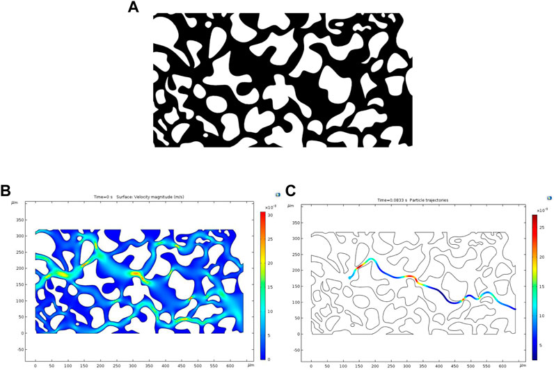
FIGURE 9. (A) SEM images of the pore structure in a binary format. (B) Fluid velocity field and (C) particle trajectory in the pore network solved using COMSOL. Color scales represent the magnitude of fluid and particle velocities.

5.2 Pore size distribution from SEM images

The pore size distribution is determined using the MATLAB code designed by Rabbani et al. (2014). It is based on the watershed segmentation algorithm, which can detect and separate pores by cutting the image on the watershed ridge line. Assuming that each segment is a circle, the pore radius can be determined. The cut structure and pore size distribution are shown in Figure 10.

FIGURE 10

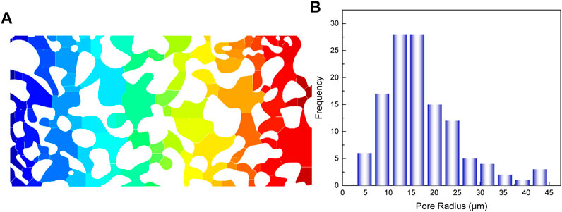
FIGURE 10. (A) Separation of pores based on the watershed segmentation algorithm, and (B) the pore size distribution of the SEM pore structure.

5.3 Non-equilibrium parameter determination

The NE effect for the single particle was evaluated using COMSOL. The NE as a function of time for a single particle injection is plotted in Figure 11A. Due to the complexity of the pore structure, the trends of NE variation over time are not identical. As discussed earlier, NE larger than zero indicates that particles move through the converging flow pattern, whereas NE less than zero implies that particles move in the diverging flow pattern. In addition, different-shaped pores are supposed to have different oscillation behaviors, which manifest as distinct curve shapes in the figure. Therefore, based on the flow pattern criteria and the shape of the NE curve, the NE curve can be divided into several stages. For example, from t=0 to t=0.01s, the NE is above zero, which is an indication of converging flow path geometry. Meanwhile, there are two distinct curve shapes, which means that the particle moves in two different pores.

FIGURE 11

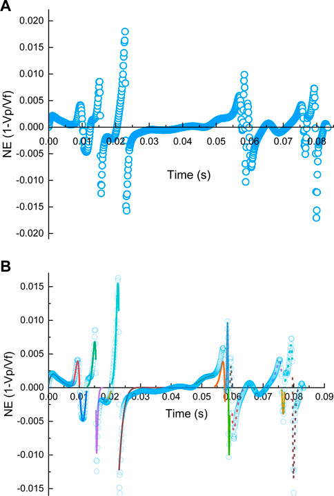
FIGURE 11. (A) NE as a function of time for a single particle injection in the pore structure. (B) Fitted NE curves for 20 stages. Each color represents one stage. Blue circles are the original data.

After detecting the flow path and the curve shape, 20 stages were identified. Again, the adapted harmonic oscillation equation was implemented to match the data for each stage. The initial time for each stage was normalized to zero for curve fitting. The oscillator amplitudes and damping ratios were obtained and are demonstrated in Table 2. The results present that in the converging flow pattern, ζ values are less than zero, which is consistent with the result obtained in the previous model. It means that the particle velocity is always less than the fluid velocity, and they can never achieve equilibrium with each other. In the diverging flow pattern, the result shows that ζ values are greater than zero, which is also consistent with the previous observation. As discussed earlier, particle velocity is greater than fluid velocity in the diverging flow path. Using all coefficients (A, ζ, ${\mathrm{\omega }}_0$, and $\mathrm{\phi }$) obtained from the curve fitting, the matched NE curve for all stages can be obtained, and they are shown in Figure 11B. The fitted curves have good matches with the original NE curve, which are evaluated in simulation.

TABLE 2

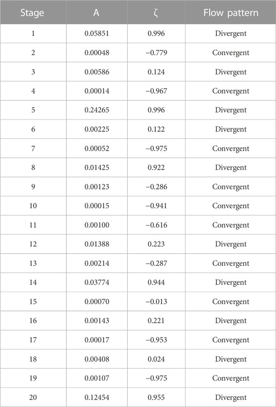
TABLE 2. A and ζ values for 20 stages obtained from curve fitting. Flow patterns for each stage are indicated.

5.4 Equivalent tube radius determination for the pore structure

In order to have a better characterization of particle transport behavior in porous media, the motions of multiple particles in different size of pores need to be investigated. Simulations were performed for different numbers of particle injections. The simulation details are kept same as those of the straight-tube model.

The simulation was performed on 5–20 particle injections (Jin, 2018). There are some pore spaces that particles can never reach with only the effect of drag force. Moreover, it was observed that some particles share same paths inside the pore structure. The more particles are injected, the more repeated flow paths are observed. Therefore, some tube radii will be calculated more than once finally yielding an over-estimation of equivalent pore number. Therefore, in this case, five particles’ trajectories have covered almost all possible flow paths that particles can reach. It provides a better characterization of the pore network, and the corresponding tube radius distribution is considered the actual pore spaces that particles move through in this pore network.

In order to determine the radius distribution of pores that particles move through, the MATLAB code was designed to identify different stages in which particles move through different sizes of pores, and then the proposed NE equation was applied to match the results for all stages to obtain the A values.

The rationale for defining an equivalent radius is that since each stage has its corresponding A value in multiple particles’ injection simulation, it is hypothesized that there is an equivalent tube radius that can give the same A value for each stage. In order to determine the equivalent pore radii for all stages, another converging–diverging model simulation, which has been discussed in section 4, was performed. According to the pore size distribution of the pore structure, the minimum and maximum pore radii are 4.81 μm and 43 μm, respectively. The converging–diverging models were set up with a fixed minimum tube radius of 5 μm, and the variable maximum tube radius ranged from 10 μm to 45 μm. The length of each tube was set at 50 μm.

The proposed NE equation was applied again to match the simulation results for the convergent and divergent flow pattern separately to obtain A values in different flow patterns. The relationships between the maximum radius and A value for convergent and divergent flow patterns are shown in Figure 12. The results indicate that there are approximately linear relationships between the tube radius and A value for different flow patterns.

FIGURE 12

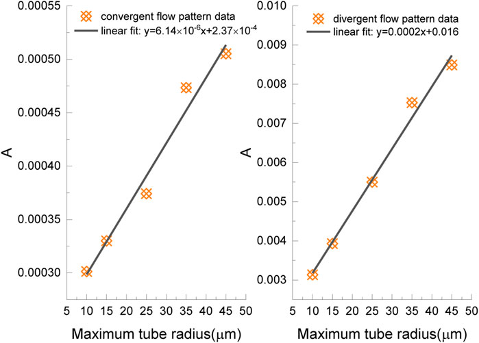
FIGURE 12. Corresponding A values for different maximum radii in the convergent flow pattern and divergent flow pattern.

Using the trend line equations, the maximum radius for each A value can be determined. The average value of maximum and minimum tube radii was approximated to be the equivalent tube radius of the corresponding stage. For the convergent flow pattern, the equivalent tube radius ($r_e$) is estimated to be

$r_e=\frac{R_{\max }+R_{\min }}{2}=79375.5A-16.(27)$

For the divergent flow pattern, the equivalent tube radius ($r_e$) is estimated to be

$r_e=\frac{R_{\max }+R_{\min }}{2}=3116.7A-2.3.(28)$

The estimated equivalent pore radius distribution for paths where five particles move through is shown in Figure 13.

FIGURE 13

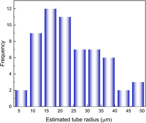
FIGURE 13. Histograms for the estimated tube radius for the five-particle injection scheme.

6 Conclusion

In this study, the NE effect in the particulate flow system was investigated by developing particle transport models in the straight tube, periodic converging–diverging-shaped tube, and actual pore structure. This study was hypothesizing whether the linear theory of stability can explain NE evolution in particulate systems through the general form of the harmonic oscillation equation. Particle velocity equations for convergent and divergent flow patterns are decoupled from fluid equations by incorporating the proposed NE equation. In this work, only particle–fluid interaction is taken into consideration; the drag force is the dominant factor, and the carrier fluid is a single-phase fluid. The main conclusions are drawn as follows:

1) The time variation of the NE effect complies with the theory of stability. The harmonic oscillation equation can be used to characterize the NE effect in the particulate flow system.

2) Two key parameters of the oscillator equation are amplitude (A) and damping ratio (ζ). The former represents the magnitude of NE and the latter is an indication of flow path geometry.

3) In divergent flow path geometry, the ζ value is between 0 and 1. The NE effect decreases as a function of time. The ζ value is between 0 and -1 in convergent flow path geometry where the NE effect increases as a function of time implying that the particle velocity always remains less than the fluid velocity; hence, the system will never achieve an equilibrium state.

4) The derived particle equation offers a quick estimation of particle velocity for a given time and the location of porous media.

5) The flow simulations of the SEM image present consistent results with diverging and converging flow results. By conducting different numbers of particle injection schemes, it is found that five-particle injection offers a better estimation of actual pores that particles move through. The corresponding equivalent tube radii of complex pore geometries are obtained.

Data availability statement

The original contributions presented in the study are included in the article/Supplementary Material; further inquiries can be directed to the corresponding author.

Author contributions

YJ: main idea proposing, numerical simulation, data analysis, and draft writing. ZZ: model validation, data analysis, and draft reviewing. RM: main idea and method proposing. All authors contributed to the article and approved the submitted version.

Acknowledgments

The authors acknowledge the donors of the American Chemical Society Petroleum Research Fund for supporting (or partial support) this research (PRF 56929-DN19).

Conflict of interest

Authors YJ and ZZ were employed by CNOOC Research Institute Co., Ltd., Beijing, China.

The remaining author declares that the research was conducted in the absence of any commercial or financial relationships that could be construed as a potential conflict of interest.

Publisher’s note

All claims expressed in this article are solely those of the authors and do not necessarily represent those of their affiliated organizations, or those of the publisher, the editors, and the reviewers. Any product that may be evaluated in this article, or claim that may be made by its manufacturer, is not guaranteed or endorsed by the publisher.

Abbreviations

$NE$, non-equilibrium; $\rho$, fluid density; $\mu$, fluid viscosity; F, forces acting on fluid; $F_D$, drag force; $m_P$, mass of the particle; ${\tau }_P$, relaxation time; $v_p$, particle velocity; $v_f$, local fluid velocity; $A$, oscillation amplitude; ζ, damping ratio; ${\omega }_0$, parameter in harmonic oscillation equation; $\phi$, parameter in harmonic oscillation equation; r, tube radius; $v_{\mathit{max}}$, maximum fluid velocity inside the tube; $R$, radius of the tube; t, time; z, axial location in the tube; $u_m\left(z\right)$, average velocity at the axial location z; $a\left(z\right)$, tube radius at location z; $R_{\mathit{min}}$, minimum tube radius; $R_{\mathit{max}}$, maximum tube radius; $L$, tube length; $r_e$, equivalent tube radius.

References

Amaratunga, M., Rabenjafimanantsoa, H. A., and Time, R. W. (2021). Influence of low-frequency oscillatory motion on particle settling in Newtonian and shear-thinning non-Newtonian fluids. J. Petroleum Sci. Eng. 196, 107786. doi:10.1016/j.petrol.2020.107786

CrossRef Full Text | Google Scholar

Awad, A. M., Hussein, I. A., Nasser, M. S., Karami, H., and Ahmed, R. (2021). CFD modeling of particle settling in drilling fluids: Impact of fluid rheology and particle characteristics. J. Petroleum Sci. Eng. 199, 108326. doi:10.1016/j.petrol.2020.108326

CrossRef Full Text | Google Scholar

Bahrami, M., Akbari, M., and Sinton, D. (2008). “Laminar fully developed flow in periodically converging-diverging microtubes,” in International conference on nanochannels, microchannels, and minichannels, 48345, 181–188.

CrossRef Full Text | Google Scholar

Bedrikovetsky, P., Siqueira, F. D., Furtado, C. A., and Souza, A. L. S. (2011). Modified particle detachment model for colloidal transport in porous media. Transp. porous media 86 (2), 353–383. doi:10.1007/s11242-010-9626-4

CrossRef Full Text | Google Scholar

Chen, G. S. (2014). Handbook of friction-vibration interactions. Elsevier.

Google Scholar

Davudov, D., Moghanloo, R. G., and Flom, J. (2018). Scaling analysis and its implication for asphaltene deposition in a Wellbore. SPE J. 23 (02), 274–285. doi:10.2118/187950-pa

CrossRef Full Text | Google Scholar

Dejam, M., Hassanzadeh, H., and Chen, Z. (2018). Shear dispersion in a rough-walled fracture. SPE J. 23 (05), 1669–1688. doi:10.2118/189994-pa

CrossRef Full Text | Google Scholar

Fan, M., McClure, J., Han, Y., Li, Z., and Chen, C. (2018). Interaction between proppant compaction and single-/multiphase flows in a hydraulic fracture. SPE J. 23 (04), 1290–1303. doi:10.2118/189985-pa

CrossRef Full Text | Google Scholar

Hu, Z., Azmi, S. M., Raza, G., Glover, P. W., and Wen, D. (2016). Nanoparticle-assisted water-flooding in Berea sandstones. Energy & fuels 30 (4), 2791–2804. doi:10.1021/acs.energyfuels.6b00051

CrossRef Full Text | Google Scholar

Jin, Y. (2018). Modeling of non-equilibrium effects in particulate flow through porous media.

Google Scholar

Kong, X., McAndrew, J., and Cisternas, P. (2016). “CFD study of using foam fracturing fluid for proppant transport in hydraulic fractures,” in Proceeding of the Abu Dhabi International Petroleum Exhibition & Conference, Abu Dhabi, UAE, November 2016 (OnePetro).

CrossRef Full Text | Google Scholar

Marquez, M., Williams, W., Knobles, M., Bedrikovetsky, P., and You, Z. (2014). Fines migration in fractured wells: Integrating modeling with field and laboratory data. SPE Prod. Operations 29 (04), 309–322. doi:10.2118/165108-pa

CrossRef Full Text | Google Scholar

Rabbani, A., Jamshidi, S., and Salehi, S. (2014). An automated simple algorithm for realistic pore network extraction from micro-tomography images. J. Petroleum Sci. Eng. 123, 164–171. doi:10.1016/j.petrol.2014.08.020

CrossRef Full Text | Google Scholar

Roy, P., Du Frane, W. L., and Walsh, S. D. (2015). “Proppant transport at the fracture scale: Simulation and experiment,” in Proceeding of the 49th US Rock Mechanics/Geomechanics Symposium, San Francisco, June 2015 (OnePetro).

Google Scholar

Song, S., and Park, S. (2019). “Numerical simulations of sediment transport and scour around monopile using CFD and DEM coupling,” in Proceeding of the 29th International Ocean and Polar Engineering Conference, Honolulu, USA, June 2019 (OnePetro).

Google Scholar

Sun, X., Zhang, Y., Chen, G., and Gai, Z. (2017). Application of nanoparticles in enhanced oil recovery: A critical review of recent progress. Energies 10 (3), 345. doi:10.3390/en10030345

CrossRef Full Text | Google Scholar

Wang, Y., Tao, Y., Ma, Z., and Zhou, L. (2019). “Development of particle-scale CFD-DEM models and application to hydraulic analysis of marine sand,” in Proceeding of the 29th International Ocean and Polar Engineering Conference, Honolulu, Hawaii, USA, June 2019 (OnePetro).

Google Scholar

Yu, W., and Sepehrnoori, K. (2013). “Simulation of proppant distribution effect on well performance in shale gas reservoirs,” in Proceeding of the SPE Unconventional Resources Conference Canada, Calgary, Alberta, Canada, November 2013 (OnePetro).

CrossRef Full Text | Google Scholar

Yuan, B., Moghanloo, R. G., and Zheng, D. (2016). Analytical evaluation of nanoparticle application to mitigate fines migration in porous media. Spe J. 21 (06), 2317–2332. doi:10.2118/174192-pa

CrossRef Full Text | Google Scholar

Yuan, H., and Shapiro, A. A. (2010). Modeling non-Fickian transport and hyperexponential deposition for deep bed filtration. Chem. Eng. J. 162 (3), 974–988. doi:10.1016/j.cej.2010.07.003

CrossRef Full Text | Google Scholar