Coupling fraction model to interpret the motion of non-fully coupled strike-slip faults

Despite coupling fractions being extensively used in the interseismic period, the coexistence of locking and creeping mechanisms and the correlation between the coupling fraction and locking depth remain poorly understood because of the lack of a physical model. To overcome these limitations, in this study, we propose a coupling fraction model for interpreting the motion of non-fully coupled strike-slip faults based on the classic two-dimensional strike-slip fault model and the superposition principle. The model was constructed using numerous tiny, alternating creeping and locking segments. The deformation produced by the model is the same as that of the classic two-dimensional strike-slip fault, except for the scale factor. The model and definition of the coupling fraction can be perfectly integrated. Based on the model, we put forward a varying decoupled fraction with depth model, which considers the depth-dependent coupling fraction. The two models provide deep insights into the deformation characteristics of quasi-arctangent curves produced by non-fully coupled strike-slip faults and the local and macroscopic characteristics of fault locking in the interseismic period.

1 Introduction

Dislocation theory, which interprets fault-motion-based deformation on the surface, has become an important physical model since the elastic rebound theory was put forward (Reid 1910; Chinnery, 1963; Okada 1985, 1992; Matsu’ura et al., 1986; Sun and Okubo, 1993, 1998; Wang et al., 2003; Steketee, 1958; Pan, 2019; Dong et al., 2021). The simplest representation of dislocation along an infinitely deep and long strike-slip fault is shown in Figure 1A. Savage and Burford (1973) reported the equation for the velocity of the model (SB73 model)—represented by a straight and vertical fault in an elastic half-space, in which uniform slip equal to the free slip rate occurs on the fault below the depth, above which the fault is fully coupled—as follows:

$\mathit{v}=\frac{\mathit{s}}{\mathit{\pi }}{\mathit{tan}}^{-\mathbf{1}}\left(\frac{\mathit{x}}{\mathit{d}}\right),(1)$

where x is the distance from the fault and d is the locking depth, which means that the fault above d is fully coupled/locked, whereas the fault below d is fully creeping. The parameter s is the free slip rate below d (Figures 1A, B). The curve produced by the SB73 model is an arctangent function (Figure 1B). Furthermore, the coupling fraction (or fault locking), which quantifies the slip deficit on the patch of a seismogenic zone relevant to the free creep below the patches, was introduced to describe the locking degrees from the shallow to the deep parts of the fault (McCaffrey et al., 2000; McCaffrey, 2002; McCaffrey, 2005; Scholz, 2007). The coupling fraction $\delta$ is defined as follows:

$\mathit{\delta }=\mathbf{1}-\frac{{\mathit{S}}_{\mathit{c}}}{\mathit{S}},(2)$

where s is the free slip rate and s_c represents the creeping part of the non-fully coupled fault. Based on negative dislocation theory (Matsu’ura et al., 1986), the locking degrees of faults can be obtained by the inversion of surface deformation on each patch and used to estimate the seismic risk of the fault (Jiang et al., 2015; Zhao et al., 2020; Li et al., 2021a; Li et al., 2021b; Jian et al., 2022; Li et al., 2022).

FIGURE 1

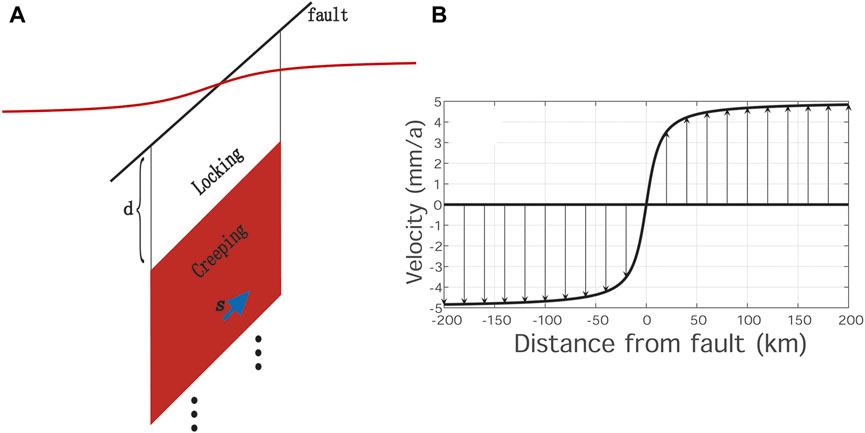
FIGURE 1. (A) Classic 2D strike-slip fault model and (B) produced surface deformation (redrawn according to Savage and Burford, 1973). A dextral strike-slip fault with a slip rate of 10 mm/a and a locking depth of 10 km was used as an example.

Although the coupling fraction has been widely used in the interseismic period, questions remain regarding the coexistence of locking and creeping mechanisms, and the correlation between the coupling fraction and locking depth, because of the lack of a physical model. Why can the slip and lock happen at the same time during fault motion, and what is the physical meaning of the coupling fraction? In this study, an appropriate two-dimensional coupling fraction (CF) fault model is proposed for interpreting the motion of non-fully coupled strike-slip faults based on the SB73 model and the superposition principle. In addition, a varying decoupled fraction with depth (VDFD) model is established, based on the CF model, to expand the model’s applications. Two models interpreting the motion of the non-fully coupled strike-slip fault can help us to understand why and how the faults can be creeping and locking at the same time.

2 Model with non-fully coupled strike-slip fault

In our discussion, a fault segment that is fully coupled or locked is called a locking segment, and a fault segment that is fully creeping or slipping is called a creeping segment. The length of the fault segment is called the segment length, and the function $\mathrm{C}f\left(d,L\right)$ represents the surface slip distribution by the fault segment, for which the vertical distance from the upper edge of the fault to the surface is d and the segment length is L (Figure 2A). Based on the superposition principle and the SB73 model, the CF and VDFD models are proposed in this study.

FIGURE 2

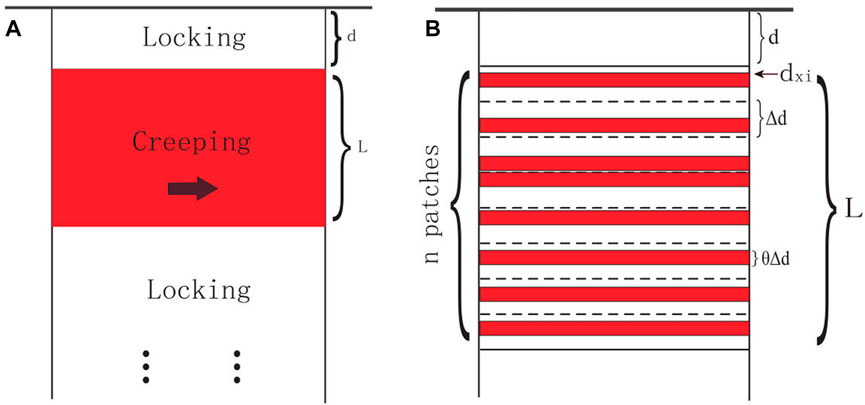
FIGURE 2. Red and white patches represent creeping and locking segments, respectively. (A) Model of the strike-slip fault with a finite locking segment length. Surface deformation is $\frac{s}{\pi }\left({\mathit{tan}}^{-1}\frac{x}{d}-{\mathit{tan}}^{-1}\frac{x}{d+L}\right)$. (B) Schematic of the coupling fraction fault (CF) model construction.

2.1 Model of the strike-slip fault with a finite locking segment length

The model for the slip distribution of the strike-slip fault with a finite locking segment length can be expressed as follows (Figure 2A):

$\mathrm{C}f\left(d,L\right)=\frac{\mathit{s}}{\mathit{\pi }}\left({\mathit{tan}}^{-\mathbf{1}}\frac{\mathit{x}}{\mathit{d}}-{\mathit{tan}}^{-\mathbf{1}}\frac{\mathit{x}}{\mathit{d}+\mathit{L}}\right).(3)$

It can be constructed based on the superposition principle and the SB73 model, or directly derived from screw dislocation (Savage and Burford, 1973; Savage, 1990; Segall, 2010).

2.2 Construction of the CF model

Based on the model mentioned previously, the locking segment is laid from the surface to depth d and the fault segment below d, where the segment length L is divided into n patches and the segment length of each patch is $∆d$, with $∆d=\frac{n}{L}$. The creeping segments with segment lengths of $\theta \bullet d$ are then laid on the random position of each patch (Figure 2B). Therefore, the total surface deformation $\mathrm{C}f\left(d,L\right)$ is the sum of the surface deformation of each creeping segment based on the superposition principle:

$\mathbf{C}\mathit{f}\left(\mathit{d},\mathit{L}\right)={\displaystyle \sum }_{\mathit{i}=\mathbf{1}}^{\mathit{n}}\frac{\mathit{s}}{\mathit{\pi }}\left[{\mathit{tan}}^{-\mathbf{1}}\left(\frac{\mathit{x}}{{\mathit{d}}_{{\mathit{x}}_{\mathit{i}}}}\right)-{\mathit{tan}}^{-\mathbf{1}}\left(\frac{\mathit{x}}{{\mathit{d}}_{{\mathit{x}}_{\mathit{i}}}+\mathit{\theta }\frac{\mathit{n}}{\mathit{L}}}\right)\right],(4)$

where $d\ge 0$, $0<\theta \le 1$, $i=\mathrm{1,2},\cdots n$, and $d_{x_i}$ represents each of the upper edges of the creeping segment, which is a random value in the interval $\left[d+\left(i-1\right)∆d,d+i∆d-\theta ∆d\right]$, $i=\mathrm{1,2},\cdots n$. When n is very large, $\mathrm{C}f\left(d,L\right)$ approaches a result which is $\theta \bullet \frac{s}{\pi }\left({\mathit{tan}}^{-1}\frac{x}{d}-{\mathit{tan}}^{-1}\frac{x}{d+L}\right)$ (Figure 3). Therefore, the CF model $\mathbf{C}\mathit{f}\left(\mathit{d},\mathit{L},\mathit{\theta }\right)$ is expressed as follows:

$\mathbf{C}\mathit{f}\left(\mathit{d},\mathit{L},\mathit{\theta }\right)=\underset{\mathit{n}\to \mathit{\infty }}{\mathbf{lim}}{\displaystyle \sum }_{\mathit{i}=\mathbf{1}}^{\mathit{n}}\frac{\mathit{s}}{\mathit{\pi }}\left[{\mathit{tan}}^{-\mathbf{1}}\left(\frac{\mathit{x}}{{\mathit{d}}_{{\mathit{x}}_{\mathit{i}}}}\right)-{\mathit{tan}}^{-\mathbf{1}}\left(\frac{\mathit{x}}{{\mathit{d}}_{{\mathit{x}}_{\mathit{i}}}+\mathit{\theta }∆\mathit{d}}\right)\right].(5)$

FIGURE 3

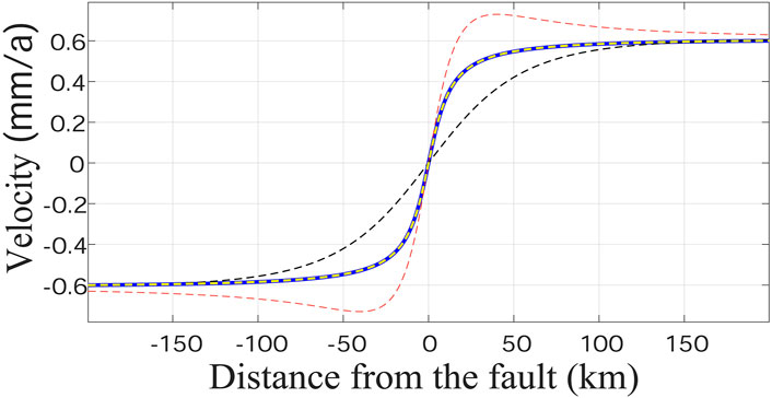
FIGURE 3. Curves obtained from the numerical simulation of $\mathrm{C}f\left(d,L\right)$. $\theta$ value is 0.4, d is 10 km, L is 10,000 km (without considering the actual situation, only for the validation of the model), s is $\pi$ mm/a, and the thick blue line is $\theta \bullet \frac{s}{\pi }\left({\mathit{tan}}^{-1}\frac{x}{d}-{\mathit{tan}}^{-1}\frac{x}{d+L}\right)$. Red and black dashed lines are the curves of $\mathrm{C}f\left(d,L\right)$ when n = 100. The curves are over- or underloaded because of the random positions of creeping segments in each patch; yellow dashed line (n = 10,000) and blue line overlap.

This model represents the surface deformation caused by numerous tiny creeping segments that are separated by locking segments. As shown in Figure 2B, the creeping part of the fault segment with segment length L is discontinuous in depth when n is very large.

We applied the Lagrange mean value theorem, $\forall i$, as follows:

${\mathit{tan}}^{-\mathbf{1}}\left(\frac{\mathit{x}}{{\mathit{d}}_{{\mathit{x}}_{\mathit{i}}}}\right)-{\mathit{tan}}^{-\mathbf{1}}\left(\frac{\mathit{x}}{{\mathit{d}}_{{\mathit{x}}_{\mathit{i}}}+\mathit{\theta }∆\mathit{d}}\right)=-\frac{\mathit{\theta }\mathit{L}}{\mathit{n}}{\bullet \left.\frac{\mathit{d}\left({\mathit{tan}}^{-\mathbf{1}}\frac{\mathit{x}}{\mathit{\zeta }}\right)}{\mathit{d}\mathit{\zeta }}\right|}_{\mathit{\zeta }={\mathit{\zeta }}_{\mathit{i}}},$

where ${\zeta }_i\in \left[d_{x_i},d_{x_i}+\frac{n}{L}\right]$

$\therefore \mathit{C}\mathit{f}\left(\mathit{d},\mathit{L},\mathit{\theta }\right)=-\frac{\mathit{\theta }\mathit{s}}{\mathit{\pi }}\underset{\mathit{n}\to \infty }{\mathbf{lim}}{\displaystyle \sum }_{\mathit{i}=\mathbf{1}}^{\mathit{n}}\frac{\mathit{L}}{\mathit{n}}{\bullet \left.\frac{\mathit{d}\left({\mathit{tan}}^{-\mathbf{1}}\frac{\mathit{x}}{\mathit{\zeta }}\right)}{\mathit{d}\mathit{\zeta }}\right|}_{\mathit{\zeta }={\mathit{\zeta }}_{\mathit{i}}}$

$=-\frac{\mathit{\theta }\mathit{s}}{\mathit{\pi }}{\int }_{\mathbf{d}}^{\mathit{d}+\mathit{L}}\frac{\mathit{d}\left({\mathit{tan}}^{-\mathbf{1}}\frac{\mathit{x}}{\mathit{\zeta }}\right)}{\mathit{d}\mathit{\zeta }}\mathit{d}\mathit{\zeta }=\frac{\mathit{\theta }\mathit{s}}{\mathit{\pi }}\left({\mathit{tan}}^{-\mathbf{1}}\frac{\mathit{x}}{\mathit{d}}-{\mathit{tan}}^{-\mathbf{1}}\frac{\mathit{x}}{\mathit{d}+\mathit{L}}\right),(6)$

where $\theta$ is called the “decoupled fraction” or “fault creeping” in Formula 6 (strict proof is provided in the Supplementary Material).

The CF model is derived from the superposition principle and the SB73 model, which ensure the correctness of the model in theory. The construction of the CF model shows that numerous, tiny creeping segments alternate with the locking segments. The results of the CF model illustrate that the sum of the deformation by these creeping segments is the same as the deformation by the large creeping segment in Figure 2A, except for the scale factor $\theta$. Figure 3 shows the results of the comparison between $Cf\left(d,L,\theta \right)$ and $\mathrm{C}f\left(d,L\right)$. When n is not large enough, which also means that the creeping segments are not small enough, the curves are over- or underloaded because of the random positions of creeping segments in each patch. When n increases, $Cf\left(d,L\right)$ and $Cf\left(d,L,\theta \right)$ quickly coincide.

2.3 Correlation between $\mathit{\theta }$ and $\mathit{\delta }$

The $\theta$ parameter in the CF model is derived from superposition and the SB73 model, whereas $\delta$ is defined by the equation (McCaffrey, 2002). In this study, the correlation between $\theta$ and $\delta$ is discussed. First, $Cf\left(0,L,\theta \right)$ and $Cf\left(d,\infty ,\theta \right)$ must be derived using Formula 6 (Figure 4):

$\mathit{C}\mathit{f}\left(\mathbf{0},\mathit{L},\mathit{\theta }\right)=\underset{\mathit{d}\to \mathbf{0}}{\mathbf{lim}}\mathit{C}\mathit{f}\left(\mathit{d},\mathit{L},\mathit{\theta }\right)=\frac{\mathit{\theta }\mathit{s}}{\mathit{\pi }}\bullet \left(\frac{\mathit{\pi }}{\mathbf{2}}\bullet \mathit{s}\mathit{g}\mathit{n}\left(\mathit{x}\right)-{\mathit{tan}}^{-\mathbf{1}}\frac{\mathit{x}}{\mathit{L}}\right)=\frac{\mathit{\theta }\mathit{s}}{\mathit{\pi }}\bullet {\mathit{tan}}^{-\mathbf{1}}\frac{\mathit{L}}{\mathit{x}},(7)$

$\mathit{C}\mathit{f}\left(\mathit{d},\mathit{\infty },\mathit{\theta }\right)=\underset{\mathit{L}\to \mathit{\infty }}{\mathbf{lim}}\mathit{C}\mathit{f}\left(\mathit{d},\mathit{L},\mathit{\theta }\right)=\frac{\mathit{\theta }\mathit{s}}{\mathit{\pi }}\bullet {\mathit{tan}}^{-\mathbf{1}}\frac{\mathit{x}}{\mathit{d}},(8)$

where $sgn\left(x\right)$ is the signum function. Based on the negative dislocation (Matsu’ura et al., 1986), the slip distribution of the strike-slip fault with the coupling fraction $\delta$ can be expressed as follows:

$\frac{\mathit{s}}{\mathbf{2}}\mathit{s}\mathit{g}\mathit{n}\left(\mathit{x}\right)-\frac{\mathit{\delta }\mathit{s}}{\mathit{\pi }}{\mathit{tan}}^{-\mathbf{1}}\left(\frac{\mathit{d}}{\mathit{x}}\right),$

where $\frac{s}{2}sgn\left(x\right)$ is the free slip rate and $\frac{\delta s}{\pi }{\mathit{tan}}^{-1}\left(\frac{d}{x}\right)$ is the co-seismic deformation produced by $\delta s$.

$\Rightarrow \frac{\mathit{s}}{\mathbf{2}}\mathit{s}\mathit{g}\mathit{n}\left(\mathit{x}\right)-\left[\frac{\mathit{s}}{\mathbf{2}}{\mathit{tan}}^{-\mathbf{1}}\left(\frac{\mathit{d}}{\mathit{x}}\right)-\frac{\left(\mathbf{1}-\mathit{\delta }\right)\mathit{s}}{\mathit{\pi }}{\mathit{tan}}^{-\mathbf{1}}\left(\frac{\mathit{d}}{\mathit{x}}\right)\right]$

$=\frac{\mathit{s}}{\mathit{\pi }}{\mathit{tan}}^{-\mathbf{1}}\left(\frac{\mathit{x}}{\mathit{d}}\right)+\mathit{C}\mathit{f}\left(\mathbf{0},\mathit{d},\mathbf{1}-\mathit{\delta }\right).(9)$

FIGURE 4

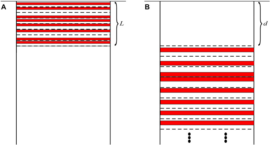
FIGURE 4. (A) $Cf\left(0,L,\theta \right)$ and (B) $Cf\left(d,\infty ,\theta \right)$.

Formula 9 shows that the deformation produced by the coupling fraction is equal to the sum of the SB73 model and $Cf\left(0,d,1-\delta \right)$. The equation $\theta =1-\delta =\frac{S_c}{S}$ illustrates that the CF model explains the coupling fraction well because $\theta$ represents the ratio of the creeping part of the fault segment. Therefore, based on the CF model, $\delta$ can be interpreted as the ratio of the total length of discontinuous locking parts in $Cf\left(d,L,\theta \right)$ to L (the correlation between $\theta$ and $\delta$ in layered faults is discussed in the Supplementary Material).

2.4 Model with depth-dependent decoupled fraction

Based on the CF model, the model of the fault with a $\theta$ value varying in depth was studied (VDFD model). The model with $\theta$ varying in depth is shown in Figure 5. It can be divided into patches: $\left[L_0,L_1\right],\left[L_1,L_2\right],\cdots \left[L_{n-1},L_n\right],\cdots .L_0=0$. The decoupled fraction is ${\theta }_{dp-i}$ in patch $\left[L_{i-1},L_i\right]$, $i=1,2\cdots n$. Based on the CF model, the total deformation generated by patches is presented as follows:

${\mathit{s}}_{\mathit{t}\mathit{o}\mathit{t}\mathit{a}\mathit{l}}\left(\mathit{x}\right)=\frac{\mathit{s}}{\mathit{\pi }}\bullet {\displaystyle \sum }_{\mathit{i}=\mathbf{1}}^{\mathit{n}}{\mathit{\theta }}_{\mathit{d}\mathit{p}-\mathit{i}}\bullet \left[{\mathit{tan}}^{-\mathbf{1}}\left(\frac{\mathit{x}}{{\mathit{L}}_{\mathit{i}-\mathbf{1}}}\right)-{\mathit{tan}}^{-\mathbf{1}}\left(\frac{\mathit{x}}{{\mathit{L}}_{\mathit{i}}}\right)\right].$

FIGURE 5

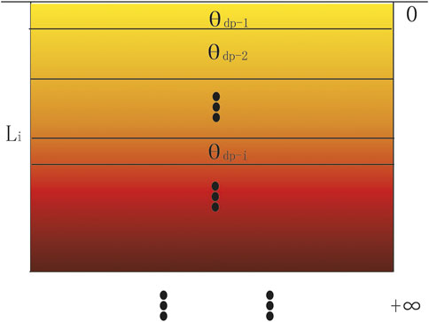
FIGURE 5. Model of the strike-slip fault with a depth-dependent $\theta$ value.

We then applied the Lagrange mean value theorem, $\forall i$, as follows:

${\mathit{s}}_{\mathit{t}\mathit{o}\mathit{t}\mathit{a}\mathit{l}}\left(\mathit{x}\right)=-\frac{\mathit{s}}{\mathit{\pi }}\bullet {\displaystyle \sum }_{\mathit{i}=\mathbf{1}}^{\mathit{n}}{\mathit{\theta }}_{\mathit{d}\mathit{p}-\mathit{i}}\bullet {\left.\frac{\mathit{d}{\mathit{tan}}^{-\mathbf{1}}\left(\frac{\mathit{x}}{\mathit{l}}\right)}{\mathit{d}\mathit{l}}\right|}_{\mathit{l}={\mathit{l}}_{{\mathit{\xi }}_{\mathit{i}}}}\bullet \left({\mathit{L}}_{\mathit{i}}-{\mathit{L}}_{\mathit{i}-\mathbf{1}}\right){\mathit{l}}_{{\mathit{\xi }}_{\mathit{i}}}\mathit{ϵ}\left[{\mathit{L}}_{\mathit{i}-\mathbf{1}},{\mathit{L}}_{\mathit{i}}\right].$

When ${\theta }_{dp-i}$ continuously varies with depth, ${\theta }_{dp-i}\left(i=1,2\cdots n\right)\Rightarrow \theta \left(l\right)$, the length of each patch is very small, that is, $n\to \infty$:

${\mathit{s}}_{\mathit{t}\mathit{o}\mathit{t}\mathit{a}\mathit{l}}\left(\mathit{x}\right)=\underset{\mathit{n}\to \infty }{\mathbf{lim}}-\frac{\mathit{s}}{\mathit{\pi }}\bullet {\displaystyle \sum }_{\mathit{i}=\mathbf{1}}^{\mathit{n}}{\mathit{\theta }}_{\mathit{d}\mathit{p}-\mathit{i}}\bullet {\left.\frac{\mathit{d}{\mathit{tan}}^{-\mathbf{1}}\left(\frac{\mathit{x}}{\mathit{l}}\right)}{\mathit{d}\mathit{l}}\right|}_{\mathit{l}={\mathit{l}}_{{\mathit{\xi }}_{\mathit{i}}}}\bullet \left({\mathit{L}}_{\mathit{i}}-{\mathit{L}}_{\mathit{i}-\mathbf{1}}\right).$

Therefore, the deformation of the VDFD model can be expressed as follows:

${\mathit{s}}_{\mathit{t}\mathit{o}\mathit{t}\mathit{a}\mathit{l}}\left(\mathit{x}\right)=\frac{\mathit{s}}{\mathit{\pi }}{\int }_{\mathbf{0}}^{+\mathit{\infty }}\frac{\mathit{\theta }\left(\mathit{l}\right)\bullet \mathit{x}}{{\mathit{x}}^{\mathbf{2}}+{\mathit{l}}^{\mathbf{2}}}\mathit{d}\mathit{l},(10)$

where s is the free slip rate, x is the distance from the fault, and l is the vertical distance from a certain depth to the surface. The $\theta \left(l\right)$ represents the function of $\theta$ with respect to l, where $0\le \theta \left(l\right)\le 1$. We defined the function of the coupling fraction with respect to l as $\delta \left(l\right)=1-\theta \left(l\right)$. The equation of $s_{total}\left(x\right)$ is similar to the distributed slip (Aki and Richards, 1980; Matthews and Segall, 1993). $s_{total}\left(x\right)$ is derived from the CF model, and $\theta \left(l\right)$ has a clear physical meaning. The critical function $\theta \left(l\right)$ controls the slip distribution of the fault. In this study, several examples of $\theta \left(l\right)$ and the corresponding deformation are provided (Figure 6). Figure 6A indicates that $\theta \left(l\right)$ gradually increases from the surface to the underground. Figure 6C indicates that $\theta \left(l\right)$ is fully locked above 30 km and fully creeping under 30 km, representing the SB73 model with a locking depth of 30 km. Figure 6E shows the fluctuation of $\theta \left(l\right)$ from the surface to the underground. Figures 6B, D, F show the corresponding curves. The VDFD model, which has a flexible $\theta \left(l\right)$, can produce more complex slip distributions than the SB73 and CF models.

FIGURE 6

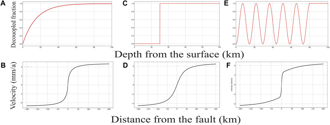
FIGURE 6. Examples of $\theta \left(l\right)$ values and the corresponding deformation. (A) $\theta \left(l\right)$ increases from the surface to underground 80 km; (C) $\theta \left(l\right)$ is 0 above 30 km and 1 below 30 km, which is the SB73 model; (E) $\theta \left(l\right)$ fluctuates from the surface to 80 km; (B,D,F) corresponding surface deformation. The shape of curve (B) is similar to the arctangent curve.

3 Discussion

3.1 Why is the shape of the coupling fraction deformation curve, which decreases with depth, similar to that of the arctangent curve?

The decrease in the coupling fraction with depth means that the decoupled fraction increases with depth. This study discusses the reason for the similar shapes of the curves for the arctangent function and decoupled fraction, which increase with depth. As shown in Figure 7, the decoupled fraction increases from the surface to d and is fully creeping below d, which is equal to the sum of faults B and C (Figure 7). Fault C is the SB73 fault, which generates the arctangent curve. Based on the CF model, the fault segment near the surface, which should produce large deformation, generates small deformation because of the small decoupled fraction in fault B. Hence, fault C dominates the shape of the whole curve. Therefore, the curve of fault A is similar to the arctangent curve.

FIGURE 7

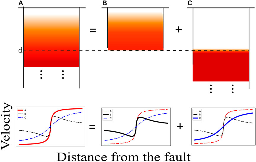
FIGURE 7. Schematic of the superposition of the decoupled fraction, which increases with depth; fault A = fault B + fault C. The corresponding deformation satisfies the equation. Red, black, and blue lines represent the deformation of faults (A, B, and C,) respectively.

3.2 Correlation among the coupling fraction, locking depth, and value of the locking depth based on curve fitting

Locking depth is the parameter in the SB73 model, which considers full coupling above the depth and full creeping below the depth. The curve produced by the SB73 model is an arctangent function. The coupling fraction $\delta$, which changes between 0 and 1, varies with depth. When $\delta$ is 1 above a certain depth $d_0$ and 0 below the $d_0$, then the $d_0$ can be considered the locking depth in the SB73 model. Sometimes the curves produced by the coupling fraction are similar to arctangent curves (Figure 7). By fitting curves that approximate the arctangent function with the SB73 model, we can obtain a value of the locking depth. The value reflects the average variation of the coupling fraction with depth. The quantitative correlation must be further studied.

3.3 Correlation between the deformation caused by step $\mathit{\theta }\left(\mathit{l}\right)$ and continuous $\mathit{\theta }\left(\mathit{l}\right)$

When inverting the coupling fraction on the fault, the fault plane is generally divided into many small patches, and the coupling fraction on each patch is a constant equivalent to replacing the continuous coupling fractions in practice with step ones. In this study, the correlation between the deformation caused by step $\theta \left(l\right)$ and continuous $\theta \left(l\right)$ in two dimensions is discussed based on the VDFD model. Based on Section 2.4, Formula 10 means the mapping from $\theta \left(l\right)$ to $s_{total}\left(x\right)$. The mapping is proven to have mathematical continuity and uniqueness (proof is provided in the Supplementary Material). Uniqueness means that there are no two different values of $\theta \left(l\right)$ that produce the same $s_{total}\left(x\right)$, which shows that there are no multiple solutions in theory. Continuity means that if ${\theta }_1\left(l\right)$ and ${\theta }_2\left(l\right)$ are similar, then $s_{total-1}\left(x\right)$ and $s_{total-2}\left(x\right)$ are also similar.

As shown in Figures 8A, C, the step $\theta \left(l\right)$ is used to replace the continuous $\theta \left(l\right)$. Figures 8B, D illustrate the difference between the deformations based on step $\theta \left(l\right)$ and continuous $\theta \left(l\right)$. The number of steps in Figure 8C is higher than that in Figure 8A, which is closer to the continuous $\theta \left(l\right)$. Therefore, the curve based on step $\theta \left(l\right)$ in Figure 8C is closer to that based on continuous $\theta \left(l\right)$, compared with that in Figure 8A. Thus, more steps yield results closer to the actual $\theta \left(l\right)$ but also indicate more unknown numbers with respect to the inversion. Therefore, the dense layout of global positioning system (GPS) stations can increase the data density of deformation, helping to improve the accuracy of the inversion of the coupling fraction, which may be hard to achieve at present because of the lack of sufficient GPS stations for some strike-slip faults. Three-dimensional models can be more complex because of lateral heterogeneity, which must be further studied.

FIGURE 8

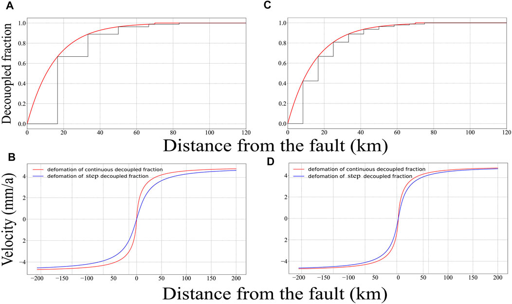
FIGURE 8. Deformation of step $\theta \left(l\right)$ approaching continuous $\theta \left(l\right)$. (A,C) Step $\theta \left(l\right)$ (black line) approaching continuous $\theta \left(l\right)$ (red line) with different steps. (B,D) corresponding deformation. Red and blue lines are based on continuous $\theta \left(l\right)$ and step $\theta \left(l\right)$, respectively.

3.4 Physical meaning of the coupling fraction

The CF model is obtained from the SB73 model and the superposition principle. Therefore, its mathematical correctness is guaranteed. One aim of this study was to explain the physical meaning of the coupling fraction. Based on the aforementioned discussion, we know that locking segments in the CF model could be tiny, numerous, and alternating with creeping segments. Based on microscopic and macroscopic views of the fault, fully coupled fault segments and non-fully coupled ones exist, respectively. The fault plane contains small and large asperities. Based on the magnitude–frequency correlation, it is known that the smaller the size, the greater is the number of asperities. Therefore, small asperities are widely distributed on the fault plane. The results of the numerical simulation show that the effect of an asperity impeding the creep of the fault diminishes by ∼90% when the distance is larger than 3–5 times the size of the asperity (Figures 9A, B). The fault plane contains numerous small asperities, which are all at certain distances from each other and impede each other’s motion. Although impediments lead to full coupling in local areas containing small asperities (e.g., black dashed box in Figure 9D), numerous impediments reduce the slip rate of the whole fault plane and the coupling fraction forms macroscopically. The test board results also show that when patches are very small, the alternate creeping and locking patches can also produce arctangent curves macroscopically (Figures 10A, B). Thus, the macroscopic fault slip rate should be less than that of the local area. Therefore, the fault slip rate obtained from repeating events (which may be closer to the free slip rate) is often greater than that based on the GPS velocity field (Li et al., 2011; Zhang et al., 2022). The physical meaning of the coupling fraction is the ratio of the total area of the small asperities to the fault area when the small asperities are distributed everywhere.

FIGURE 9

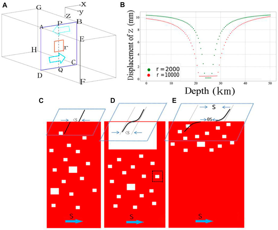
FIGURE 9. (A) Numerical simulation of the effect of asperity impediment using the three-dimensional (3D) numerical manifold method (NMM), which is useful for the simulation of discontinuous deformation as fault motion (Shi 2001; Wu et al., 2020). First, we set up a 3D research area and confining pressure. Subsequently, we pushed (two blue arrows) in opposite directions (AEFD inward and BGHC outward). The red-lined box represents an asperity; the side length is r. The displacement of the push is 10 mm. A row of measuring points PQ line was set up in ABCD. (B) Vertical deformation of the measuring points; the deformation for a side length of the asperity of 2000 m is represented by the green dashed line; the deformation for a side length of the asperity of 10,000 m is represented by the red dashed line. (C) S means the free slip rate. Small and numerous asperities without large asperities, <s means the value of creeping rate is smaller than the free slip rate S; (D) small and numerous asperities in the lower part and a huge asperity on the top part of the fault; (E) small and numerous asperities on the top part of the fault.

FIGURE 10

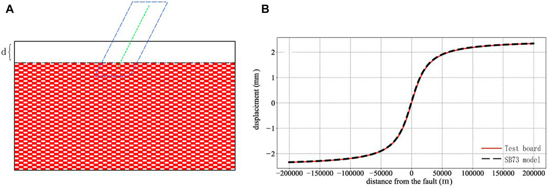
FIGURE 10. Results of test board fault. When the number of patches is $100\times 100=10000$, the deformation curve is very close to the arctangent function. (A) Test board fault; green dash line means measurement points, $s=10\mathrm{m}\mathrm{m}/\mathrm{a}$ and $d=20\mathrm{k}\mathrm{m}$; (B) curve made by the test board fault and the SB73 model with $s=5\mathrm{m}\mathrm{m}/\mathrm{a}$ and $d=20\mathrm{k}\mathrm{m}$.

Based on Section 2.2, we know that $1-\theta$ represents the ratio of the total area of numerous small asperities on the fault plane to their surrounding areas. The creeping rate of the fault with $s$ becomes smaller than $s$ because of many small asperities. If the fault plane contains numerous small but no large asperities, the fault creeps at a rate smaller than $s$ (Figure 9C). If the lower part of the fault contains many small asperities and the top part contains a giant asperity, the deformation is equivalent to that of the SB73 model with a slip rate smaller than $s$ (Figure 9D). If the top of the fault contains a large number of small asperities and no asperity is observed in the lower part, the deformation is the sum of the SB73 model and $Cf\left(0,L,\theta \right)$, the step interval is $\theta s$, and the slip rate is $s$ (Figure 9E). The large asperity and many small asperities determine the characteristics of surface deformation, but no matter how the small asperities are distributed, the far-field slip rate is often smaller than the free slip rate, $s$. The size of asperities is not infinitesimal, so the physical model is not the same as the mathematical model. The random positions of the asperities affect the shape of the deformation curve, which is similar but not identical to the arctangent curve (Figure 3). Therefore, it is possible that the surface deformation curve produced by a non-fully coupled strike-slip fault deviates from the arctangent curve. We can only approximate the shape of the arctangent curve because the distributions of a huge number of small asperities with certain sizes on the fault plane are unknown. In addition, limitations of this study exist due to the current models: 1) the models mentioned in this study are based on semi-infinite elastic bodies, so the transverse inhomogeneity and the influence of viscoelastic bodies are not considered in the models, and 2) the positions of creeping segments are random but laid on a relatively small range (Figure 2B), and the segment length of creeping segments is equal. In practice, the segment length of the creeping segments should be unequal and the positions should be more random. These problems are closer to reality and must be further studied in the future. Based on the aforementioned discussion, we have known that the far-field slip rate of the fault (or the secular slip rate) could often be smaller than the free slip rate. We could only obtain the secular/far-field slip rate by GPS velocity. The terms “secular/far-field slip rate of fault” and “free slip rate” should be distinguished.

4 Conclusion

Based on the SB73 model and the superposition principle, a CF model of the motion of non-fully coupled strike-slip faults was constructed using numerous tiny, alternating creeping and locking segments. The slip rate of the deformation produced by the CF model is $\theta s$, where $s$ is the free slip rate. The definition of the coupling fraction $\delta$ is interpreted by the CF model. A VDFD model is proposed based on the CF model. The models with non-fully coupled strike-slip faults provide insights into the complexity of the motion of strike-slip faults: 1) the surface deformation is generated by the fault slip rate $s$ with numerous small asperities, but the shape is equal to that of the deformation based on a lower slip rate $\theta s$ without asperities; 2) the meaning of the coupling fraction is the ratio of the total area of the small asperities to the fault area when the small asperities are widely distributed; and 3) according to the VDFD model, the curve generated by the non-SB73 model is sometimes similar to an arctangent curve. The CF and VDFD models provide deep cognition for understanding the deformation characteristics of non-fully coupled faults.

Data availability statement

The original contributions presented in the study are included in the article/Supplementary Material, further inquiries can be directed to the corresponding author.

Author contributions

Methodology, ZZ and ZJ; resources, ZZ; funding, ZZ, YW, and YC; test, ZZ; numerical simulation, ZZ and YW; visualization, ZZ; first draft preparation, ZZ and YC; editing, ZZ and YC; supervision, ZJ; proof, ZZ and HT.

Funding

This research was supported by the National Natural Science Foundation of China (41904092 and 41974011), the National Key Research and Development Program of China (2018YFE0109700 and 2019YFC1509203), and the Basic Research Project of the Institute of Earthquake Forecasting, China Earthquake Administration (2020IEF0506).

Acknowledgments

The authors express their gratitude to Tai Liu, Zhenyu Wang, and Yueyi Xu at the Institute of Earthquake Forecasting, China Earthquake Administration, and Long Zhang at the Institute of Geophysics, China Earthquake Administration, for their helpful discussions about the CF and VDFD models. The researcher YW in First Crust Monitoring and Application, China Earthquake Administration, provided the 3D-NMM calculation program. The authors also thank moderators Czhang271828, zhan-xun, kuing, and TSC999 on the online mathematics forum at http://kuing.infinityfreeapp.com/forum.php for their help with the core ideas of the proofs. Python and MATLAB software were used for numerical simulation and to prepare some of the figures.

Conflict of interest

The authors declare that the research was conducted in the absence of any commercial or financial relationships that could be construed as a potential conflict of interest.

Publisher’s note

All claims expressed in this article are solely those of the authors and do not necessarily represent those of their affiliated organizations, or those of the publisher, the editors and the reviewers. Any product that may be evaluated in this article, or claim that may be made by its manufacturer, is not guaranteed or endorsed by the publisher.

Supplementary material

The Supplementary Material for this article can be found online at: https://www.frontiersin.org/articles/10.3389/feart.2023.1059300/full#supplementary-material

References

Aki, K., and Richards, P. (1980). Quantitative seismology, 1. New York: W. H. Freeman.

Google Scholar

Chinnery, M. (1963). The stress changes that accompany strike-slip faulting. Bull. Seismol. Soc. Am. 53, 921–932. doi:10.1785/bssa0530050921

CrossRef Full Text | Google Scholar

Dong, J., Cheng, P., Wen, H., and Sun, W. (2021). Internal co-seismic displacement and strain changes inside a homogeneous spherical Earth. Geophys. J. Int. 225, 1378–1391. doi:10.1093/gji/ggab032

CrossRef Full Text | Google Scholar

Jian, H., Gong, W., Li, Y., and Wang, L. (2022). Bayesian inference of fault slip and coupling along the tuosuo lake segment of the kunlun fault, China. Geophys. Res. Lett. 49, e2021GL096882. doi:10.1029/2021GL096882

CrossRef Full Text | Google Scholar

Jiang, G., Xu, X., Chen, G., Liu, Y., Fukahata, Y., Wang, H., et al. (2015). Geodetic imaging of potential seismogenic asperities on the Xianshuihe-Anninghe-Zemuhe fault system, southwest China, with a new 3-D viscoelastic interseismic coupling model. J. Geophys. Res. -sol Ea. 120, 1855–1873. doi:10.1002/2014JB011492

CrossRef Full Text | Google Scholar

Li, L., Chen, Q., Niu, F., and Su, J. (2011). Deep slip rates along the Longmen Shan fault zone estimated from repeating microearthquakes. J. Geophys. Res. -sol Ea. 116, B09310. doi:10.1029/2011JB008406

CrossRef Full Text | Google Scholar

Li, L., Wu, Y., Li, Y., Zhan, W., and Liu, X. (2022). Dynamic deformation and fault locking of the xianshuihe fault zone, southeastern Tibetan plateau: Implications for seismic hazards. Earth Planets Space 74, 35. doi:10.1186/s40623-022-01591-9

CrossRef Full Text | Google Scholar

Li, Y., Hao, M., Song, S., Zhu, L., Cui, D., Zhuang, W., et al. (2021a). Interseismic fault slip deficit and coupling distributions on the Anninghe-Zemuhe-Daliangshan-Xiaojiang fault zone, southeastern Tibetan Plateau, based on GPS measurements. J. Asian Earth Sci. 219, 104899. doi:10.1016/j.jseaes.2021.104899

CrossRef Full Text | Google Scholar

Li, Y., Nocquet, J., Shan, X., and Jian, H. (2021b). Heterogeneous interseismic coupling along the xianshuihe-xiaojiang fault system, eastern tibet. J. Geophys. Res. -sol Ea. 126, e2020JB021187. doi:10.1029/2020JB021187

CrossRef Full Text | Google Scholar

Matsu’ura, M., Jackson, D., and Cheng, A. (1986). Dislocation model for aseismic crustal deformation at Hollister, California. J. Geophys. Res. -sol Ea. 91, 12661–12674. doi:10.1029/JB091iB12p12661

CrossRef Full Text | Google Scholar

Matthews, M., and Segall, P. (1993). Estimation of depth-dependent fault slip from measured surface deformation with application to the 1906 San Francisco Earthquake. J. Geophys. Res. 98, 12153–12163. doi:10.1029/93JB00440

CrossRef Full Text | Google Scholar

McCaffrey, R. (2005). Block kinematics of the Pacific–North America plate boundary in the southwestern United States from inversion of GPS, seismological, and geologic data. J. Geophys. Res. 110, B07401. doi:10.1029/2004JB003307

CrossRef Full Text | Google Scholar

McCaffrey, R. (2002). “Crustal block rotations and plate coupling,” in Plate boundary zones. Editors S. Stein, and J. T. Freymueller (Washington D.C.: Geodynamics Series), 101–122.

Google Scholar

McCaffrey, R., Long, M., Goldfinger, C., Zwick, P., Nabelek, J., Johnson, C., et al. (2000). Rotation and plate locking at the southern cascadia subduction zone. Geophys. Res. Lett. 27, 3117–3120. doi:10.1029/2000GL011768

CrossRef Full Text | Google Scholar

Okada, Y. (1992). Internal deformation due to shear and tensile faults in a half-space. Bull. Seism. Soc. Am. 82, 1 018–1040. doi:10.1785/BSSA0820021018

CrossRef Full Text | Google Scholar

Okada, Y. (1985). Surface deformation due to shear and tensile faults in a half-space. Bull. Seism. Soc. Am. 75, 1135–1154. doi:10.1785/BSSA0750041135

CrossRef Full Text | Google Scholar

Pan, E. (2019). Green’s functions for geophysics: A review. Rep. Prog. Phys. 82, 106801. doi:10.1088/1361-6633/ab1877

PubMed Abstract | CrossRef Full Text | Google Scholar

Reid, H. (1910). “The machanism of the earthquake,” in The California Earthquake of april 18, 1906 (Washington, D.C: Report of the State Earthquake Investigation Commission), 2.

Google Scholar

Savage, J., and Burford, R. (1973). Geodetic determination of relative plate motion in central California. J. Geophys. Res. 78, 832–845. doi:10.1029/JB078i005p00832

CrossRef Full Text | Google Scholar

Savage, J. (1990). Equivalent strike-slip earthquake cycles in half-space and lithosphere-asthenosphere Earth models. J. Geophys. Res. -sol Ea. 95, 4873–4879. doi:10.1029/JB095iB04p04873

CrossRef Full Text | Google Scholar

Scholz, C. H (2007). The mechanics of earthquakes and faulting. Environ. Eng. Geoscience - ENVIRON ENG GEOSCI 13, 81–83. doi:10.2113/gseegeosci.13.1.81

CrossRef Full Text | Google Scholar

Segall, P. (2010). Earthquake and volcano deformation. New Jersey, United States: Princeton University Press. doi:10.1515/9781400833856

CrossRef Full Text | Google Scholar

Shi, G. (2001). “Three dimensional discontinuous deformation analysis,” in Proceedings of // International Conference on Analysis of Discontinuous Deformation, Glasgow, Scotland, UK, 6th - 8th June 2001, 1–21.

Google Scholar

Steketee, J. (1958). On volterra’’s dislocations in a semi-infinite elastic medium. Can. J. Phys. 36, 192–205. doi:10.1139/p58-024

CrossRef Full Text | Google Scholar

Sun, W., and Okubo, S. (1998). Surface potential and gravity changes due to internal dislocations in a spherical Earth—ii. Application to a finite fault. Geophys. J. Int. 132, 79–88. doi:10.1046/j.1365-246x.1998.00400.x

CrossRef Full Text | Google Scholar

Sun, W., and Okubo, S. (1993). Surface potential and gravity changes due to internal dislocations in a spherical Earth—I. Theory for a point dislocation. Geophys. J. Int. 114, 569–592. doi:10.1111/j.1365-246X.1993.tb06988.x

CrossRef Full Text | Google Scholar

Wang, R., Martin, F., and Roth, F. (2003). Computation of deformation induced by earthquakes in a multi-layered elastic crust—FORTRAN programs EDGRN/EDCMP. Comput. Geosci-Uk. 29, 195–207. doi:10.1016/S0098-3004(02)00111-5

CrossRef Full Text | Google Scholar

Wu, Y., Chen, G., Jiang, Z., Zhang, H., Zheng, L., Pang, Y., et al. (2020). Three dimensional numerical manifold method based on viscoelastic constitutive relation. Int. J. Geomech. 20. doi:10.1061/(ASCE)GM.1943-5622.0001798

CrossRef Full Text | Google Scholar

Zhang, L., Su, J., Wang, W., Fang, L., and Wu, J. (2022). Deep fault slip characteristics in the Xianshuihe-Anninghe-Daliangshan Fault junction region (eastern Tibet) revealed by repeating micro-earthquakes. J. Asian Earth Sci. 227, 105115. doi:10.1016/j.jseaes.2022.105115

CrossRef Full Text | Google Scholar

Zhao, J., Ren, J., Liu, J., Jiang, Z., Liu, X., Liang, H., et al. (2020). Coupling fraction and relocking process of the longmenshan fault zone following the 2008 Mw7.9 wenchuan earthquake. J. Geodyn. 137, 101730. doi:10.1016/j.jog.2020.101730

CrossRef Full Text | Google Scholar