Establishment of Wind Gust Estimation Equation in Bohai Sea

Wind gusts over the ocean can have a great influence on maritime transport and production operations. However, owing to the scarcity of marine observation data and the complex causes of wind gusts, the estimation and forecasting of gusts at sea are even more difficult. In this study, a gust estimation equation applicable to the Bohai Sea is established based on observation and reanalysis data, with representative observation stations on the coast and offshore in the Bohai Sea. During the process, partial correlation analysis and a significance test of correlation coefficient differences were used to further clarify the influence of average wind speed and vertical wind shear at different heights on wind gusts. The final gust estimation equation includes a mean wind speed term, a turbulence term, and a convection term, which are statistically significant contributors; in addition, there are clear physical meanings. Comparing two gust factor methods in this study, the average errors and fitting errors of the least squares gust estimation equation are the smallest. For wind gusts between 10 and 26 m/s, the fitting error in the gust estimation equation is 7.68–12.25% and 21.10–30.08% lower than those of the two gust factor methods in this study. The gust estimation equation better reflects the difference of wind gusts typical under different average wind speeds and vertical wind shear conditions, so a better prediction for wind gusts can be achieved.

Introduction

Wind gusts are strong, short-duration wind events that are measured by the average wind speed over several seconds. Wind gusts exceeding a certain threshold have a significant impact on housing, transportation, and/or maritime production (Sheridan, 2018; Teoh et al., 2019; Su et al., 2021). Accurate and timely wind gust forecast information can effectively reduce the loss of life and property. The formation mechanism of wind gusts is complex and is not only related to average wind speed and boundary layer turbulence but also affected by surface roughness and atmospheric stability (Harris and Kahl, 2017). For this reason, the prediction of wind gusts is a difficult problem in operational weather forecasting (Kahl, 2020). The wind gust factor was an early wind gust forecasting metric that was calculated as the ratio of the maximum wind speed to the average wind speed within a set time period. From this metric, the strength of wind speed pulsation was obtained, and the expected maximum wind gust value was estimated (Sherlock, 1952). The wind gust factor methodology is still widely used in practical operational forecasting owing to its simplicity and convenience (Cook et al., 2008; Blaes et al., 2014). However, because of the influence of different underlying surface conditions, altitude, and weather systems, the wind gust factor varies significantly. Therefore, in order to obtain more accurate wind gust forecasts, there has been considerable research on the factors driving wind gusts (Davis and Newstein, 1968; Krayer and Marshall, 1992; Ágústsson and Ólafsson, 2004; Yu and Chowdhury, 2009; Kahl et al., 2021). The wind gust factor methodology considers only the general relationship between the average wind speed and wind gusts and ignores the effects of the vertical distribution of upper-level wind speeds on surface wind gusts. When the vertical wind shear near the surface is large, strong turbulent momentum flux will occur, and this strong turbulent momentum flux will increase the surface wind gusts. Strong vertical wind shear in the troposphere is conducive to the development of convective weather, and when convective weather occurs, downdrafts in the troposphere reach the surface, thereby increasing the surface wind gusts (Brasseur, 2001; ECMWF, 2016; Minola et al., 2020). Therefore, by considering the effects of turbulence and convection on the average surface wind speed, which the wind gust factor method ignores, more accurate wind gust predictions can be obtained.

Compared with the average wind speed, strong wind gusts offshore have a greater impact on the safety of both maritime shipping and offshore production operations. However, the lack of observational data at sea, either high-altitude observations or ground-level observations, limits the accurate representation of the initial marine meteorological conditions in numerical models. This restricts the development of objective forecasting methods over the oceans. However, the underlying conditions at the sea surface are relatively uniform, which provides favorable conditions for the development of wind gust forecasting at sea (Leston et al., 2018).

The Bohai Sea is a relatively small inland sea in northern China, which has a substantial network of in situ observing sites, such as coastal observation sites, buoys, and oil platforms. Therefore, this study will use the gusts and mean wind observation data of these stations and the upper-air wind field data from reanalysis data to establish a gust estimation model that can be applied to the Bohai Sea. Through this model, the wind gusts can be more accurately estimated for varying average wind speeds and vertical wind shear conditions to provide a new method for wind gust forecasting in the Bohai Sea.

Data

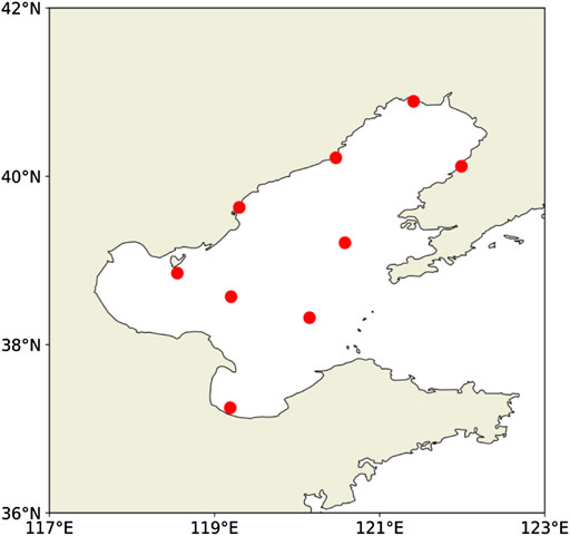
In this article, we use hourly wind speed data from surface observations taken by the China Meteorological Administration during 2017–2019 and wind field data on 1,000, 925, and 850 hPa from the ERA5 reanalysis data to establish an hourly wind gust forecast model for the Bohai Sea. The spatial resolution of the ERA5 reanalysis data is 0.25 × 0.25. A bilinear interpolation method is used to interpolate the upper-air data to the locations of the selected coastal and representative offshore stations shown in Figure 1. There are nine representative stations selected from the coastal and offshore areas in this study. The average elevation of the selected stations is 10 m, so the wind speed observation data do not need to be corrected in height. When using wind speed data to calculate wind gusts, the wind speed should be averaged over a 10-min interval (Harper et al., 2010; WMO, 2012). However, the numerical prediction model used in weather forecasting mainly outputs the wind speed at the forecast time. Therefore, in order to apply the established wind gust estimation equation in operational forecasting in the future, the average wind speed at the observation time is used instead of the 10-min average wind speed. In this study, it is a 2-min average and is recorded as integer values.

FIGURE 1

FIGURE 1. The distribution of representative stations in coastal and offshore areas.

Factor Analysis

In general, the speed of wind gusts rises with the increase of the average wind speed. The observational data from 2017 to 2019 show that when the average wind speed is between 14 and 16 m/s, the corresponding average value of observed wind gusts is approximately 19 m/s, and when the average wind increases to 22–24 m/s, average wind gusts can reach 28 m/s. Since there is only one parameter, there is a direct relationship between the average wind speed and the gust prediction. However, in practice, different gusts can occur at any specific average wind speed (Figure 2). Therefore, as the average wind speed is an important factor in gust estimation, it alone is not an accurate predictor for the wind gust speed.

FIGURE 2

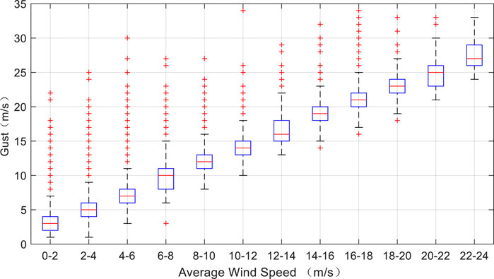
FIGURE 2. Boxplots of average wind speed and wind gust from 2017 to 2019. The boxplot corresponds to the minimum, 25th percentile, 50th percentile (red lines), 75th percentile, and maximum values from bottom to top, respectively. Red crosses in the figure represent outliers that are more than 1.5 quartiles away from the 75th percentile or 25th percentile of the box.

Turbulence is the main characteristic of the atmospheric boundary layer and plays an important role in the transfer of heat, momentum, and water vapor between the surface and the upper atmosphere (Gousseau et al., 2012). Strong vertical wind shear is conducive to the enhancement of turbulence (Kim et al., 2003). The height of 1,000 hPa is close to the ground, so this study attempts to use the difference between the wind speed of 1,000 hPa (F₁₀₀₀) and that at 10 m (F₁₀) to estimate the vertical wind shear in the near-ground layer. Figure 3 is an array boxplot of different average wind speeds from 2017 to 2019 under the conditions of F₁₀₀₀-F₁₀ > 0 and F₁₀₀₀-F₁₀ ≤ 0. As is shown in Figure 3, by comparing the gust distribution in the two cases, it can be seen that under the same average wind speed, the larger gust is more likely to appear in the case of F₁₀₀₀-F₁₀ > 0. The case of F₁₀₀₀-F₁₀ > 0 may correspond to a stronger turbulence, which would be associated with larger surface wind gusts.

FIGURE 3

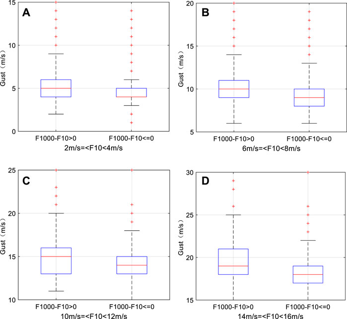
FIGURE 3. Boxplots of gusts under different average wind speeds when F1000-F10 > 0 and F1000-F10 ≤ 0 from 2017 to 2019: (A) 2 m/s ≤ F10 < 4 m/s; (B) 2 m/s ≤ F10 <4 m/s; (C) 2 m/s ≤ F10 < 4 m/s; and (D) 2 m/s ≤ F10 < 4 m/s.

When a severe convective weather system occurs, downdrafts in the troposphere will transport momentum downward and affect surface wind gusts. However, severe convective weather has the characteristics of small spatial scale, short life, and strong suddenness. The prediction of severe convective weather is still a difficult problem (Grabowski et al., 2019), and it is even more difficult to quantitatively calculate the surface gusts caused by severe convective weather. In the gust forecast product of the European Center for Medium-Range Weather Forecasts (ECMWF) model, the maximum positive wind speed difference between 850 and 950 hPa is used to represent the gust caused by convective weather, so as to realize the quantitative calculation of convective gust (ECMWF, 2016). In this study, the vertical wind shears between the 850- and 1,000-hPa surfaces (F₈₅₀-F₁₀₀₀) and between the 850 and 925-hPa surfaces (F₈₅₀-F₉₂₅) are used to characterize the effects of convection.

Correlation Analysis

Since the average surface wind speed and vertical wind shear both can affect the intensity of surface wind gusts, the relationship between them needs to be further clarified. The simple correlation coefficient only shows the degree of linear relation between two variables and does not fully clarify the relationship between those independent variables and the dependent variables in multiple regression analysis. Therefore, a partial correlation analysis needs to be performed, which considers other impact factors and temporarily ignores their influence, to study the relationship between the two remaining factors (Baka et al., 2004). When the partial correlation coefficient is first order, there are only two influence factors. The influence of one independent variable is being controlled, and the relationship between the other independent variable and the dependent variable is calculated according to the following (Hu and Wu, 2020):

$r_{ab\_c}=\frac{r_{ab}-r_{ac}{r}_{bc}}{\sqrt{\left(1-r_{ac}^2\right)\left(1-r_{bc}^2\right)}}(1)$

where $r_{ab\_c}$ is the partial correlation coefficient between dependent variable a and independent variable b when controlling the effect of the independent variable c, and $r_{ab}$, $r_{ac}$, and $r_{bc}$ are the simple correlation coefficients between a and b, a and c, and b and c, respectively. When there are three impact factors, it is necessary to control the influence of two of them to calculate the relationship between the remaining one and the dependent variable. Therefore, it is necessary to calculate the second-order partial correlation coefficient according to the following (Ashok et al., 2007):

$r_{ab\_cd}=\frac{r_{ab\_c}-r_{ad\_c}{r}_{bd\_c}}{\sqrt{\left(1-r_{ad\_c}^2\right)\left(1-r_{bd\_c}^2\right)}}(2)$

where $r_{ab\_cd}$ is the correlation between dependent variable a and independent variable b when controlling the effects of the independent variable c and d.

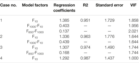
The vertical wind shear is divided into four cases, and the partial correlation coefficients of the wind shear variables under the four different vertical wind shear conditions from 2017 to 2019 are calculated. By using partial correlation analysis to compare the effects of F₈₅₀-F₉₂₅ and F₈₅₀-F₁₀₀₀ on surface gusts, it is found that the effects of F₈₅₀-F₉₂₅ is smaller than that of F₈₅₀-F₁₀₀₀ (not show), so F₈₅₀-F₁₀₀₀ is finally selected to represent the gust caused by convective weather (Table 1). The partial correlation coefficients in Table 1 are all significant at the 95% level. These results show that the partial correlation coefficient of the average wind speed is the largest regardless of the vertical wind shear conditions, indicating that the average wind speed is the most important factor affecting the surface wind gusts. When F₁₀₀₀-F₁₀ > 0, the partial correlation coefficients are 0.314 and 0.346 (Case 1 and Case 2), which are much larger than 0.072 and 0.135 when F₁₀₀₀-F₁₀ ≤ 0 (Case 3 and Case 4). When F₈₅₀-F₁₀₀₀ > 0 (Case 1 and Case 3), the partial correlation coefficients are 0.07 and 0.103, which are also greater than 0.016 and 0.02 when F₈₅₀-F₁₀₀₀ ≤ 0 (Case 2 and Case 4).

TABLE 1

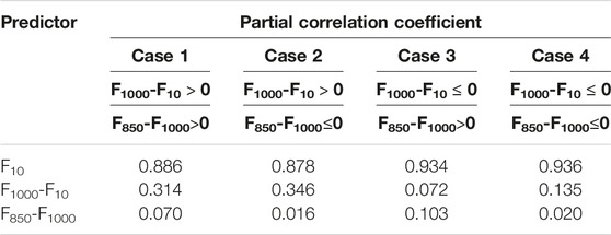
TABLE 1. Partial correlation coefficients of forecast factors under different vertical wind shear conditions from 2017 to 2019.

The partial correlation coefficients are calculated from the corresponding sample data. However, before comparing different correlation coefficients, a statistical test should be performed to make sure whether the difference between different correlation coefficients is statistically significant or possibly caused by sampling differences or random chance. In 1915, Fisher proposed the Fisher Z transform, which can convert correlation coefficients that do not conform to normal distribution into variables that conform to normal distribution (Needham, 1978). The formula is calculated as follows:

$z_r=\frac{1}{2}\ln \left(\frac{1+r_r}{1-r_r}\right)(3)$

where $r_r$ is the correlation coefficient of a sample data and $z_r$ is the transformed correlation coefficient. Using this transformed correlation coefficient, Snedecor (1980) proposed a method to test the differences between two correlation coefficients. The procedure is as follows: Define

$z=\frac{z_{r1}-z_{r2}}{VAR\left(z_{r1}-z_{r2}\right)}(4)$

where Z_r1 and Z_r2 are the transformed correlation coefficients and VAR(Z_r1–Z_r2) is calculated by the following:

$VAR\left(z_{r1}-z_{r2}\right)=\sqrt{\frac{1}{n_1-3}+\frac{1}{n_2-3}}(5)$

where n₁ and n₂ represent the sample sizes of variables z₁ and z₂ in the data, respectively. The numbers of samples under four different vertical wind shear conditions in this study are 85,453, 49,929, 24,365, and 10,333 (Case 1–Case 4, respectively). When the absolute value of Z exceeds 1.96, the differences in the correlation coefficients of the two variables are statistically significant at the 95% confidence level. When the absolute value of Z is less than 1.96, the correlation coefficients are not significantly different.

The above procedure is used to test the difference of correlation coefficients for the different vertical wind shear conditions. The results show that only two of the correlation coefficient differences are not statistically significant. The first is F₁₀ for the two cases where F₁₀₀₀-F₁₀ is nonpositive and the partial correlation coefficients are 0.934 and 0.936, and the second is F₈₅₀-F₁₀₀₀ for the two cases where F₁₀₀₀-F₁₀ is positive and the partial correlation coefficients are 0.016 and 0.020. The significance test shows that the correlation coefficient between different samples can be compared, and the larger the correlation coefficient is, the greater the influence on the gusts will be. When F₁₀₀₀-F₁₀ > 0, the impact of F₁₀₀₀-F₁₀ on gusts is greater than that of F₁₀₀₀-F₁₀ ≤ 0. The corresponding physical meaning of this correlation is likely related to the fact that the positive vertical wind shear in the near-ground layer can stimulate strong turbulence, thereby enhancing gusts. When F₈₅₀-F₁₀₀₀ is greater than 0, it also has a greater impact on gusts, and its corresponding physical meaning is that the positive vertical wind shear is more likely to cause downdrafts in the troposphere to affect the surface gusts.

Therefore, the influence of F₁₀₀₀-F₁₀ ≤ 0 and F₈₅₀-F₁₀₀₀ ≤ 0 will be ignored when establishing the gust estimation equation, and the equation established in this way has a clearer physical meaning. The influence of different factors on surface wind gusts is more clearly revealed using partial correlation analysis and the significance test of correlation coefficient differences, which provide a basis for the establishment of a wind gust estimation equation.

Estimation Equation

The multiple linear gust estimation equation established from a multiple regression analysis can be written in the form of a piecewise function, as follows:

$F_{gust}=\{\begin{array}{cc}{a}_1{F}_{10}+b_1\left(F_{1000}-F_{10}\right)+c_1\left(F_{850}-F_{1000}\right)& F_{1000}-F_{10}\text{>0};F_{850}-F_{1000}\text{>0}\\ a_2{F}_{10}+b_2\left(F_{1000}-F_{10}\right)& F_{1000}-F_{10}\text{>0;}{F}_{850}-F_{1000}\le 0\\ a_3{F}_{10}+c_3\left(F_{850}-F_{1000}\right)& F_{1000}-F_{10}\le \text{0;}{F}_{850}-F_{1000}\text{>0}\\ a_4{F}_{10}& F_{1000}-F_{10}\le \text{0;}{F}_{850}-F_{1000}\le \text{0}\end{array}(6)$

where $a_i$, $b_i$, and $c_i$ are the coefficients of the three different influencing factors under the $i\text{th}$ vertical wind shear condition. Using the least squares method to solve the regression coefficients, we obtain the results presented in Table 2. The problem of collinearity among predictors in multiple linear regressions is an unavoidable problem. Severe collinearity can affect the fitting and may even lead to erroneous conclusions. The variance inflation factor (VIF) is an important metric to test for collinearity among the predictors. It is generally considered that if VIF > 10, there is a serious collinearity problem among the predictors (Al-Ashkar et al., 2021). The formula for calculating VIF is as follows:

$VI{F}_i=\frac{1}{1-R_i^2}(7)$

where $R_i^2$ is the square of R of independent variable i and the remaining independent variables in the linear regression. It can be seen in Table 2 that the range of VIFs in the different forecasting models ranges from 1.0 to 2.021 $\ll$ 10, indicating that there are no serious collinearity problems for any of the forecasting factors. Therefore, the estimation equation can be fitted by using the least squares method, and there is no need to use either a partial least squares or ridge regression method to eliminate collinearity (Delsole, 2007; Smoliak et al., 2015; Lala et al., 2020).

TABLE 2

TABLE 2. Model overview.

As shown in Table 2, in the case when F₁₀₀₀-F₁₀ ≤ 0 and F₈₅₀-F₁₀₀₀ ≤ 0 (Case 4), the only significant influencing factor in the wind gust estimation equation is F₁₀. In this case, the R² of the estimation equation is 0.987, which is the largest of all estimation equations. R² is the goodness of fit, and the closer the value is to 1, the better the fitting effect is. In this case, only using F₁₀ as a predictor achieves a better forecast of the wind gusts, and the standard error of the estimated value is the smallest of all cases (1.437 m/s). When F₁₀₀₀-F₁₀ > 0 and F₈₅₀-F₁₀₀₀ > 0 (Case 1), there are three factors in the estimation equation. In this case, the $R^2$ of the gust estimation equation is the smallest (0.951). Among the four gust estimation equations, the average wind speed has influence with a regression coefficient ranging from 1.292 to 1.385. The regression coefficients of F₁₀₀₀-F₁₀ are 0.403 and 0.439, and the regression coefficients of F₈₅₀-F₁₀₀₀ are 0.168 and 0.137. The regression coefficient of any particular factor is not very sensitive to the specific wind shear case, so we integrated the piecewise functions to make the gust estimation equation more concise and easy to use for operational forecasts. The procedure adopted in this study is to replace all the data for F₁₀₀₀-F₁₀ ≤ 0 and F₈₅₀-F₁₀₀₀ ≤ 0 with 0, merge all the sample data together, and use the least squares method to re-solve the regression coefficients for the different influencing factors. The VIF values between the influencing factors in the combined data are 1.446, 1.408, and 1.344, so there is no serious collinearity problem between the factors. The $R^2$ of the integrated gust estimation equation is 0.963, and the standard error of the estimated value is 1.703 m/s. The coefficients in the integrated gust estimation equation are 1.332, 0.437, and 0.153, which are basically equivalent to the average values of the coefficients of different influence factors in formula 6(1.33, 0.421, and 0.153, respectively). The final form of the wind gust estimation equation is as follows:

$F_{gust}=1\text{.}332F_{10}+\text{0}\text{.}437\max \left(0,F_{1000}-F_{10}\right)+\text{0}\text{.}153\max \left(0,F_{850}-F_{1000}\right)(8)$

where $\max \left(0,F_{1000}-F_{10}\right)$ and $\max \left(0,F_{850}-F_{1000}\right)$ includes only positive values of F₁₀₀₀-F₁₀ and F₈₅₀-F₁₀₀₀, respectively.

The wind gust estimation equation involves the wind speed on the 1,000-hPa surface. However, when the height of the 1,000-hPa surface is less than 10 m, F₁₀₀₀-F₁₀ and F₈₅₀-F₁₀₀₀ have no real physical meaning. Therefore, in this study, when the height of the 1,000-hPa surface is less than 10 m, the 1,000-hPa surface height data from the ERA5 reanalysis data is used to calculate the relationship between the 1,000- and 850-hPa wind speeds and the 10-m wind speed. However, the situation when the height of the 1,000-hPa surface is below 10 m and F₁₀₀₀-F₁₀ is positive accounts for only ∼1.7% of all samples during 2017–2019, and the average value of F₁₀₀₀-F₁₀ is ∼1.95 m/s. This situation primarily occurs when F₁₀ is relatively small (1–3 m/s), with a frequency of roughly 51.6% of the time. The proportion of cases when the height of the 1,000-hPa surface is below 10 m and F₈₅₀-F₁₀₀₀ is positive is approximately 2.2%, of which roughly 64.7% of the magnitudes of F₈₅₀-F₁₀₀₀ are less than 5 m/s. In general, when the height of the 1000-hPa surface is below 10 m, F₁₀₀₀-F₁₀ and F₈₅₀-F₁₀₀₀ have relatively little meaning and have little effect on the wind gust estimates.

Perform Validations

In this study, according to the definition of the gust factor method, two wind gust factors are calculated using the hourly wind speed observation data from 2017 to 2019. The first is the gust factor calculated based on different average wind speeds (GF1), and the second is the gust factor calculated based on the overall sample (GF2). As shown in Figure 4, GF1 monotonically decreases with the increase of average wind speed. When the average wind speed is 0–2 m/s, GF1 is 3.6155. When the average wind speed increases to 22–24 m/s, GF1 is 1.2314. At each average wind speed, GF2 is 1.5.

FIGURE 4

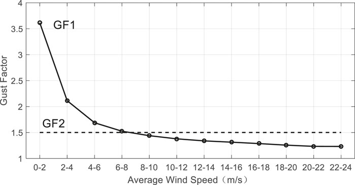
FIGURE 4. The gust factors as a function of average wind speed (GF1) and overall sample (GF2) calculated from the data from 2017 to 2019.

The gust estimation equation arising from the multiple regressions (MR) and the gust factors GF1 and GF2 are used to hind cast the data from 2017 to 2020 and compare their mean errors and fitting errors. The fitting error is estimated by the following:

$RMSE=\sqrt{\frac{1}{n}{\displaystyle \sum _{i=1}^n{\left(y_i-{\widehat{y}}_i\right)}^2}}(9)$

where $y_i$ is the observational wind gust data and ${\widehat{y}}_i$ is the hindcasted wind gusts from MR, GH1, or GF2. As is shown in Figure 5A, the amplitude of the mean error from MR is lower than that from GF1 at all wind gust speeds except 6–10 m/s. In some cases, the mean error from the MR is less than half that of GF1. When the wind gusts are above 10 m/s, the estimated value of the wind gusts estimated from GF1 are obviously smaller than the observed gusts, and the difference enlarges with the increase of wind gusts. When the observed gusts are 22–24, 24–26, and 26–28 m/s, the estimated gusts from GF1 are 32.9, 52.4, and 63% smaller, respectively, than the observed value by more than 2 m/s. The reduction in mean error in the MR model translates into a reduction in both the underestimation of strong wind gusts and the overestimation of low wind gusts. In comparison, the gust hindcasts from the GF2 model show a negative mean error for wind gusts below 14 m/s and a positive mean error when they are above 14 m/s. The estimations from the GF2 model are independent of the average wind speed, so the hindcasts are overestimates for weak wind gusts and underestimates for strong ones. Except in a few cases, the magnitude of the mean error of the MR model is smaller than that of the GF2 model (Figure 5B).

FIGURE 5

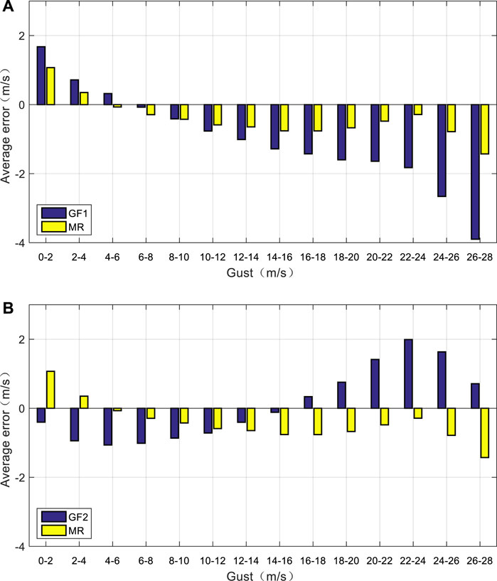
FIGURE 5. Comparison of mean error in the multiple regression model to that in the (A) gust factor and (B) gust factor 2 models from 2017 to 2019.

However, the mean error comparison does not prove that the estimation capability of the MR model is better than that of the GH1 or GF2 model. Table 3 shows the reduction of percentage in the fitting error of the MR model related to the fitting error in the GF1 and GF2 models. In Table 3, except when the observed wind gusts are between 2 and 4 m/s, the fitting error reduction rate of MR relative to that of the GF1 model is negative, and all others are positive. For wind gusts between 12 m/s and 22 m/s, the fitting error in the MR model is 10.99–12.25% lower than that of the GF1 model. For wind gusts between 4 and 26 m/s, the fitting error reduction of the MR model is more than 20% relative to that of the GF2 model.

TABLE 3

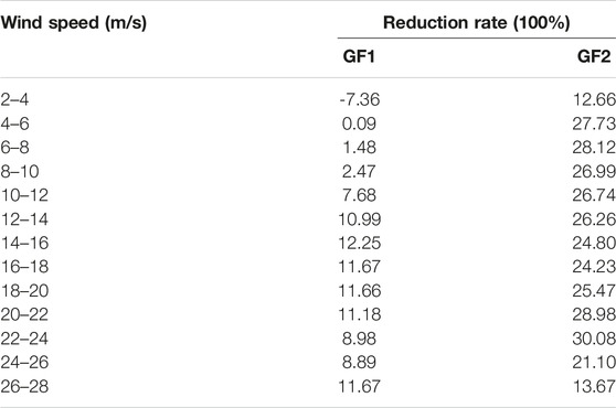
TABLE 3. Reduction rate of the multiple regression model relative to the gust factor 1 and gust factor 2 fitting error in 2017–2019.

Figure 6 shows the scatter diagrams of absolute errors of the MR and GF1 models. As can be seen, when the absolute error of GF1 is small, the absolute error of MR is also small, so that the scattered points near the origin are densely packed. As the absolute error of GF1 increases, the scattered points begin shifting to the left of the diagonal, indicating that the MR error is less than that in GF1. Figure 7 shows the scatter diagrams comparing the absolute error of the MR and GF2 models. The results in Figure 7 are basically the same as those in Figure 6; the absolute error in the MR model has fewer large deviations in the gust than the GF2 model does.

FIGURE 6

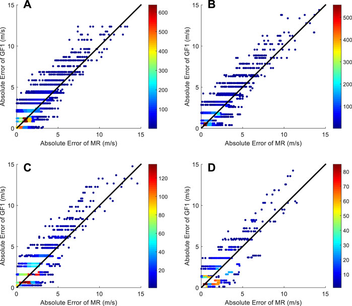
FIGURE 6. The scatter diagrams of absolute errors of the multiple regression method (MR) and the wind gust factor method (GF1) for four different observed gust magnitudes: (A) 14–16 m/s, (B) 16–18 m/s, (C) 18–20 m/s, (D) 20–22 m/s. The color in the scatter in the figure indicates the number of repeated scatter points.

FIGURE 7

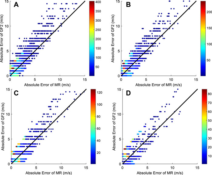
FIGURE 7. The scatter diagrams of absolute errors of the multiple regression method (MR) and the wind gust factor method (GF2) for four different observed gust magnitudes: (A) 14–16 m/s, (B) 16–18 m/s, (C) 18–20 m/s, (D) 20–22 m/s. The color in the scatter in the figure indicates the number of repeated scatter points.

By comparing the mean error, fitting error, and the scatter diagrams of the absolute error between the gust estimation equations method and the two gust factor methods, it is clear that the regression estimation equation is considerably better than the other two gust factor methods. This is because the regression considers both average wind speed and wind shear at different heights.

Summary and Discussion

In this study, based on both observational and ERA5 reanalysis data, the relationship among average wind speed, vertical wind shear at different levels in the lower atmosphere, and surface wind gusts is determined by the analysis of partial correlation and the development of wind gust estimation equation suitable for Bohai Sea using the least squares method. By comparing the gust estimation equation and the two gust coefficients, the results are as follows:

1. The average wind speed term F₁₀ and the wind shear terms F₁₀₀₀-F₁₀ and F₈₅₀-F₁₀₀₀ are selected to establish an estimation equation for wind gusts in the Bohai Sea. While average wind speed is the dominant factor in the surface wind gust estimation, the near-surface wind shear is also an important term. Owing to the low frequency and intermittency of convective weather systems, the effects of convection as estimated using the wind shear across 850–1,000 hPa are relatively small.

2. Based on the significance test of the correlation coefficient difference, it is clear that the positive vertical wind shear has a greater impact on the ground gust than the negative vertical wind shear. The gust estimation equation ultimately includes the importance of vertical wind shear, which is more physically meaningful.

3. Compared with the two gust factor methods presented in this study (GF1 and GF2), the mean error and fitting error of the least squares regression gust estimation equation (MR) are the smallest. For wind gusts between 10 and 26 m/s, the fitting error in the gust estimation equation is 7.68–12.25% and 21.10–30.08% lower than those of the two gust factor methods in this study. The least squares regression gust estimation equation includes the effects of the average wind speed and different vertical wind shear conditions, so a better prediction for the wind gusts can be achieved.

The surface 10-m wind speed and 1,000- and 850-hPa wind speed data predicted using the numerical model can be applied in the gust estimation equation to realize the gust forecast. In this study, the gust estimation equation was established based on the Bohai Sea. If the gust estimation equation is applied to other sea areas, it is necessary to reselect representative stations to calculate the regression coefficients of different influencing factors. The regression coefficients of different sea areas will be slightly different. The gust estimation equation in this study considers only the average surface wind speed and vertical wind shear and does not consider the influence of temperature at different heights on gust. At the same time, the method is a linear regression method, which does not take the nonlinear relationship among different influencing factors and gusts into consideration. In future work, the influence of thermal factors will be considered, and the forecasting model of gust will be constructed using a nonlinear method, so as to further improve the forecasting ability of gust.

Data Availability Statement

Publicly available datasets were analyzed in this study. The data can be found here: http://data.cma.cn/data/detail/dataCode/A.0012.0001.html https://www.ecmwf.int/en/forecasts/datasets/reanalysis-datasets/era5.

Author Contributions

HH: data analysis, method establishment, and article writing. BH: method guide. KD: method improvement. HQ: data collection and analysis.

Funding

The study received funding from the National Key Research and Development Plan of China (2021YFC3000905).

Conflict of Interest

The authors declare that the research was conducted in the absence of any commercial or financial relationships that could be construed as a potential conflict of interest.

Publisher’s Note

All claims expressed in this article are solely those of the authors and do not necessarily represent those of their affiliated organizations, or those of the publisher, the editors, and the reviewers. Any product that may be evaluated in this article, or claim that may be made by its manufacturer, is not guaranteed or endorsed by the publisher.

References

Ágústsson, H., and Ólafsson, H. (2004). Mean Gust Factors in Complex Terrain. Meteor. Z. 13, 149–155.

Google Scholar

Al-Ashkar, I., Ibrahim, A., Ghazy, A., Attia, K., Al-Ghamdi, A. A., and Al-Dosary, M. A. (2021). Assessing the Correlations and Selection Criteria between Different Traits in Wheat Salt-Tolerant Genotypes. Saudi J. Biol. Sci. 28, 5414–5427. doi:10.1016/j.sjbs.2021.05.076

PubMed Abstract | CrossRef Full Text | Google Scholar

Ashok, K., Nakamura, H., and Yamagata, T. (2007). Impacts of ENSO and Indian Ocean Dipole Events on the Southern Hemisphere Storm-Track Activity during Austral Winter. J. Clim. 20, 3147–3163. doi:10.1175/jcli4155.1

CrossRef Full Text | Google Scholar

Baka, K., Shibata, R., and Sibuya, M. (2004). “Partial Correlation and Conditional Correlation as Measures of Conditional Independence,”, 657–664.Aust. N. Z. J. Statistics46

Google Scholar

Blaes, J. L., Glenn, D., Hawkins, D., Oliva, V., et al. (2014). “Developing a Dataset of Wind Gust Factors to Improve Forecasts of Wind Gusts in Tropical Cyclones,” in 39th National Weather Association Annual Meeting (Salt Lake City, UT: National Weather Association), P1.43.

Google Scholar

Brasseur, O. (2001). Development and Application of a Physical Approach to Estimating Wind Gusts. Mon. Wea. Rev. 129, 5–25. doi:10.1175/1520-0493(2001)129<0005:daaoap>2.0.co;2

CrossRef Full Text | Google Scholar

Cook, K. R., Gruenbacher, B., and Williams, L. D. (2008). Wichita,KS: National Weather Service, 21.Assessment of Science and Methodologies to Forecast Wind and Wind Gust Speed12th Annual High Plains Conf.

Google Scholar

Davis, F. K., and Newstein, H. (1968). The Variation of Gust Factors with Mean Wind Speed and with Height. J. Appl. Meteor. 7, 372–378. doi:10.1175/1520-0450(1968)007<0372:tvogfw>2.0.co;2

CrossRef Full Text | Google Scholar

Delsole, T. (2007). A Bayesian Framework for Multimodel Regression. J. Clim. 20, 2810–2826. doi:10.1175/jcli4179.1

CrossRef Full Text | Google Scholar

European Center for Medium-Range Weather Forecasts (ECMWF) (2016). IFS Documentation CY45R2—Part IV: Physical Processes. IFS doc. Reading, UK: ECMWF.

Google Scholar

Gousseau, P., Blocken, B., and Van Heijst, G. J. F. (2012). Large-eddy Simulation of Pollutant Dispersion Around a Cubical Building: Analysis of the Turbulent Mass Transport Mechanism by Unsteady Concentration and Velocity Statistics. Environ. Pollut. 167, 47–57. doi:10.1016/j.envpol.2012.03.021

PubMed Abstract | CrossRef Full Text | Google Scholar

Grabowski, W. W., Morrison, H., Shima, S.-I., Abade, G. C., Dziekan, P., and Pawlowska, H. (2019). Modeling of Cloud Microphysics: Can We Do Better? Bull. Amer. Meteor. Soc. 100, 655–672. doi:10.1175/bams-d-18-0005.1

CrossRef Full Text | Google Scholar

Harper, B. A., Kepert, J. D., and Ginger, J. D. (2010). Guidelines for Converting between Various Wind Averaging Periods in Tropical Cyclone Conditions. Geneva: World Meteorological Organization Tech.Doc. WMO/TD-1555, 64.

Google Scholar

Harris, A. R., and Kahl, J. D. W. (2017). Gust Factors: Meteorologically Stratified Climatology, Data Artifacts, and Utility in Forecasting Peak Gusts. Appl. Meteor. Climatol. 56, 3151–3166. doi:10.1175/jamc-d-17-0133.1

CrossRef Full Text | Google Scholar

Hu, C. C., and Wu, C. C. (2020). Ensemble Sensitivity Analysis of Tropical Cyclone Intensification Rate during the Development Stage. J. Atmos. Sci. 77, 3387–3405. doi:10.1175/jas-d-19-0196.1

CrossRef Full Text | Google Scholar

Kahl, J. D. W. (2020). Forecasting Peak Wind Gusts Using Meteorologically Stratified Gust Factors and MOS Guidance. Weather Forecast. 35, 1129–1143. doi:10.1175/waf-d-20-0045.1

CrossRef Full Text | Google Scholar

Kahl, J. D. W., Selbig, B. R., and Harris, A. R. (2021). Meteorologically Stratified Gust Factors for Forecasting Peak Wind Gusts across the United States. Am. Meteorological Soc. 102, 1665–1671. doi:10.1175/bams-d-21-0013.1

CrossRef Full Text | Google Scholar

Kim, S. W., Park, S. U., and Moeng, C. H. (2003). Entrainment Processes in the Convective Boundary Layer with Varying Wind Shear. Boundary-Layer Meteorol. 108, 221–245. doi:10.1023/a:1024170229293

CrossRef Full Text | Google Scholar

Krayer, W. R., and Marshall, R. D. (1992). Gust Factors Applied to Hurricane Winds. Bull. Amer. Meteor. Soc. 73, 613–618. doi:10.1175/1520-0477(1992)073<0613:gfathw>2.0.co;2

CrossRef Full Text | Google Scholar

Lala, J., Tilahun, S., and Block, P. (2020). Predicting Rainy Season Onset in the Ethiopian Highland for Agricultural Planning. J. Hydrometeorol. 21, 1675–1688. doi:10.1175/jhm-d-20-0058.1

CrossRef Full Text | Google Scholar

Letson, F., Pryor, S. C., Barthelmie, R. C., and Hu, W. (2018). Observed Gust Wind Speeds in the Coterminous United States,and Their Relationship to Local and Regional Drivers. Wind Eng.Ind.Aerodyn. 173, 199–209. doi:10.1016/j.jweia.2017.12.008

CrossRef Full Text | Google Scholar

Minola, L., Zhang, F., and Azorin-Molina, C. (2020). Near-surface Mean and Gust Wind Speeds in ERA5 across Sweden:towards an Improved Gust Parametrization. Clim. Dyn. 55, 887–907. doi:10.1007/s00382-020-05302-6

CrossRef Full Text | Google Scholar

Needham, R. M., and Schroeder, M. (1978). Using Encryption for Authentication in Large Networks of Computers. Commun. ACM 21, 993–999. doi:10.1145/359657.359659

CrossRef Full Text | Google Scholar

Sheridan, P. (2018). Current Gust Forecasting Techniques, Developments and Challenges. Adv. Sci. Res. 15, 159–172. doi:10.5194/asr-15-159-2018

CrossRef Full Text | Google Scholar

Sherlock, R. H. (1952). Variation of Wind Velocity and Gust with Height. Proc. Amer. Soc. Civ. Eng. 78, 26. (Separate No.126; Paper 2553).

Google Scholar

Smoliak, B. V., Wallace, J. M., and Lin, P. (2015). Dynamical Adjustment of the Northern Hemisphere Surface Air Temperature Field: Methodology and Application to Observations. J. Clim. 28, 1613–1629. doi:10.1175/jcli-d-14-00111.1

CrossRef Full Text | Google Scholar

Snedecor, C. (1980). Statistical Methods. Ames, Iowa: Iowa State University Press, 185–188.

Google Scholar

Su, N., Peng, S., and Hong, N. (2021). Stochastic Dynamic Transient Gusty Wind Effect on the Sliding and Overturning of Quayside Container Cranes. Struct. Infrastruct. Eng. 17, 1271–1283. doi:10.1080/15732479.2020.1809465

CrossRef Full Text | Google Scholar

Teoh, Y. E., Alipour, A., and Cancelli, A. (2019). Probabilistic Performance Assess¬ment of Power Distribution Infrastructure under Wind Events. Eng. Struct. 197, 109199.1–109199.16. doi:10.1016/j.engstruct.2019.05.041

CrossRef Full Text | Google Scholar

WMO (2012). Measurement of Surface Wind. Guide to Meteorological Instruments and Methods of Observation. Geneva: World Meteorological Organization. WMO-No. 8, 2008 edition Updated in 2010.

Google Scholar

Yu, B., and Chowdhury, A. G. (2009). Gust Factors and Turbulence Intensities for the Tropical Cyclone Environment. Appl. Meteorology Climatol. 48, 534–552. doi:10.1175/2008jamc1906.1

CrossRef Full Text | Google Scholar