Biases of the Mean and Shape Properties in CMIP6 Extreme Precipitation Over Central Asia

The global climate models (GCMs) are indispensable for accurately simulating the climate variability and change, and numerous studies have assessed climatic extreme events globally and regionally. However, the shape properties of GCM precipitation extreme simulations, such as measures of asymmetry (e.g., skewness coefficient) and measures of tail heaviness (e.g., kurtosis coefficient), have received far less attention. Here, we address this issue by comparing the performance of 22 GCMs from the Coupled Model Intercomparison Project Phase 6 (CMIP6) in reproducing the statistical properties of ground observations for the period 2001–2014 over typical arid and semiarid Central Asia. We evaluated the performance of the CMIP6 models using novel methodologies to assess biases not only in mean and variation but also in higher order L-moments which involved less bias and variance than the conventional moment approach, including 1) summary statistics as expressed by univariate analysis of L-moments and 2) the bivariate kernel densities of (mean, L-variation) and (L-skewness, L-kurtosis) using the application of the highest probability region (HPR) and applying the Hellinger distance as a measure of agreement. The results show that CMIP6 simulations can reproduce the shape properties of precipitation extremes with the observational datasets and that biases are observed when the mean and variation are examined bivariate. An ensemble mean of the CMIP6 models does not improve the performance of the variation and skewness of the simulated precipitation extremes, while it only slightly constrains the mean and kurtosis error of most metrics. Our results could provide guidance for climate research and improve the statistical properties of CMIP6 models in relation to ground observations.

1 Introduction

Evidence reveals that the global climate has experienced significant changes characterized by warming over the past century (IPCC 2014). It is widely accepted that extreme precipitation will intensify as our climate warms (Allen and Ingram, 2002; Utsumi et al., 2011), given the truth that the moisture absorption capacity of the atmosphere increases exponentially with rising temperature (−7% °C⁻¹) (Trenberth et al., 2003). Extreme events have such severe impact on human health, ecology, biodiversity, and the economy. For example, floods caused more than 500,000 deaths worldwide and affected more than 2.8 billion people globally from 1980 to 2009 (Doocy et al., 2013). Therefore, it is of great importance to analyze and predict the behavior of extreme events.

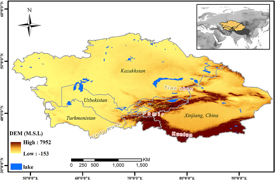
Global climate models (GCMs) are widely used to simulate the dynamics and state of the present-day climate before predicting future climate (You et al., 2010; Eyring et al., 2016), as knowledge of the ability of GCMs to simulate historical extreme precipitation events is essential for constraining climate model predictions (Allen and Ingram, 2002). Recently, state-of-the-art global climate models involved in the Coupled Model Intercomparison Project Phase 6 (CMIP6) have undergone remarkable improvements compared to previous generations, including higher resolutions and improved parameterization schemes for microphysical cloud processes and climate system biogeochemical processes compared to CMIP5 models (Eyring et al., 2016; Eyring et al., 2019), and thus better simulation capabilities are expected in the CMIP6 model to reproduce historical climate. Indeed, recent studies reported generally improved climate model performance in capturing the spatiotemporal patterns of extreme precipitation in northeastern Iran (Zamani et al., 2020), the Indian subcontinent (Gusain et al., 2020), southwestern South America (Rivera and Arnould, 2020), and East Africa (Ayugi et al., 2021). In addition, some results suggest that CMIP6 models, which generally reflect observed patterns of global and regional extreme events, show limited improvement over the CMIP5 model (Kim et al., 2020). However, most model evaluation studies focused on global or monsoon regions (e.g., You et al., 2008; Akinsanola et al., 2020; Dong and Dong, 2021; Tang et al., 2021; Vicente-Serrano et al., 2021), while efforts addressing precipitation extremes in arid and semi-arid regions are limited (Qin et al., 2021), especially in the Central Asia (hereafter CA) region (Figure 1). Guo et al. (2021) addressed the ability of CMIP6 models to simulate annual precipitation patterns and suggested that the simple ensemble mean based on all models may not be a wise choice for climate change studies in the CA region. Therefore, it is important to quantify how well each CMIP6 model simulates the variability of extreme precipitation in the CA region and to determine which CMIP6 models can be considered the most skillful models in simulating the extreme precipitation indices over the CA region based on a set of model performance metrics.

FIGURE 1

FIGURE 1. Topographic map illustrating the geographical location and overview of Central Asia.

The magnitude, frequency, and duration of precipitation extremes are typically investigated by using the extreme precipitation indices defined by the Expert Team on Climate Change Detection and Indices (ETCCDI) (Zhang et al., 2011). In previous studies, the comparison of observed and modeled extreme precipitation indices was mainly conducted by using measures such as correlation coefficients, root means square errors, percentage biases, or trend slopes of precipitation magnitude (Hu et al., 2015; Hu et al., 2019; Ayugi et al., 2021; Tang et al., 2021). However, much less attention has been paid to shape properties (related to the frequency and magnitude of extremes), such as measures of asymmetry (e.g., the skewness coefficient) and measures of tail heaviness (e.g., the kurtosis coefficient). Here, we employ a novel approach to evaluate the performance of individual models in reproducing extreme precipitation and indices, based on robust statistical measures (e.g., L-moments) and probability similarity measures (e.g., the Hellinger distance). Comparisons based on L-moments go beyond commonly used methods and help evaluate the characteristics of extreme precipitation events. Abdelmoaty et al. (2021) proposed the aforementioned approach and used it to evaluate the performance of CMIP6 models in reproducing the statistical properties of the observed annual maxima of daily precipitation worldwide and revealed that the statistical shape properties of the CMIP6 simulations agree well with the observed data. However, there is a lack of further research to support the application of this method at the regional scale, and in particular research on the mean and shape properties of extreme precipitation in arid regions, such as the region CA.

The main objective of this study was to quantitatively evaluate the performance of CMIP6 models in simulating the variance and sharp properties of present-day extreme precipitation over CA using a novel approach and various skill score metrics. The CMIP6 simulations are evaluated using three approaches: 1) one-dimensional analysis focusing on the comparison of individual L-moments of extreme precipitation over time series, 2) two-dimensional analysis focusing on the combined behavior of L-moments, and 3) probabilistic evaluation by comparing the simulated and observed distributions of extreme precipitation and indices.

2 Data and Methods

2.1 Data

Gridded observational precipitation datasets have been widely used in recent research to evaluate and assess CMIP models (Mehran et al., 2014; Booth et al., 2018). Here, we select three state-of-the-art gridded precipitation datasets from different sources as observations. The Global Precipitation Climatology Project (GPCP) blends data from rain gauge stations, satellites, and sounding observations to provide complete global precipitation estimates with 1° spatial resolution from 1996 to the present (Huffman et al., 2001). Global Precipitation Measurement Version 6 (GPM V6) is an advanced international satellite mission that provides global precipitation estimates at 0.1° resolution from June 2000 to the present (Hou et al., 2014). Bias-adjusted ERA5 reanalysis data from WATCH Forcing Data (WFDE5) provide bias-corrected precipitation derived from the European Centre for Medium-Range Weather Forecasts (ECMWF) fifth-generation atmospheric reanalysis (ERA5) at 0.5° spatial resolution and is available from 1979 to 2018 (Cucchi et al., 2020). These three gridded products were well qualified and made as homogeneous as possible (Sun et al., 2018). To maintain consistency in the assessment process, this study focused on the 2001–2014 period, which is common between CMIP6 historical simulations and observations.

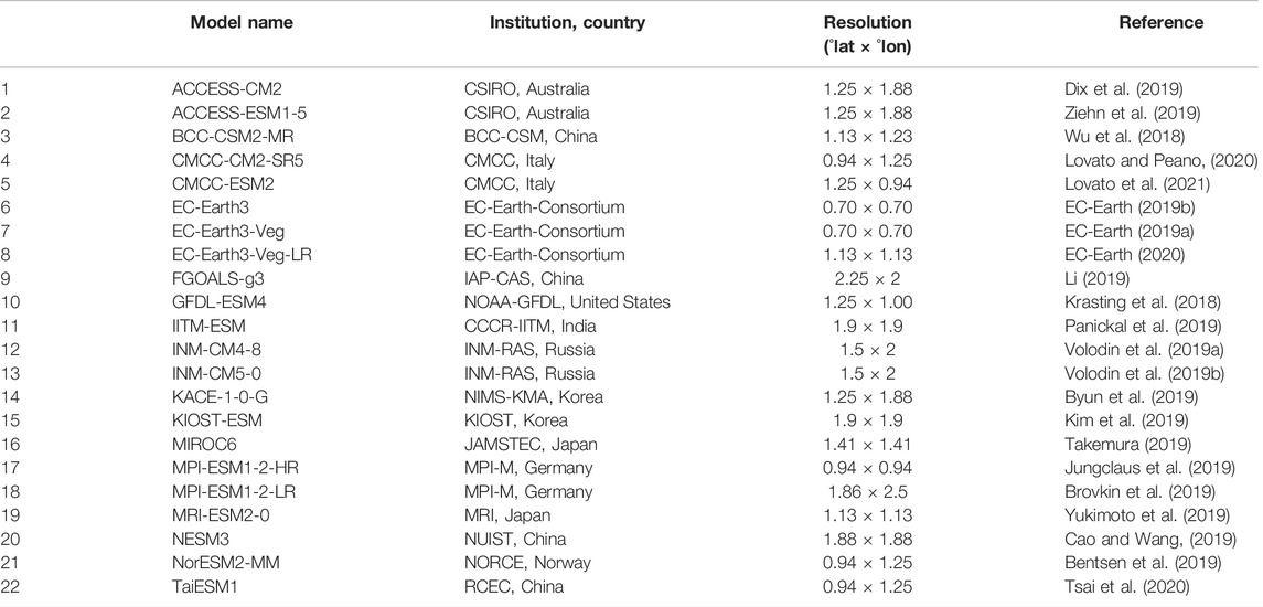
We collected the most commonly used r1i1p1f1 ensemble members from 22 CMIP6 models to evaluate their performance in simulating extreme precipitation and indices. Basic information about each model is briefly presented in Table 1, including the model name, modeling center, atmospheric resolution, and references. To facilitate the grid-to-grid comparisons between the CMIP6 model simulations and gridded observations at different resolutions (from 0.1° to 2°), we re-gridded all these data to a uniform spatial resolution (2° × 2°) using the bilinear remapping technique.

TABLE 1

TABLE 1. Information on the 22 CMIP6 global climate models used in this study.

2.2 Methods

2.2.1 Extreme Precipitation Indices

This article aims to robustly analyze the performance of CMIP6 models in characterizing historical extreme precipitation events using the indices defined in Table 2, which can detect, attribute, and project changes in extreme precipitation in multiple ways (Donat et al., 2016; Ou et al., 2013). Details on each index can be found at ETCCDI (http://etccdi.pacificclimate.org/indices_def.shtml). In early spring and late winter, heavy rains could fall on the snowpack, causing flash flooding as temperatures rise (Vionnet et al., 2020). Melting snowpack can exacerbate flooding in rivers fed by snowmelt over CA (e.g., the Syr Darya and the Amu Darya rivers) (Kure et al., 2013). In summer, increased precipitation combined with massive glacier melt at high elevations can lead to massive flooding in mountainous regions (Olsson et al., 2010). Therefore, to gain insight into the performance of the model on a seasonal scale, the analyses and calculations presented here are based on three seasons: spring (March-May, MAM), summer (June-August, JJA), and winter (December-February, DJF).

TABLE 2

TABLE 2. Definitions of the extreme precipitation indices used in the study.

2.2.2 L-Moments

We adopted new approaches following Abdelmoaty et al. (2021) to provide a comparative assessment of the ability of CMIP6 models to reproduce the spatial distribution of observed total precipitation and extreme precipitation indices. In this study, we described the difference between the observations and CMIP6 simulations with four-ordered statistics based on L-moments, including 1) mean (μ), 2) L-variation (τ₂), 3) L-skewness (τ₃), and 4) L-kurtosis (τ₄). L-moments are a set of statistics used to summarize the shape of a probability distribution, which offer numerous advantages over product moments in describing a sample or distributional characteristics (Sankarasubramanian and Srinivasan, 1999). The main advantage of L-moments over conventional moments is that L-moments are less sensitive to the effects of sampling variation and outliers in the data, allowing one to draw more reliable conclusions about the underlying probability distribution from small samples. Because of these properties, L-moments are better suited to characterize the distributional properties of highly skewed data, such as extreme precipitation events which generally exhibit moderate to strong skewness (Hosking, 1990; Hosking and Wallis, 1997).

L-moment is based on the linear combinations of probability-weighted moments (PWMs), and L signifies the linearity. PWMs defined by Greenwood et al. (1979) are given in the following:

$b_r=\frac{1}{n}{\displaystyle \sum _{j=r+1}^n\frac{(j-1)(j-2)\dots (j-r)}{(n-1)(n-1)\dots (n-r)}}{x}_j,(1)$

where $n$ = sample size and $x_j$ = jth element in ascending order.

Univariate analysis reveals the differences in L-moments between observations and simulations (Abdelmoaty et al., 2021). The first L-moment refers to the location and is known as L-mean ($l_1$). The second L-moment is a measure of scale and dispersion and termed L-scale ($l_2$). The third and fourth L-moments are measures of symmetry and peakedness, respectively. The first four L-moments have the following relevancy with PWMs:

$l_1=b_0,(2)$

$l_2=2b_1-b_0,(3)$

$l_3=6b_2-6b_1+b_0,(4)$

$l_4=20b_3-30b_2+12b_1-b_0.(5)$

The L-moment is a linear combination of the PWMs in Eqs. 2–5. L-moment ratios can be obtained by dividing the higher-order L-moments by the dispersion measure as follows:

$\mathrm{L}-\mathrm{variation}:t_2=l_2/l_1, \mathrm{where} 0\le t_2<1,(6)$

$\mathrm{L}-\mathrm{skewness}:t_3=l_3/l_2,\mathrm{where} -1\le t_3\le 1,(7)$

$\mathrm{L}-\mathrm{kurtosis}:t_4=l_4/l_2,\mathrm{where} -1\le t_4\le 1.(8)$

The ratio $l_2/l_1$ is termed the L-coefficient of variation (τ₂) and the ratio $l_3/l_2$ is referred to as L-skewness (τ₃), while the ratio $l_4/l_2$ is referred to as L-kurtosis (τ₄). Note that the relative error (%) was used to describe the difference between μ and τ₂. In contrast, the absolute error was used to describe the difference between τ₃ and τ₄ to avoid misleading large or small errors when these two values are particularly close. L-moment methods have less estimation bias than the conventional method and its asymptote are closer to a normal distribution in finite samples. However, it does not reveal whether the L-moments coincide. Therefore, we treated (u, τ₂) and (τ_2, τ₃) as bivariate variables and compared the bivariate kernel density estimation (KDE) between observations and CMIP simulations (Terrell and Scott, 1992). Finally, we estimated the Hellinger (H) distance between the observed and CMIP6 simulated bivariate L-moment densities as an overall similarity measure between densities. The H-distance is a robust technique for quantifying the similarity between two probability distributions (Hellinger, 1909). When the H-distance is 0, the two distributions are identical, and when it is 1, they are the farthest apart.

3 Results

3.1 Seasonal Precipitation and Indices

In this section, we assess the similarities and differences among the gridded observations (i.e., GPCP, GPM, and WFDE5) for precipitation spatial and frequency distributions over the CA. In spring (Figure 2) and winter (Supplementary Figure S3), all three observations show that PRCPTOT is mainly concentrated on wind-facing slopes (e.g., Tajikistan and surrounding mountains, Figure 2), as the westerlies prevail in most areas of CA (Schiemann et al., 2008), and is accompanied by the highest values of SDII, CWD, Rx5day, and R10mm and the lowest values of CDD (defined in Table 2), whereas the regions with the lowest total precipitation are mainly found in northern Xinjiang, with the highest CDD and the lowest Rx5days and R10mm. Differently, the total precipitation in summer (Supplementary Figure S2) is quite abundant on the leeward slopes of the CA mountains (e.g., eastern Tien Shan), mainly due to Tien Shan’s blocking effects which enhances subsidence over this region and essentially increases east summer precipitation (Baldwin & Vecchi, 2016). The extreme precipitation indices SDII, Rx5day, and R10mm generally follow the spatial pattern of the total precipitation while this is not the case for the CWD, indicating that the total precipitation is affected more by the intensity of precipitation events rather than the length. The ability of the CMIP6 ensemble mean to represent the spatial characteristics of total precipitation and extreme precipitation indices of observations over CA is also evaluated here. The CMIP6 ensemble means share similar spatial distributions of extreme events with all three observations on regional scales for the most part, except for CWD and R95pTOT. Although the three observations do not show significant differences in spatial distributions of the total precipitation and extreme precipitation indices at the regional scale, biases may be evident in the frequency distributions. Then, our assessment focused on comparing the area-averaged precipitation frequency distributions of the three gridded observations (GPCP, GPM, and WFDE5) and CMIP6 ensemble mean to evaluate the simulated precipitation intensity over CA from a different perspective (Supplementary Figure S1). The three observations generally agree on the distribution of precipitation frequency in spring and summer, while differences are evident in winter. The GPCP and WFDE5 exhibit higher frequency in light (<2 mm) and heavy (>10 mm) precipitation events while showing a much lower frequency in medium (2–10 mm) precipitation events compared with the GPM in winter. Furthermore, the ability of the CMIP6 ensemble means to reproduce precipitation frequency varies among the three seasons. In spring, the ensemble mean substantially underestimates (>60%) the light and middle precipitation (<10 mm), while it produces too frequently heavy precipitation (>10 mm). In winter, the ensemble mean generally matches well with the GPM, exhibiting similar bias with the other observations as in the spring, but to a lesser extent. In summer, the ensemble mean generally agrees well with the three observations, with a slight overestimation (<20%) of the light and heavy precipitation events and a slight underestimation (<23%) of the moderate precipitation events. Therefore, the differences in the precipitation frequency among the three observations are relatively small, mainly reflected in the light frequency during winter. However, this is acceptable since light rates do not generate a substantial precipitation amount over CA (Lai et al., 2020). Moreover, the pattern of the frequency distribution of GPM on the seasonal scale with the ensemble mean is much narrower compared to other observations.

FIGURE 2

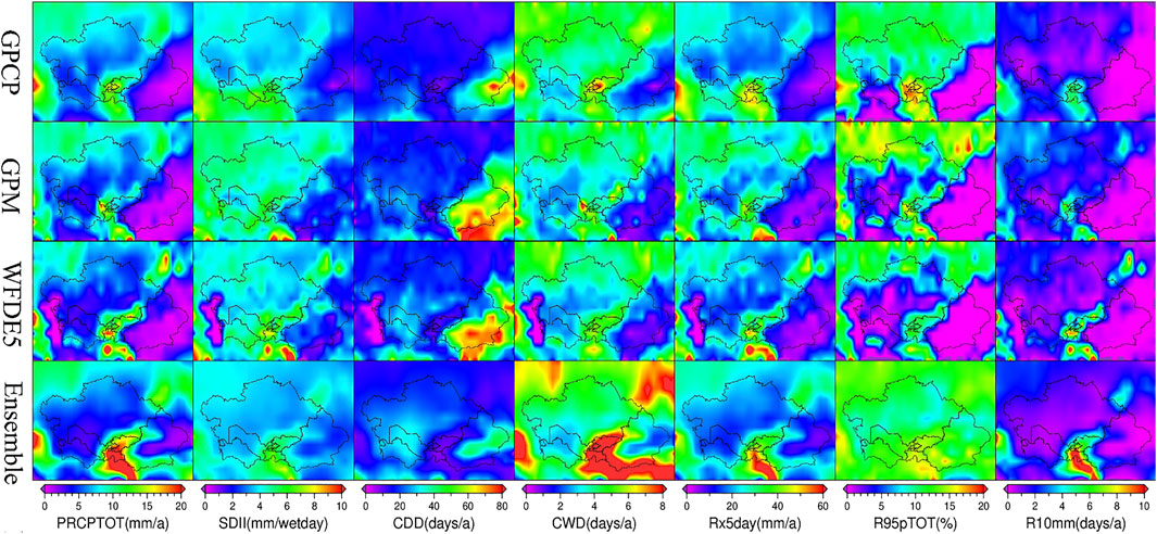
FIGURE 2. Spatial distribution of spring (MAM) total precipitation and extreme precipitation indices from three observations (GPCP, GPM, and WFDE5) and the CMIP6 multi-model ensemble mean over Central Asia for 2001–2014.

Overall, the three observations generally are consistent regarding the spatial and frequency distribution patterns of the total precipitation and extreme precipitation indices. Here, we choose GPM as the reference to evaluate the bias of the CMIP6 models. The good performance of the GPM was also reported in other studies (Sun et al., 2018; Zhang et al., 2018). For example, Zhang et al. (2018) concluded that the GPM can reproduce precipitation events incredibly well, especially light and moderate precipitation events, possibly due to the newly added Ka-band and high-frequency microwave channels.

3.2 L-Moments One-Dimensional Analysis

3.2.1 Means (μ) and Variations (τ₂)

We presented the differences in extreme precipitation indices means (μ) of CMIP6 models and GPM; none of the models can sufficiently reproduce the means of all the metrics simultaneously, with a high variability of 90% empirical confidence (Supplementary Figure S4). Fluctuations in the simulation of the mean of the total precipitation and extreme precipitation indices of CMIP6 models indicate a trade-off effect that partly explains the generally good agreement between the regional precipitation frequency from the ensemble mean and the observations (Supplementary Figure S1). In particular, these models performed relatively better at the CDD median of all extreme indices, with nearly 30%–50% of the models having a relative error within 10% over the entire period. However, the performance of the other indices is relatively poor. Most CMIP6 simulations (>65%) tend to underestimate the medians of SDII, Rx5day, and R10mm by 10%–109% for all three seasons, while they tend to overestimate CWD by 4%–109%. Seasonal differences are also observed for the same indicator. For example, an opposite trend is observed for R95PTOT in different seasons, with almost half of the models tending to overestimate R95PTOT medians in spring and winter (>15%) while tending to underestimate them in summer (>20%). Notably, an ensemble mean of the CMIP6 models only slightly constrains the mean error of most metrics and does not reduce the empirical confidence interval by 90%. This suggests that most models have consistency errors in most regions of CA.

Furthermore, the biases in the variation of the total precipitation and extreme indices as quantified by the L-moment coefficient of variation (τ₂) are investigated (Supplementary Figure S5). In general, variation (τ2) and mean (μ) behaved mostly similar in terms of changes in extreme precipitation metrics but showed some discrepancies in seasons and indices. Fluctuations in individual CMIP6 models in simulating extreme precipitation metrics are still noticeable across the seasons. Nevertheless, the CMIP6 models also perform relatively well at the CDD median among all extreme indices variations (τ2), but uncertainty increases relative to the mean (μ). SDII has more reasonable ranges of values with a general underestimate that more than 50% of the models have a relative error greater than 20% over the entire period. However, the performance of the other indices is relatively poor. Most CMIP6 simulations (>70%) tend to underestimate the variation (τ₂) medians of Rx5day, R95pTOT, and R10mm by 20%–100%, while they tend to always overestimate CWD all alone. There is a substantial difference in the ability of individual models to simulate extreme precipitation events that EC-Earth3-based models seriously overestimate the R95pTOT for both mean (μ) and variation (τ₂) while other models tend to underestimate them. Seasonal patterns were also observed. For example, variation (τ₂) of SDII, Rx5day, and R10mm median in winter are underestimated by all CMIP6 models, and 13.6% of selected models overestimate winter R95pTOT variation. The %diff of PRCPTOT in summer and CDD in spring by most models are close to zero, indicating that these models simulate the variation of summer PRCPTOT and spring CDD better than variation in another two seasons. However, an ensemble mean of the CMIP6 models performs poorly on the variation error of most metrics, with all being severely underestimated. This suggests that an ensemble mean has a problem characterizing the individual mode variations of CMIP6 over CA.

3.2.2 Skewness (τ₃) and Kurtosis (τ₄)

To investigate the shape properties of CMIP6 models in simulating extreme precipitation, we used the simple difference in analyzing skewness coefficient (τ₃) and kurtosis coefficient (τ₄). Good agreement with GPM is observed for the L-Skewness (τ₃) and L-Kurtosis (τ₄) of extreme precipitation indices (Figures 3, 4), indicating that the CMIP6 simulations reproduce the shape properties of extreme precipitation well. The median of the differences is within 10% for τ₃ and τ₄ in the vast majority of scenarios among models. In terms of τ₃ reflecting skewness, most simulations show a more skewed distribution of the PRCPTOT in summer than in spring and winter. Meanwhile, the %diff of more than half of the models is closer to zero in spring and winter, that is, these models are more accurate in simulating skewness (τ₃) in spring and winter (Figure 3). For SDII, CWD, and R95pTOT, most models simulate their skewness well in all three seasons. The %diff between the CMIP6 and GPM over the seasons is slight. Also, models simulate skewness for SDII and CWD best in spring, while models simulate skewness for R95pTOT best in summer and winter. Most models overestimate the skewness of CDD and R10mm in spring while underestimating Rx5day in the same season. In addition, most models also overestimate the skewness of CDD and R10mm in winter. However, an ensemble mean of the CMIP6 models does not improve the skewed distribution of extreme precipitation, and all metrics are slightly underestimated. This is similar to the percentage difference in extreme precipitation indices variation and suggests that an ensemble mean is difficult in characterizing the individual mode variations of CMIP6 over CA.

FIGURE 3

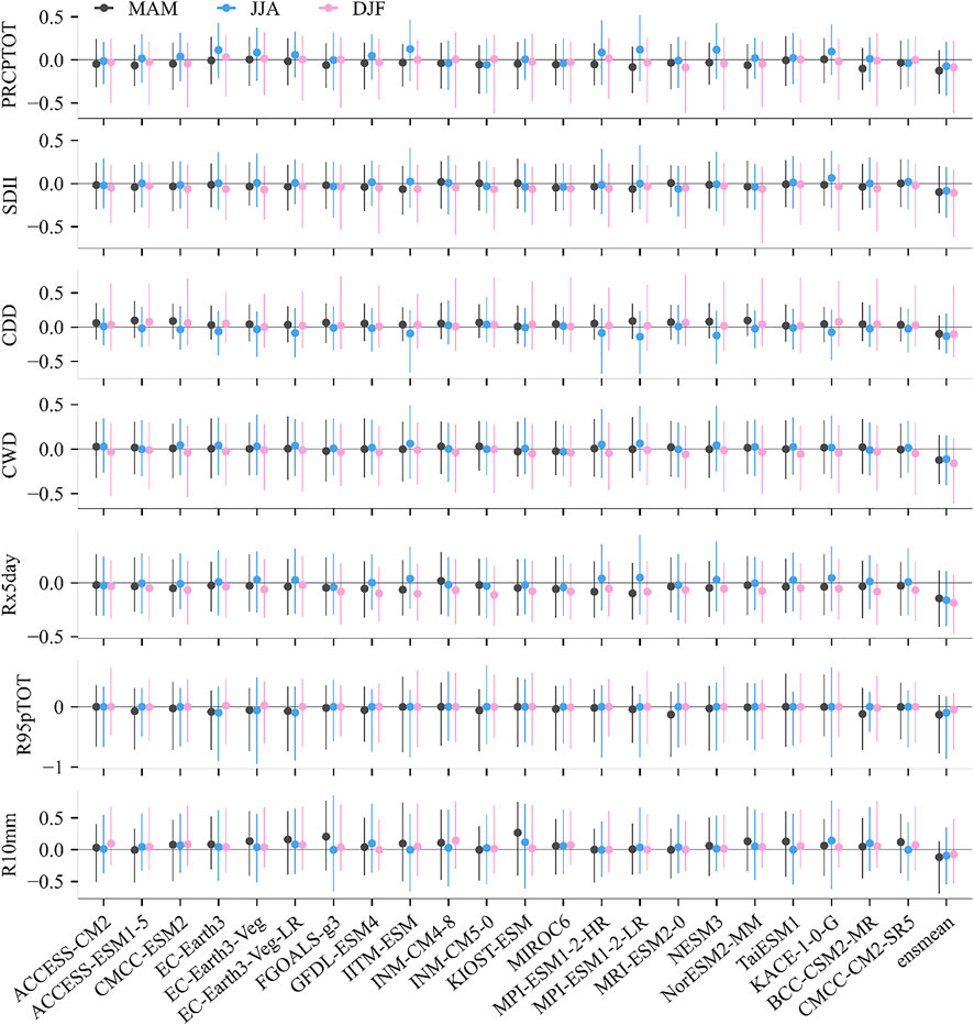
FIGURE 3. Percentage difference in L-skewness (τ₃) of total precipitation and extreme precipitation indices between the GPM and CMIP6 models (including the multi-model ensemble mean) in spring (MAM), summer (JJA), and winter (DJF). The total precipitation and SDII, CDD, CWD, Rx5day, R95pTOT, and R10mm are shown from top to bottom. The point represents the median, and the error bar indicates the 90% empirical confidence interval. The triangle in the graph indicates a bias greater than 150%.

FIGURE 4

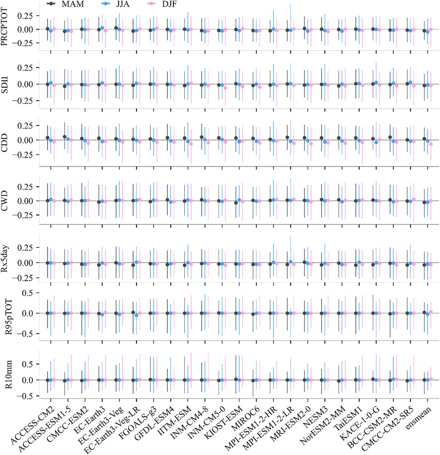
FIGURE 4. Percentage difference in L-kurtosis (τ₄) of total precipitation and extreme precipitation indices between the GPM and CMIP6 models (including the multi-model ensemble mean) in spring (MAM), summer (JJA), and winter (DJF). The total precipitation and SDII, CDD, CWD, Rx5day, R95pTOT, and R10mm are shown from top to bottom. The point represents the median, and the error bar indicates the 90% empirical confidence interval. The triangle in the graph indicates a bias greater than 150%.

In all seasons, the shape feature kurtosis (τ₄) of the simulations for total precipitation and extreme precipitation indices is close to the observations (Figure 4), and the medians of PRCPTOT, SDII, CWD, R95pTOT, and R10mm perform well. The kurtosis for the Rx5day median of most model simulations is slightly underestimated in each season. The kurtosis of the simulation of CDD in summer is closest to the observation, while the kurtosis of the simulation in spring and winter overestimates and underestimates the observation, respectively. From the comparison of the two shape features (τ₃ and τ₄), the simulations of all indices of kurtosis of the CMIP6 model are generally better than those of skewness, e.g., %diff is closer to zero for τ₄ (Figures 3, 4). Meanwhile, an ensemble mean of the CMIP6 models only slightly constrains the kurtosis error of most metrics and does not reduce the %diff of the median.

3.3 L-Moment Two-Dimensional Analysis

Comparing the separate behavior of each L-moment can be helpful, yet it is more robust and comprehensive to compare a wider scale of the total precipitation and extreme indices behaviors. First, we used non-parametric kernel bivariate densities to describe the simultaneous behaviors of the total precipitation and extreme indices L-moments to assess CMIP6 simulations. EC-EARTH3 is the best-performed model, according to the kernel bivariate density analysis, and then we choose EC-EARTH3 for the detailed description, others see supplementary (Supplementary Figures S6–47). The density distributions (the blue area in Figures 5, 6) for GPM and EC-Earth3 were calculated and compared with the simulations. Bivariate densities show high variability between models for the mean (μ) and variation (τ₂) pairs, and in most cases do not match observations from GPM (examples are shown in Figure 5), including SDII, CWD, and Rx5day, especially for the intensity of extreme precipitation indices R95pTOT and R10mm. In contrast, total precipitation performed relatively well in the density distributions between simulations and GPM observations. Seasonality, SDII, and CWD in summer and CWD and Rx5day in spring also show high mismatching for μ and τ₂ pair between simulation and observation, indicating high variability among CMIP6 simulations. Then, the highest probability region (HPR, red cross in Figures 5, 6) for GPM was calculated and compared with simulations. In summer, the (μ, τ₂) peaks generated from CMIP6 simulations match with observations (Figure 5B). In contrast, the peak points of simulations differ from the observational peaks in spring and winter (Figures 5A,C). For example, there are some differences between the observations and simulations of R95pTOT, SDII, and Rx5day for highest probability regions (HPR), which means that the model has a poor simulation effect on these indices on the bivariate distribution of (μ, τ₂). Although there exists the good matching in μ and τ₂ for total precipitation individually (Figures 3, 4), simultaneous behavior mismatches.

FIGURE 5

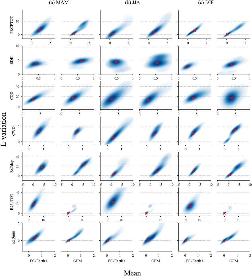
FIGURE 5. Kernel bivariate densities for a simulation of EC-Earth3 and GPM with the highest probable region of mean and L-variation densities in (A) spring (MAM), (B) summer (JJA), and (C) winter (DJF). The red cross represents the highest probability region.

FIGURE 6

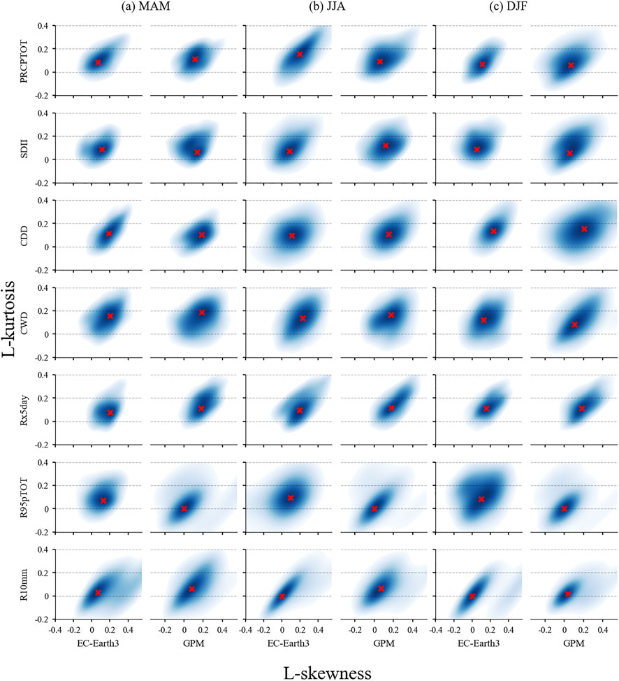
FIGURE 6. Kernel bivariate densities for a simulation of EC-Earth3 and GPM with the highest probable region of L-skewness and L-kurtosis densities in (A) spring (MAM), (B) summer (JJA), and (C) winter (DJF).The red cross represents the highest probability region.

Second, unlike the striped distribution of the (μ, τ₂) kernel bivariate density, the distribution of the higher order L-moments (τ₃, τ₄) in Figure 6 tends to be round. Bivariate densities for (τ₃, τ₄) generated from the CMIP6 simulations agree with observations for most indices in all seasons, especially for total precipitation. However, the bivariate densities of R95pTOT show high variability between simulations and GPM observations. For (τ₃, τ₄), Figure 6 exhibits a good agreement of the peak points of HPR between simulations and GPM observations for most cases, including PRCPTOT in winter, CDD in spring and summer, and CWD in spring. Among all extreme precipitation indices, R95pTOT shows more different shape features between simulations and observations in all seasons. Therefore, the results reveal a matching in the shape properties of total precipitation and extreme precipitation indices, with simultaneous behavior of the higher order L-moments (τ₃, τ₄) matches.

Third, the Hellinger distance (H) is used to calculate the overall difference between bivariate densities of CMIP6 models simulations and GPM (Figures 7, 8). H distances for the mean (μ) and L-variation (τ₂) are calculated for each model (Figure 7). For mean (μ) and L-variation (τ₂) densities of total precipitation, all CMIP6 models have H >0.3, with EC-Earth3 having the smallest H (0.35). For most models, H distances of R95pTOT and R10mm are higher than other indices which can reach up to 0.6–0.8, showing that the simulating performance in winter is poor for the two indices. The H distance of R95pTOT is quite special which obtained by each model varies greatly, and CMCC-ESM2 and TaiESMI perform best in all three seasons for R95pTOT. For CDD and R95pTOT, the H distance of most results shows that H distance in summer is lower than in spring and winter. H distance in summer for Rx5day of more than half models is higher than in spring and winter. For CWD and Rx5day, the higher summer H distance indicates that the IITM-ESM model is poor at simulating observations in summer. In terms of H distance in spring, EC-Earth-based models show the lowest value among CMIP6 models on PRCPTOT, CDD, and CWD.

FIGURE 7

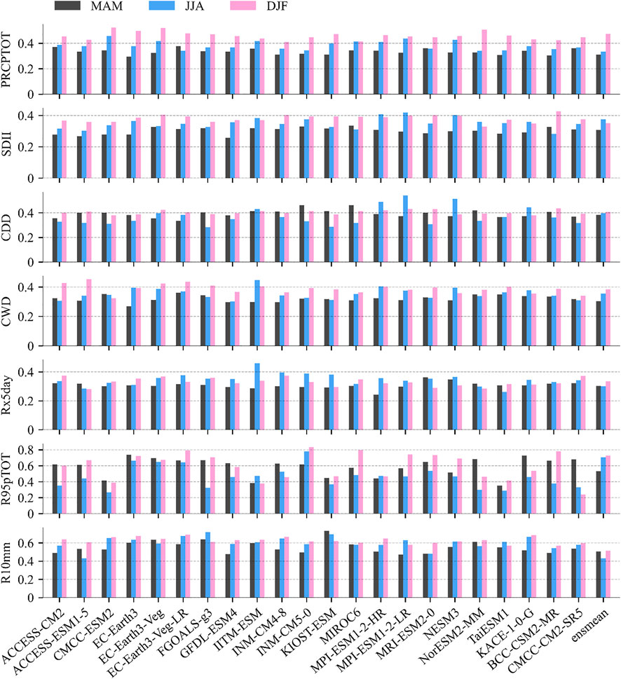
FIGURE 7. Hellinger distance in mean and L-variation between the bivariate empirical densities of CMIP6 models and the GPM.

FIGURE 8

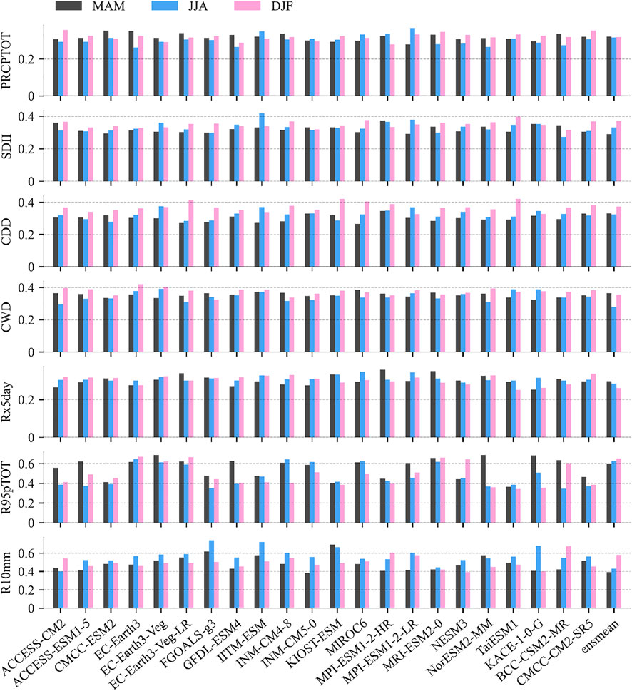
FIGURE 8. Hellinger distance in L-skewness and L-kurtosis between bivariate empirical densities of CMIP6 models and the GPM.

For L-skewness (τ₃) and L-kurtosis (τ₄) densities of total precipitation and indices, most CMIP6 models have H < 0.35 (Figure 8). The H distances of τ₃ and τ₄ bivariate densities for PRCPTOT and Rx5day are the lowest (H < 0.3) among indices, while H distances for R95pTOT and R10mm are the highest. CMIP6 models can simulate well the shape characteristics of PRCPTOT, CWD, and R10mm in summer but have difficulty in simulating the shape characteristics well of CDD in winter and R95pTOT in spring.

On the whole, there are significant differences between the performance between H distance of τ₃ and τ₄ bivariate densities (shape characteristics) and μ and τ₂ densities (mean and variation characteristics). The result shows that a good representation of higher-order L-moments’ joint behavior can be found in L-skewness (τ₃) and L-kurtosis (τ₄) densities rather than mean (μ) and L-variation (τ₂).

4 Discussion

Although global climate models have improved in the recent decade (Kim et al., 2020; Ayugi et al., 2021), it seems not to appear to be the case for arid and semi-arid regions such as CA (Mehran et al., 2014; Guo et al., 2021; Qin et al., 2021). The uncertainties for CMIP6 in assessing precipitation extremes arise from our limited knowledge of the key physical processes for circulation changes. For example, the increase in precipitation would be accompanied by the increase in water vapor but offset by the weakened circulation (Chen et al., 2020). CMIP models generally overestimate total precipitation in regions with steep topography (Mehran et al., 2014; Ji et al., 2015). The topographic correction could improve the performance of gridded precipitation. However, the effect of topography has not been fully considered in CMIP6 models due to their coarse resolution (Eyring et al., 2016). Meanwhile, even when a higher resolution model is used, the difference between observed and simulated precipitation can be large and strongly dependent on the methods (Freychet et al., 2016). A group of CMIP model simulations typically have large differences that can vary widely (Dong and Dong, 2021; Tang et al., 2021). It is the case for our study that most of the evaluations show good performance, but the results of individual models vary. Although an ensemble mean of 22 models is used in our study to evaluate the extreme precipitation results to reduce uncertainty, it appears that significant information is lost for some indices and features (Supplementary Figure S5). This study supported the view of Abdelmoaty et al. (2021) and concluded that CMIP6 simulations reproduce shape properties of the extreme precipitation index distributions better than the mean and the variability. Interestingly, the simultaneous behavior of higher order L-moments (τ₃ and τ₄) generated from the model simulations performed better on a global scale than in the CA region. Moreover, the scatter due to seasonal variability is comparable to the scatter among the 22 CMIP6 models, indicating the remarkable influence of seasonal variability on the simulations. Further efforts should be devoted to seasonal climate simulations, which can improve the simulation of precipitation extremes.

Previous analysis of CMIP models evaluated the mean and variance but not the shape properties of the climate variables. Since skewness is suitable for assessing asymmetry and kurtosis is suitable for assessing volatility and uncertainty, higher moment assumptions associated with higher-order central moments should be explored more than univariate L-moments to play a more central role in the assessment (Serfling and Xiao, 2007). The popularity of the L-moments method is due to its robustness to outliers in the data (El-Magd, 2010), but the L-moments method is not very efficient for predicting events with large return periods (Zakaria et al., 2012). Zakaria et al. (2012) believe that direct visual inspection of the L-moment diagram (skewness and kurtosis) is subjective, which may also be an aspect of the uncertainty of the L-moment method. However, in our study, we introduce %diff to make the comparison quite objective. To improve the evaluation ability and applicability, researchers improved trimmed L-moment methods and partial L-moment methods based on L-moment (Elamir and Seheult, 2003). In the future, TL-moment and PL-moment methods could be used in our follow-up work for comparison with current methods or other aspects of assessment.

5 Conclusion

In this work, we quantitatively evaluated the performance of 22 CMIP6 models in simulating total precipitation and extreme precipitation indices over CA on a seasonal scale for the period 2001–2014 using quality-controlled gridded observations (GPCP, GPM, and WFDE5), and the benchmark set is GPM. The study evaluated the performance of CMIP6 models using novel methodologies to assess biases not only in mean and variation but also in higher-order L-moments and bivariate properties, including 1) summary statistics as expressed by univariate analysis of L-moments and 2) the bivariate kernel densities of (mean, L-variation) and (L-skewness, L-kurtosis) by applying HPR and using Hellinger distance as a measure of agreement. We have highlighted the mean and sharp properties of the distributions of CMIP6 models that perform well or poorly. Fluctuations in the simulation of extreme precipitation indicators across CMIP6 models are also evident among seasons. The main findings of this study can be summarized as follows:

1) CMIP6 simulations reproduce the shape properties skewness (τ₃) and kurtosis (τ₄) of the distributions of precipitation extremes better than the mean (μ) and variability (τ₂) over CA. An ensemble mean of the CMIP6 models does not improve the performance of the variation and skewness of the simulated precipitation extremes, while it only slightly constrains the mean and kurtosis error of most metrics.

2) There are simultaneous behavior mismatches in L-moments (μ and τ₂) of the bivariate densities, while the higher order L-moments (τ₃ and τ₄) generated from the model simulations match with observations, suggesting that the CMIP6 simulations can better reproduce the shape properties of the precipitation extremes than their mean and variance.

3) Among all assessment models, EC-Earth3 appears to perform very well in all systematic assessment methods, with a small percentage difference in total precipitation means (∼15%) and low Hellinger distance (H = 0.38) for mean and bivariate density.

This study lays the foundation for improving the performance of sharp properties of extreme precipitation events over CA.

Data Availability Statement

The raw data supporting the conclusion of this article will be made available by the authors, without undue reservation.

Author Contributions

ZL contributed to the conception and design of the study. GZ, JD, and XX performed the statistical analysis. ZL and JD wrote the first draft of the manuscript and sections of the manuscript. All authors contributed to manuscript revision and read and approved the submitted version.

Funding

This study was financially supported by the National Natural Science Foundation of China (Grant No. 41871020), the National Key Research and Development Program of China (2020YFB1600103), and the National Natural Science Foundation of China (Grant No.42101130).

Conflict of Interest

The authors declare that the research was conducted in the absence of any commercial or financial relationships that could be construed as a potential conflict of interest.

Publisher’s Note

All claims expressed in this article are solely those of the authors and do not necessarily represent those of their affiliated organizations, or those of the publisher, the editors, and the reviewers. Any product that may be evaluated in this article, or claim that may be made by its manufacturer, is not guaranteed or endorsed by the publisher.

Supplementary Material

The Supplementary Material for this article can be found online at: https://www.frontiersin.org/articles/10.3389/feart.2022.918337/full#supplementary-material

References

Abdelmoaty, H. M., Papalexiou, S. M., Rajulapati, C. R., and AghaKouchak, A. (2021). Biases Beyond the Mean in CMIP6 Extreme Precipitation: A Global Investigation. Earth's Future 9(10), e2021ef002196. doi:10.1029/2021ef002196

CrossRef Full Text | Google Scholar

Abu El-Magd, N. A. T. (2010). TL-moments of the Exponentiated Generalized Extreme Value Distribution. J. Adv. Res. 1(4), 351–359. doi:10.1016/j.jare.2010.06.003

CrossRef Full Text | Google Scholar

Akinsanola, A. A., Kooperman, G. J., Reed, K. A., Pendergrass, A. G., and Hannah, W. M. (2020). Projected Changes in Seasonal Precipitation Extremes over the United States in CMIP6 Simulations. Environ. Res. Lett. 15(10), 104078. doi:10.1088/1748-9326/abb397

CrossRef Full Text | Google Scholar

Allen, M. R., and Ingram, W. J. (2002). Constraints on Future Changes in Climate and the Hydrologic Cycle. Nature 419(6903), 228–232. doi:10.1038/nature01092

PubMed Abstract | CrossRef Full Text | Google Scholar

Ayugi, B., Zhihong, J., Zhu, H., Ngoma, H., and Dike, V. (2021). Comparison of CMIP6 and CMIP5 Models in Simulating Mean and Extreme Precipitation over East Africa. Int. J. Climatol. 41, 6474–6496. doi:10.1002/joc.7207

CrossRef Full Text | Google Scholar

Baldwin, J., and Vecchi, G. (2016). Influence of the Tian Shan on Arid Extratropical Asia. J. Clim. 29(16), 5741–5762. doi:10.1175/jcli-d-15-0490.1

CrossRef Full Text | Google Scholar

Bentsen, M., Oliviè, D. J. L., Seland, Ø., Toniazzo, T., Gjermundsen, A., Graff, L. S., et al. (2019). NCC NorESM2-MM Model Output Prepared for CMIP6 CMIP. Oslo, Norway: Earth System Grid Federation. doi:10.22033/ESGF/CMIP6.506

CrossRef Full Text | Google Scholar

Booth, J. F., Naud, C. M., and Willison, J. (2018). Evaluation of Extratropical Cyclone Precipitation in the North Atlantic Basin: An Analysis of ERA-Interim, WRF, and Two CMIP5 Models. J. Clim. 31(6), 2345–2360. doi:10.1175/jcli-d-17-0308.1

PubMed Abstract | CrossRef Full Text | Google Scholar

Brovkin, V., Wieners, K-H., Giorgetta, M., Jungclaus, J., Reick, C., Esch, M., et al. (2019). MPI-M MPIESM1.2-LR Model Output Prepared for CMIP6 C4MIP. Hamburg, Germany: Earth System Grid Federation. doi:10.22033/ESGF/CMIP6.748

CrossRef Full Text | Google Scholar

Byun, Y.-H., Lim, Y-J., Sung, H. M., Kim, J., Sun, M., Kim, B-H., et al. (2019). NIMS-KMA KACE1.0-G Model Output Prepared for CMIP6 CMIP. Jejudo, Republic of Korea: Earth System Grid Federation. doi:10.22033/ESGF/CMIP6.2241

CrossRef Full Text | Google Scholar

Cao, J., and Wang, B. (2019). NUIST NESMv3 Model Output Prepared for CMIP6 CMIP. Nanjing, China: Earth System Grid Federation. doi:10.22033/ESGF/CMIP6.2021

CrossRef Full Text | Google Scholar

Chen, Z., Zhou, T., Zhang, L., Chen, X., Zhang, W., and Jiang, J. (2020). Global Land Monsoon Precipitation Changes in CMIP6 Projections. Geophys. Res. Lett. 47 (14), e86902. doi:10.1029/2019gl086902

CrossRef Full Text | Google Scholar

Cucchi, M., Weedon, G. P., Amici, A., Bellouin, N., Lange, S., Müller Schmied, H., et al. (2020). WFDE5: Bias-Adjusted ERA5 Reanalysis Data for Impact Studies. Earth Syst. Sci. Data 12 (3), 2097–2120. doi:10.5194/essd-12-2097-2020

CrossRef Full Text | Google Scholar

Dix, M., Bi, D., Dobrohotoff, P., Fiedler, R., Harman, I., Law, R., et al. (2019). CSIRO-ARCCSS ACCESS-CM2 Model Output Prepared for CMIP6 CMIP. Victoria, Australia: Earth System Grid Federation. doi:10.22033/ESGF/CMIP6.2281

CrossRef Full Text | Google Scholar

Donat, M. G., Lowry, A. L., Alexander, L. V., O’Gorman, P. A., and Maher, N. (2016). More Extreme Precipitation in the World's Dry and Wet Regions. Nat. Clim. Change 6(5), 508–513. doi:10.1038/nclimate2941

CrossRef Full Text | Google Scholar

Dong, T., and Dong, W. (2021). Evaluation of Extreme Precipitation over Asia in CMIP6 Models. Clim. Dyn. 57(7-8), 1751–1769. doi:10.1007/s00382-021-05773-1

CrossRef Full Text | Google Scholar

Doocy, S., Daniels, A., Murray, S., and Kirsch, T. D. (2013). The Human Impact of Floods: a Historical Review of Events 1980-2009 and Systematic Literature Review. PLoS Curr. 5, ecurrents.dis.f4deb457904936b07c09daa98ee8171a. doi:10.1371/currents.dis.f4deb457904936b07c09daa98ee8171a:

PubMed Abstract | CrossRef Full Text | Google Scholar

EC-Earth (2019b). EC-Earth-Consortium EC-Earth3 Model Output Prepared for CMIP6 CMIP Historical. Norrkoping, Sweden: Earth System Grid Federation. doi:10.22033/ESGF/CMIP6.4700

CrossRef Full Text | Google Scholar

EC-Earth (2019a). EC-Earth-Consortium EC-Earth3-Veg Model Output Prepared for CMIP6 ScenarioMIP. Norrkoping, Sweden: Earth System Grid Federation. doi:10.22033/ESGF/CMIP6.727

CrossRef Full Text | Google Scholar

EC-Earth (2020). EC-Earth-Consortium EC-Earth3-Veg-LR Model Output Prepared for CMIP6 CMIP Historical. Norrkoping, Sweden: Earth System Grid Federation. doi:10.22033/ESGF/CMIP6.4707

CrossRef Full Text | Google Scholar

Elamir, E. A. H., and Seheult, A. H. (2003). Trimmed L-Moments. Comput. Statistics Data Analysis 43(3), 299–314. doi:10.1016/s0167-9473(02)00250-5

CrossRef Full Text | Google Scholar

Eyring, V., Bony, S., Meehl, G. A., Senior, C. A., Stevens, B., Stouffer, R. J., et al. (2016). Overview of the Coupled Model Intercomparison Project Phase 6 (CMIP6) Experimental Design and Organization. Geosci. Model Dev. 9(5), 1937–1958. doi:10.5194/gmd-9-1937-2016

CrossRef Full Text | Google Scholar

Eyring, V., Cox, P. M., Flato, G. M., Gleckler, P. J., Abramowitz, G., Caldwell, P., et al. (2019). Taking Climate Model Evaluation to the Next Level. Nat. Clim. Change 9 (2), 102–110. doi:10.1038/s41558-018-0355-y

CrossRef Full Text | Google Scholar

Freychet, N., Duchez, A., Wu, C.-H., Chen, C.-A., Hsu, H.-H., Hirschi, J., et al. (2016). Variability of Hydrological Extreme Events in East Asia and Their Dynamical Control: a Comparison between Observations and Two High-Resolution Global Climate Models. Clim. Dyn. 48 (3-4), 745–766. doi:10.1007/s00382-016-3108-5

CrossRef Full Text | Google Scholar

Greenwood, J. A., Landwehr, J. M., Matalas, N. C., and Wallis, J. R. (1979). Probability Weighted Moments: Definition and Relation to Parameters of Several Distributions Expressable in Inverse Form. Water Resour. Res. 15 (5), 1049–1054.

CrossRef Full Text | Google Scholar

Guo, H., Bao, A., Chen, T., Zheng, G., Wang, Y., Jiang, L., et al. (2021). Assessment of CMIP6 in Simulating Precipitation over Arid Central Asia. Atmos. Res. 252, 105451. doi:10.1016/j.atmosres.2021.105451

CrossRef Full Text | Google Scholar

Gusain, A., Ghosh, S., and Karmakar, S. (2020). Added Value of CMIP6 over CMIP5 Models in Simulating Indian Summer Monsoon Rainfall. Atmos. Res. 232, 104680. doi:10.1016/j.atmosres.2019.104680

CrossRef Full Text | Google Scholar

Hellinger, E. (1909). Neue Begründung der Theorie quadratischer Formen von unendlichvielen Veränderlichen. J. für die reine und angewandte Math. 1909(136), 210–271. doi:10.1515/crll.1909.136.210

CrossRef Full Text | Google Scholar

Hosking, J. R. M. (1990). L-Moments: Analysis and Estimation of Distributions Using Linear Combinations of Order Statistics. J. R. Stat. Soc. Ser. B Methodol. 52(1), 105–124. doi:10.1111/j.2517-6161.1990.tb01775.x

CrossRef Full Text | Google Scholar

Hosking, J. R. M., and Wallis, J. R. (1997). Regional Frequency Analysis. Cambridge: Cambridge University Press.

Google Scholar

Hou, A. Y., Kakar, R. K., Neeck, S., Azarbarzin, A. A., Kummerow, C. D., Kojima, M., et al. (2014). The Global Precipitation Measurement Mission. Bull. Amer. Meteor. Soc. 95(5), 701–722. doi:10.1175/bams-d-13-00164.1

CrossRef Full Text | Google Scholar

Hu, Z., Chen, X., Chen, D., Li, J., Wang, S., Zhou, Q., et al. (2019). “Dry Gets Drier, Wet Gets Wetter”: A Case Study over the Arid Regions of Central Asia. Int. J. Climatol. 39(2), 1072–1091. doi:10.1002/joc.5863

CrossRef Full Text | Google Scholar

Hu, Z., Li, Q., Chen, X., Teng, Z., Chen, C., Yin, G., et al. (2015). Climate Changes in Temperature and Precipitation Extremes in an Alpine Grassland of Central Asia. Theor. Appl. Climatol. 126(3-4), 519–531. doi:10.1007/s00704-015-1568-x

CrossRef Full Text | Google Scholar

Huffman, G. J., Adler, R. F., Morrissey, M. M., Bolvin, D. T., Curtis, S., Joyce, R., et al. (2001). Global Precipitation at One-Degree Daily Resolution from Multisatellite Observations. J. Hydrometeor 2(1), 36–50. doi:10.1175/1525-7541(2001)002<0036:gpaodd>2.0.co;2

CrossRef Full Text | Google Scholar

IPCC (2014). Climate Change 2014: Synthesis Report. Contribution of Working Groups I, II and III to the Fifth Assessment Report of the Intergovernmental Panel on Climate Change. Switzerland: IPCC.

Google Scholar

Ji, M., Huang, J., Xie, Y., and Liu, J. (2015). Comparison of Dryland Climate Change in Observations and CMIP5 Simulations. Adv. Atmos. Sci. 32(11), 1565–1574. doi:10.1007/s00376-015-4267-8

CrossRef Full Text | Google Scholar

Jungclaus, J., Bittner, M., Wieners, K-H., Wachsmann, F., Schupfner, M., Legutke, S., et al. (2019). MPI-M MPIESM1.2-HR Model Output Prepared for CMIP6 CMIP. Hamburg, Germany: Earth System Grid Federation. doi:10.22033/ESGF/CMIP6.741

CrossRef Full Text | Google Scholar

Kim, Y.-H., Min, S.-K., Zhang, X., Sillmann, J., and Sandstad, M. (2020). Evaluation of the CMIP6 Multi-Model Ensemble for Climate Extreme Indices. Weather Clim. Extrem. 29, 100269. doi:10.1016/j.wace.2020.100269

CrossRef Full Text | Google Scholar

Kim, Y., Noh, Y., Kim, D., Lee, M-I., Lee, H. J., Kim, S. Y., et al. (2019). KIOST KIOST-ESM Model Output Prepared for CMIP6 CMIP. Busan, Republic of Korea: Earth System Grid Federation. doi:10.22033/ESGF/CMIP6.1922

CrossRef Full Text | Google Scholar

Krasting, J. P., John, J. G., Blanton, C., McHugh, C., Nikonov, S., Radhakrishnan, A., et al. (2018). Noaa-gfdl Gfdl-Esm4 Model Output Prepared for Cmip6 Cmip Historical. Princeton, USA: Earth System Grid Federation. doi:10.22033/ESGF/CMIP6.8597

CrossRef Full Text | Google Scholar

Kure, S., Jang, S., Ohara, N., Kavvas, M. L., and Chen, Z. Q. (2013). Hydrologic Impact of Regional Climate Change for the Snowfed and Glacierfed River Basins in the Republic of Tajikistan: Hydrological Response of Flow to Climate Change. Hydrol. Process. 27(26), 4057–4070. doi:10.1002/hyp.9535

CrossRef Full Text | Google Scholar

Lai, S., Xie, Z., Bueh, C., and Gong, Y. (2020). Fidelity of the APHRODITE Dataset in Representing Extreme Precipitation over Central Asia. Adv. Atmos. Sci. 37(12), 1405–1416. doi:10.1007/s00376-020-0098-3

CrossRef Full Text | Google Scholar

Li, L. (2019). CAS FGOALS-G3 Model Output Prepared for CMIP6 CMIP 1pctCO2. Beijing, China: Earth System Grid Federation. doi:10.22033/ESGF/CMIP6.3055

CrossRef Full Text | Google Scholar

Lovato, T., Peano, D., and Butenschön, M. (2021). CMCC CMCC-ESM2 Model Output Prepared for CMIP6 C4MIP 1pctCO2-Bgc. Lecce, Italy: Earth System Grid Federation. doi:10.22033/ESGF/CMIP6.13170

CrossRef Full Text | Google Scholar

Lovato, T., and Peano, D. (2020). CMCC CMCC-CM2-SR5 Model Output Prepared for CMIP6 CMIP 1pctCO2. Lecce, Italy: Earth System Grid Federation. doi:10.22033/ESGF/CMIP6.3721

CrossRef Full Text | Google Scholar

Mehran, A., AghaKouchak, A., and Phillips, T. J. (2014). Evaluation of CMIP5 Continental Precipitation Simulations Relative to Satellite-Based Gauge-Adjusted Observations. J. Geophys. Res. Atmos. 119(4), 1695–1707. doi:10.1002/2013jd021152

CrossRef Full Text | Google Scholar

Olsson, O., Gassmann, M., Wegerich, K., and Bauer, M. (2010). Identification of the Effective Water Availability from Streamflows in the Zerafshan River Basin, Central Asia. J. Hydrology 390(3-4), 190–197. doi:10.1016/j.jhydrol.2010.06.042

CrossRef Full Text | Google Scholar

Ou, T., Chen, D., Linderholm, H. W., and Jeong, J.-H. (2013). Evaluation of Global Climate Models in Simulating Extreme Precipitation in China. Tellus A Dyn. Meteorology Oceanogr. 65(1), 19799. doi:10.3402/tellusa.v65i0.19799

CrossRef Full Text | Google Scholar

Panickal, S., Raghavan, K., Gopinathan, P. A., Narayanasetti, S., Choudhury, A. D., Singh, M., et al. (2019). CCCR-IITM IITM-ESM Model Output Data Prepared for CMIP6 CMIP/DECK. Maharashtra, India: Earth System Grid Federation. doi:10.22033/ESGF/CMIP6.44

CrossRef Full Text | Google Scholar

Qin, J., Su, B., Tao, H., Wang, Y., Huang, J., and Jiang, T. (2021). Projection of Temperature and Precipitation under SSPs-RCPs Scenarios over Northwest China. Front. Earth Sci. 15(1), 23–37. doi:10.1007/s11707-020-0847-8

CrossRef Full Text | Google Scholar

Rivera, J. A., and Arnould, G. (2020). Evaluation of the Ability of CMIP6 Models to Simulate Precipitation over Southwestern South America: Climatic Features and Long-Term Trends (1901-2014). Atmos. Res. 241, 104953. doi:10.1016/j.atmosres.2020.104953

CrossRef Full Text | Google Scholar

Sankarasubramanian, A., and Srinivasan, K. (1999). Investigation and Comparison of Sampling Properties of L-Moments and Conventional Moments. J. Hydrology 218(1), 13–34. doi:10.1016/S0022-1694(99)00018-9

CrossRef Full Text | Google Scholar

Schiemann, R., Lüthi, D., Vidale, P. L., and Schär, C. (2008). The Precipitation Climate of Central Asia-Intercomparison of Observational and Numerical Data Sources in a Remote Semiarid Region. Int. J. Climatol. 28(3), 295–314. doi:10.1002/joc.1532

CrossRef Full Text | Google Scholar

Serfling, R., and Xiao, P. (2007). A Contribution to Multivariate L-Moments: L-Comoment Matrices. J. Multivar. Analysis 98(9), 1765–1781. doi:10.1016/j.jmva.2007.01.008

CrossRef Full Text | Google Scholar

Sun, Q., Miao, C., Duan, Q., Ashouri, H., Sorooshian, S., and Hsu, K. L. (2018). A Review of Global Precipitation Data Sets: Data Sources, Estimation, and Intercomparisons. Rev. Geophys. 56(1), 79–107. doi:10.1002/2017rg000574

CrossRef Full Text | Google Scholar

Takemura, T. (2019). MIROC MIROC6 Model Output Prepared for CMIP6 AerChemMIP. Hyogo, Japan: Earth System Grid Federation. doi:10.22033/ESGF/CMIP6.9121

CrossRef Full Text | Google Scholar

Tang, B., Hu, W., and Duan, A. (2021). Assessment of Extreme Precipitation Indices over Indochina and South China in CMIP6 Models. J. Clim. 34 (18), 7507–7524. doi:10.1175/jcli-d-20-0948.1

CrossRef Full Text | Google Scholar

Terrell, G. R., and Scott, D. W. (1992). Variable Kernel Density Estimation. Ann. Statistics, 1236–1265. doi:10.1214/aos/1176348768

CrossRef Full Text | Google Scholar

Trenberth, K. E., Dai, A., Rasmussen, R. M., and Parsons, D. B. (2003). The Changing Character of Precipitation. Bull. Am. Meteorological Soc. 84(9), 1205–1218. doi:10.1175/bams-84-9-1205

CrossRef Full Text | Google Scholar

Tsai, I. C., Lee, W.-L., and Hsu, H.-H. (2020). AS-RCEC TaiESM1.0 Model Output Prepared for CMIP6 AerChemMIP. Taiwan, China: Earth System Grid Federation. doi:10.22033/ESGF/CMIP6.9682

CrossRef Full Text | Google Scholar

Utsumi, N., Seto, S., Kanae, S., Maeda, E. E., and Oki, T. (2011). Does Higher Surface Temperature Intensify Extreme Precipitation? Geophys. Res. Lett. 38(16), 708–713. doi:10.1029/2011gl048426

CrossRef Full Text | Google Scholar

Vicente-Serrano, S. M., García-Herrera, R., Peña-Angulo, D., Tomas-Burguera, M., Domínguez-Castro, F., Noguera, I., et al. (2021). Do CMIP Models Capture Long-Term Observed Annual Precipitation Trends? Clim. Dyn. 58, 2825–2842. doi:10.1007/s00382-021-06034-x

CrossRef Full Text | Google Scholar

Vionnet, V., Fortin, V., Gaborit, E., Roy, G., Abrahamowicz, M., Gasset, N., et al. (2020). Assessing the Factors Governing the Ability to Predict Late-Spring Flooding in Cold-Region Mountain Basins. Hydrol. Earth Syst. Sci. 24(4), 2141–2165. doi:10.5194/hess-24-2141-2020

CrossRef Full Text | Google Scholar

Volodin, E., Mortikov, E., Gritsun, A., Lykossov, V., Galin, V., Diansky, N., et al. (2019a). INM INM-CM4-8 Model Output Prepared for CMIP6 CMIP. Moscow, Russia: Earth System Grid Federation. doi:10.22033/ESGF/CMIP6.1422

CrossRef Full Text | Google Scholar

Volodin, E., Mortikov, E., Gritsun, A., Lykossov, V., Galin, V., Diansky, N., et al. (2019b). INM INM-CM5-0 Model Output Prepared for CMIP6 CMIP. Moscow, Russia: Earth System Grid Federation. doi:10.22033/ESGF/CMIP6.1423

CrossRef Full Text | Google Scholar

Wu, T., Chu, M., Dong, M., Fang, Y., Jie, W., Li, J., et al. (2018). BCC BCC-CSM2MR Model Output Prepared for CMIP6 CMIP Historical. Beijing, China: Earth System Grid Federation. doi:10.22033/ESGF/CMIP6.2948

CrossRef Full Text | Google Scholar

You, Q., Kang, S., Aguilar, E., Pepin, N., Flügel, W.-A., Yan, Y., et al. (2010). Changes in Daily Climate Extremes in China and Their Connection to the Large Scale Atmospheric Circulation during 1961-2003. Clim. Dyn. 36(11-12), 2399–2417. doi:10.1007/s00382-009-0735-0

CrossRef Full Text | Google Scholar

You, Q., Kang, S., Aguilar, E., and Yan, Y. (2008). Changes in Daily Climate Extremes in the Eastern and Central Tibetan Plateau during 1961-2005. J. Geophys. Res. 113(D7). doi:10.1029/2007jd009389

CrossRef Full Text | Google Scholar

Yukimoto, S., Koshiro, T., Kawai, H., Oshima, N., Yoshida, K., Urakawa, S., et al. (2019). MRI MRI-ESM2.0 Model Output Prepared for CMIP6 CMIP. Ibaraki, Japan: Earth System Grid Federation. doi:10.22033/ESGF/CMIP6.621

CrossRef Full Text | Google Scholar

Zakaria, Z. A., Shabri, A., and Ahmad, U. N. (2012). Regional Frequency Analysis of Extreme Rainfalls in the West Coast of Peninsular Malaysia Using Partial L-Moments. Water Resour. Manage 26(15), 4417–4433. doi:10.1007/s11269-012-0152-8

CrossRef Full Text | Google Scholar

Zamani, Y., Hashemi Monfared, S. A., Azhdari moghaddam, M., and Hamidianpour, M. (2020). A Comparison of CMIP6 and CMIP5 Projections for Precipitation to Observational Data: the Case of Northeastern Iran. Theor. Appl. Climatol. 142(3-4), 1613–1623. doi:10.1007/s00704-020-03406-x

CrossRef Full Text | Google Scholar

Zhang, C., Chen, X., Shao, H., Chen, S., Liu, T., Chen, C., et al. (2018). Evaluation and Intercomparison of High-Resolution Satellite Precipitation Estimates-GPM, TRMM, and CMORPH in the Tianshan Mountain Area. Remote Sens. 10(10), 1543. doi:10.3390/rs10101543

CrossRef Full Text | Google Scholar

Zhang, X., Alexander, L., Hegerl, G. C., Jones, P., Tank, A. K., Peterson, T. C., et al. (2011). Indices for Monitoring Changes in Extremes Based on Daily Temperature and Precipitation Data. WIREs Clim. Change 2(6), 851–870. doi:10.1002/wcc.147

CrossRef Full Text | Google Scholar

Ziehn, T., Chamberlain, M., Lenton, A., Law, R., Bodman, R., Dix, M., et al. (2019). CSIRO ACCESS-ESM1.5 Model Output Prepared for CMIP6 C4MIP. Victoria, Australia: Earth System Grid Federation. doi:10.22033/ESGF/CMIP6.2286

CrossRef Full Text | Google Scholar