- 1The Key Laboratory of Integrated Microsystems, Peking University Shenzhen Graduate School, Shenzhen, China
- 2Faculty of Engineering, Shenzhen MSU-BIT University, Shenzhen, China
- 3School of Software & MicroElectronics, Peking University, Beijing, China
Once a majority of earthquakes occur without prediction, it is very likely to have a huge impact on human society. To solve the worldwide challenging problem of earthquake prediction, our laboratory has developed a set of sensory systems to monitor the abnormal activity of geological signals before an earthquake happens in China. At present, more than 300 stations have been deployed, and the observation time has exceeded 4 years. Based on the various geological activities collected, a local correlation tracking method is used to capture signal anomalies before an earthquake, and then the ROC curve is used for the evaluation of the predictive accuracy. The method is applied in the Sichuan-Yunnan area weekly, verifying the forecast within a 91-week time frame and a 30-week time frame. The method proposed in this article has earthquake prediction ability with a rate of over 70%. It promotes and contributes to helping people avoid the fear of unpredictable earthquakes.
Introduction
Earthquake prediction is very challenging. Countries have carried out a lot of research but still have not made substantial progress. An earthquake is a major event of earth activity; before the release of huge energy, there must be some precursors in a region through various forms (Yin et al., 2004; Keilis-Borok et al., 2004; Pulinets and Ouzounov, 2011; Roger, 2010; McGuire et al., 2005; Schorlemmer and Wiemer, 2005). In Martinelli et al. (2020a) and Martinelli et al. (2020b), Martinelli et al. studied shear experiments on quartz rocks and single quartz crystals. Through their experiments, they proposed that shear-stressed quartz crystals can generate electromagnetic emissions in the LF-MF range. They also discovered that a characteristic migration of peak frequencies was observed, proportional to the evolution of the fracturing process. Those signals, observed in laboratory faults, also widely precede earthquakes and may contain precursors. In earthquake prediction, observational science should be very important. Through long-term high-density observations, rich earthquake and precursory signal data can help us find the difference between predicted and actual earthquake occurrence.
This study selects the electromagnetic disturbance data of No.90 MX station (Figure 7A) and No.75 QW station (Figure 7B) of our system (Acoustic & Electromagnetics AI, AETA) to calculate the Pearson correlation coefficient and LCT correlation coefficient. The data window is from 14 July 2017 to 13 August 2017. From the results (Figure 7), the LCT method has a better output based on non-stationary signals. The classical correlation method cannot reasonably reflect the correlation between the electromagnetic signals from two stations (Figure 7C). If the signals from a station are obviously abnormal, this method cannot be applied to effectively find anomalies. In contrast, the use of the local cross-correlation tracking method can well reflect the correlation between the electromagnetic data of any two stations. Even if very weak signals show anomalies, this method is able to sensitively pick up the anomalies (Figure 7D). In the analysis, Figure 6 shows the epicenter at Jiuzhaigou and the five AETA stations; the LCT method was employed to calculate the correlation between AETA stations. The anomaly detected by using this method is called the LCT anomaly correspondingly. In order to show that the LCT method is able to find the correlation between AETA electromagnetic data and detect earthquake anomalies, the electromagnetic disturbance data of five AETA stations within 200 km from the epicenter are collected (Figure 8). Although the electromagnetic disturbance data from the No.43 QC station fluctuates obviously from July 15 to July 25, the signals from these five stations have all been collected in waveform (Figure 8). The electromagnetic disturbance data from each four observation stations for various precursor signals, no precursor signals, and corresponding abnormal features have been found to imply a 100% coming earthquake (Schuck, 2005). Many different non-seismic pre-earthquake A plethora of non-seismic signals have been reported, but there is great uncertainty about their origin, correlation with each other, and the impending seismic events (Freund., 2010).
Researchers have made long-term exploration and analysis of the mechanism of earthquakes. Also, put forward many theories and models. Paul and Pedersen come up with theories that the aftershock duration is consistent with models of seismicity rate variations based on rate- and state-dependent friction laws (Jónsson et al., 2003).
Moreno et al. proffered that co-seismic slip heterogeneity at the scale of single asperities should indicate the seismic potential of future great earthquakes, which thus might be anticipated by geodetic observations (Moreno et al., 2010).
Olson and Allen propounded that the frequency of radiated seismic waves within the first few seconds of rupture scales with the final magnitude of the event. Thus, the magnitude of an earthquake can be estimated before the rupture is complete (Olson and Allen, 2005). However, the models are based on overmuch assumptions, and the actual situation is significantly different from the model, which cannot provide substantial guidance for earthquake prediction.
Regarding earthquake prediction, although mechanism exploration is crucial, observational science should be the first to be concerned. Only by collecting a large number of observations, we will be able to determine whether effective precursor signals can be captured and thus make accurate predictions (Chadha et al., 2003) (Uyeda et al., 2011). Second, through long-term high-density observations, the abundant data of earthquake and precursor signals could assist us in improving the construction and demonstration of the earthquake mechanism model and finding the differences between the predictions and actual earthquake happenings.
Based on the analysis of our observational data and the models constructed by our AETA laboratory in the past 4 years, in this project, a spatio-temporal earthquake prediction model based on local cross-correlation of seismic data from our AETA stations was proposed. This new model is applied to predict weekly earthquakes with M3.50 or higher in the Sichuan-Yunnan region (22° N-34° N, 98° E-107° E) from 22 April 2019 to 24 January 2021, 21 months (91 weeks) in total. Our success rate for earthquake prediction is up to 72.50%.
Intensive precursor network AETA
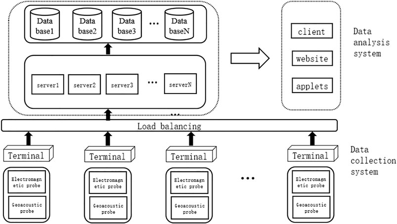
The AETA (Acoustic & Electromagnetics AI) system makes use of electromagnetic disturbance and geo-acoustic signals as observation inputs. It aims to commence imminent earthquake prediction by using large-scale and high-density seismic data as well as well-developed methods from data mining, machine learning, neural network, and relevant fields. The AETA system consists of two parts: 1) the data acquisition subsystem and 2) the data analysis and prediction subsystem.
1) The data acquisition subsystem consists of many AETA stations. Each AETA station is equipped with an electromagnetic sensing probe, a geo-acoustic sensing probe, and a data terminal. Data from the sensing probes will be collected, packed, and transferred to a cloud server. 2) The data analysis subsystem includes a cloud server, a database, a client of data display, a website for data display (https://www.aeta.cn), and our software for real-time seismic prediction. The cloud sever and the database are used for feature extraction and data storage. The software is working to check the data updates and display the predicted outcomes in real time (Figure 1).
In this article, only electromagnetic data are being analyzed in the proposed model. The specifications of the electromagnetic probes are described as follows: the frequency band is 0.1 Hz–10 kHz, the spatio-temporal model of dynamic range is 0.1–1,000 nT, the sensitivity is >20 mV/nT@0.1 Hz–10 kHz, and the sampling rate for the low-frequency band (≤200 Hz) is 500 Hz, which is 30 kHz for the full frequency band (≤10 kHz). Its noises are within 0.1–0.2 pT/Hz@(10 Hz–1 kHz) (Guo et al., 2021).
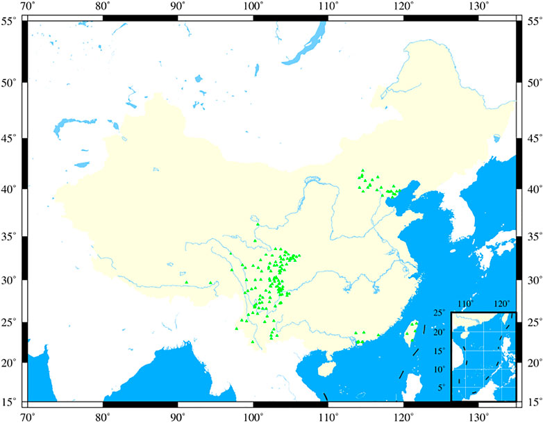
Since January 2017, the AETA team has started constructing the observation network in China (Figure 2). Up to now, more than 300+ stations have been deployed. Most of them are located in the Sichuan-Yunnan region (more than 200 stations, namely, 22°N-34°N and 98°E-107°E) because the region has high seismicity than other places in China (Guo et al., 2021). After 4 years of observations, more than 45 TB of data has been collected, and 20 GB of new data is collected every day. In order to analyze multiple dimensional features, 95 classes of electromagnetic and geo-acoustic signals have been taken into account (Guo et al., 2021). In this article, an average of the electromagnetic data is imported into the proposed model to represent the data in the temporal domain.
Our spatio-temporal model for earthquake prediction
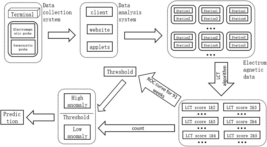
Based on two classes of precursor signals observed by using the AETA system, a new model to predict whether an earthquake will occur in the Sichuan-Yunnan region is proposed. The prediction will be made every Sunday, and the time frame for this prediction is the next 7 days (Figure 3). An LCT algorithm (i.e., local correlation tracking) is being applied to cope with the electromagnetic signals of the AETA system.
LCT algorithm
The proposed LCT method is an improvement of the conventional linear correlation method (Verma et al., 2013). The novelty of this method is that a sliding window in the temporal domain is added, and the correlation between local covariance matrices is calculated in each time window (Schuck, 2005). The correlation calculated by this method in this study is called the LCT correlation.
Regarding time series analysis of electromagnetic signals, at first, a sliding window in the temporal domain xt,ω is applied to segment the data at time t. The window in this article is an exponential decay window, namely, at time t, all windows xt,ω are multiplied by an exponential weight βt−τ. Among them, the window xt,ω closer to the time t will be given a larger exponential weight, while the window far away from the time t will be assigned a smaller weight (Figure 4). Hence, the darker the color, the greater the weight, and vice versa.
Regarding any streaming data X, its local covariance matrix at time t is expressed by Eq. 1.
After calculating the covariance of the two streaming data by using Eq. 1, the local covariance matrix at time t is obtained. After a singular value decomposition (SVD) operation, local covariance matrices
Among them, feature vectors corresponding to the largest eigenvalues are ux and uy. In Eq. 2, U(X) is the left singular vector (LSV) of
Similar to the principal component analysis (PCA) method (Wold et al., 1987), the first few principal components will retain most of the information. Depending on the data distribution, the first k principal components keep the principal feature vector (PFV) matrix. Therefore, the two PFV matrices YX and UY are shown in Eq. 4 and 5, respectively.
Now, there are two spaces span(UY) spanned by UY and span(UX) spanned by UX. Then, multiply ux by using UY at the left side and get
Thus, if two spaces have LCT correlation, θ1 and θ2 approach 0.00, and cos θ1 and cos θ2 will tend to 1.00 as shown in Eq. 8 and 9.
Finally, define the local correlation LocoScoret at time t as shown in Eq. 10.
In summary, the LCT method is applied to calculate the correlation between two streaming data. If there is a large LCT correlation between them, LocoScore should tend to 1.00. On the contrary, if the LCT correlation is small, LocoScore should be close to 0.00.
The analysis of earthquake data by using the LCT method
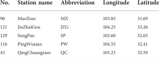
An earthquake (103.82°E, 33.2°N, M7.0) occurred in Jiuzhaigou County, Sichuan Province on 8 August 2017. There are five AETA stations whose geographic locations are near the epicenter (Figure 6 and Table 1), and the low-frequency electromagnetic data collected from these stations 1 month before the earthquake was selected for the analysis.
In order to calculate the correlation coefficient between the data from our stations, it makes use of the classical correlation method and local cross-correlation tracking method to calculate the Pearson correlation coefficient (Jacob et al., 2009).
First, select the electromagnetic disturbance data of No.90 MX station (Figure 7A) and No.75 QW station (Figure 7B) to calculate the Pearson correlation coefficient and LCT correlation coefficient. The data window is from 14 July 2017 to 13 August 2017. From the results (Figure 7), the LCT method has a better output based on non-stationary signals. The classical correlation method cannot reasonably reflect the correlation between the electromagnetic signals from two stations (Figure 7C). If the signals from a station are obviously abnormal, this method cannot be applied to effectively find anomalies.
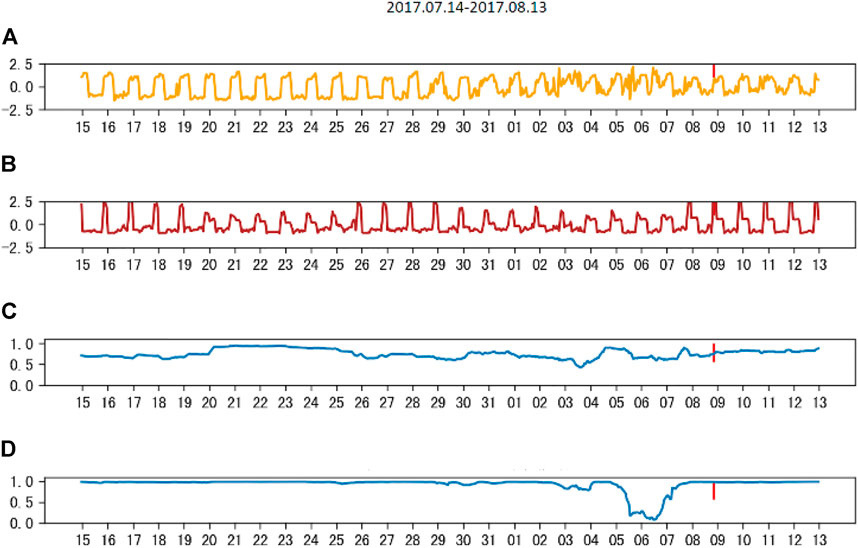
FIGURE 7. (A) Normalized electromagnetic disturbance data of MX station, (B) normalized electromagnetic disturbance data of QW station, (C) the Pearson correlation coefficient between (A) and (B), and (D) LCT correlation coefficient between (A) and (B).
In contrast, the use of the local cross-correlation tracking method can well reflect the correlation between the electromagnetic data of any two stations. Even if very weak signals show anomalies, this method is able to sensitively pick up the anomalies (Figure 7D). In the analysis, the LCT method was employed to calculate the correlation between AETA stations, and the anomaly detected by using this method is called the LCT anomaly, correspondingly.
In order to show that the LCT method is able to find the correlation between AETA electromagnetic data and detect earthquake anomalies, the electromagnetic disturbance data of five AETA stations within 200 km from the epicenter are collected (Figure 8). Although the electromagnetic disturbance data from the No. 43 QC station fluctuate obviously from July 15 to July 25, the signals from these five stations have all been collected in waveform (Figure 8). The electromagnetic disturbance data from each AETA station have anomalies in the week before the earthquake.
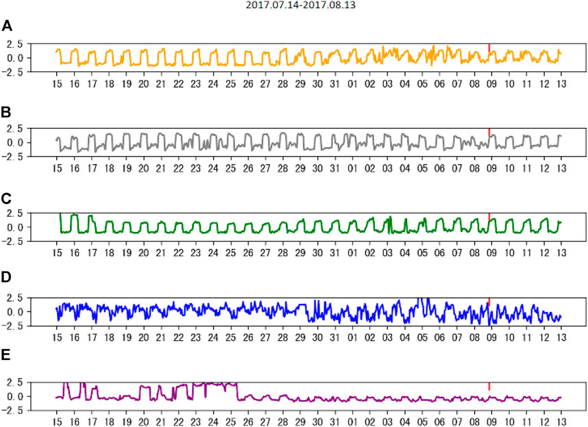
FIGURE 8. Normalized electromagnetic disturbance data from (A) MX, (B) JZG, (C) SP, (D) PW, and (E) QC.
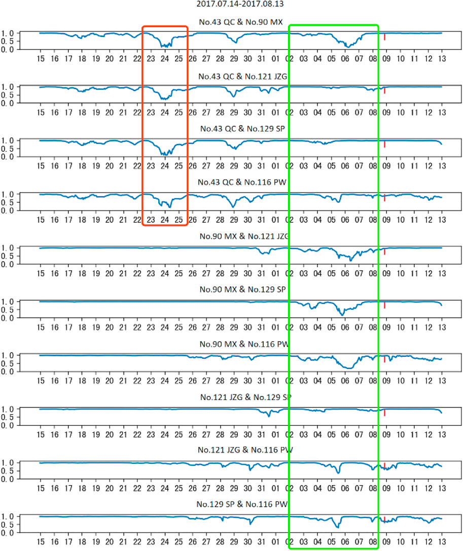
Subsequently, the electromagnetic disturbance data from these five AETA stations were analyzed by using the LCT method, a set of LocoScore scores were calculated between every pair of two stations, and there were a total of
From previous analysis and experimental results (Figure 9), it is found that in the long period of observations before the earthquake, LocoScore between the signals from every two stations is basically close to 1.00, that is, the electromagnetic signals from the stations are the same. The data have good spatial consistency. However, a week before the earthquake, LocoScore between every two stations showed an anomaly of less than 1.00, that is, the original spatial correlation of the electromagnetic data between the two stations was broken by the earthquake. These LCT anomalies reflect precursors related to earthquakes. Based on the analysis, applying the LCT method to AETA electromagnetic disturbance data is able to predict an earthquake.
LCT abnormal calculation
Based on the LCT algorithm, the electromagnetic data from every pair of AETA stations will be applied to an abnormal evaluation, which will be output every day.
First, define the LCT anomaly: the electromagnetic data from multiple AETA stations will be analyzed by using the LCT method to calculate the LocoScore of each pair of stations before the earthquake and a total of 10 days after the earthquake. According to the choice of the time window, there will be different LocoScore values.
There are 24 values in the LocoScore per hour per day for a total of 24 × 10 = 240 values in 10 days. Thus, define the anomaly of each day as LocoScoreDay (Figure 10) or day-based.
Therefore, the abnormal results of LCT will be output every day. The median of the daily LocoScore is selected as the outlier of the two stations per day.
Large-scale application of the LCT method
By using the LCT method of AETA, an outlier is able to be obtained from the data of the two stations every day. The outlier is between [0,1.00]. The smaller the value, the more serious the abnormal situation between the data of these two stations. There are 80 stations that were selected after removing those stations with frequent failures or with unchanged signals, and get
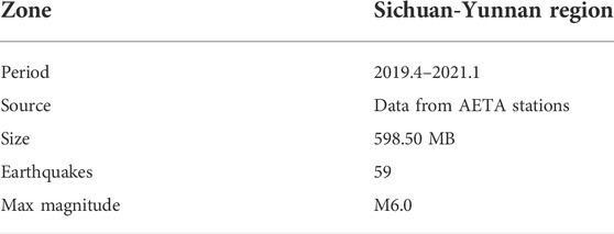
The specifications in this work from the different datasets for the model were extracted.
Weekly earthquake prediction in the Sichuan-Yunnan region
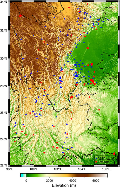
The LCT anomalies were calculated based on AETA electromagnetic disturbance data for 21 months (91 weeks) in the Sichuan-Yunnan region from 22 April 2019 to 24 January 2021. During this period of time, the distribution of earthquakes and AETA stations (Figure 11). The red dots indicate the epicenter, and the blue dots show the AETA station.
The daily LCT abnormal times in the Sichuan-Yunnan area for 1 week are counted, then look for the value threshold Val ∈ R and the number threshold Num ∈ Z+ of daily anomalies, and review all of them every Sunday. If the times of LCT abnormalities whose values are lower than Val on a day of this week exceed Num, it is considered that there will be an earthquake of M3.5 or higher in the next week. Otherwise, it is predicted that there will be no earthquakes next week. For example, let’s assume Num=20. A one-week review was conducted on Sunday (3 January 2021), and the LCT anomalies from 28 December 2020 to 3 January 2021 were counted. It is found that on 30 December 2020, the number of anomalies below 0.08 was 48. More than 20, we predict that the next week from 4 January 2021 to 10 January 2021, there will be an earthquake in the region (Table 2). A suitable Num will be found so that the outcome of using LCT anomalies to predict weekly earthquakes is the best. By using the ROC curve to analyze and calculate, the Num result is 30.
ROC curve
ROC curve refers to the receiver operating characteristic (ROC) curve. The ROC curve is a diagram composed of the false alarm probability as the horizontal axis and the hit probability as the vertical axis; the curve is drawn by different results obtained by the subjects under specific stimulus conditions due to different judgment standards (Molchan, 2010; Mirmiran et al., 2004).
The hit rate in the ROC curve is the proportion of positive samples in the test set that are correctly classified. The false-positive rate in the ROC curve is the proportion of negative samples in the test sample set that are incorrectly identified (Kamarudin et al., 2017).
For a dataset, each classification model has a ROC curve (Calì and Longobardi, 2015). The classification model follows a rule, usually, a threshold. The hit rate and false alarm rate of this threshold based on the sample set are obtained, so as to mark a point on the ROC curve, it could continuously adjust the threshold of the classification model and mark the points on the ROC map, and these points are connected to the ROC curve of this classification model based on this sample set.
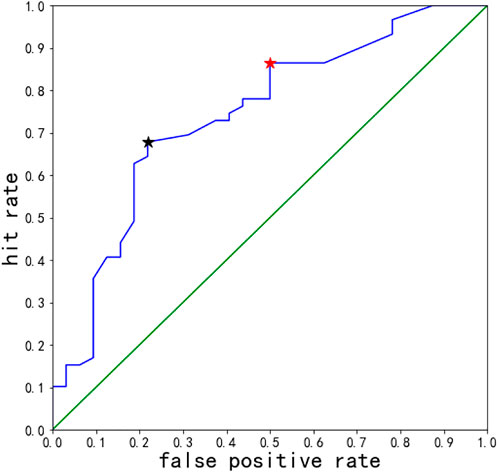
For the classification results by using the LCT method, a threshold is needed to be fixed. If the threshold is exceeded, the sample is judged as an earthquake sample; otherwise, it is judged as a no-earthquake sample. We make use of the number of anomalies to make judgments. For our dataset, if the earthquake magnitude is higher than M3.5, the week is defined as a positive week, while the weeks without earthquakes are treated as negative weeks (Figure 12).
Obviously, if the threshold is 0.00, all samples are judged as positive samples. At this time, the hit rate is 1.00, and the false alarm rate is 1.00, corresponding to the points at (1.00, 1.00) in the top-right corner. If the threshold is set at infinity, all samples are judged as negative samples. At this time, the hit rate is 0.00, and the false alarm rate is 0.00, corresponding to the points at (0.00, 0.00) in the bottom-left corner. The remaining points on the blue line correspond to other thresholds. As the threshold continues to increase, the corresponding points move along the blue line from the top-right to the bottom-left corner. A small drop in false alarm rates is a tradeoff with a drop in hit rates. The most ideal point is the point at the top-left corner. The hit rate is 1.00, and the false alarm rate is 0.00, which means this classification model completely distinguishes between positive and negative samples. The closer to the upper left corner, the better the threshold.
The red star and the black star (Figure 12) are the closest ones to the top-left corner. The threshold related to the red star is 8, and the threshold corresponding to the black star is 30. The coordinates of the red star are (0.50, 0.86), while those of the black star are (0.22, 0.69). The distance from (0, 1.00) is 0.52 for the red star and 0.37 for the black star. The classification result with the threshold of 30 corresponding to the black star is better.
The AUC value of the classifier for the number of abnormal points in the LCT model, which is the area under the diagonal line, is calculated easily (Kamitsuji and Kamatani, 2006; Lever et al., 2016) (Figure 12) as 0.74, far exceeding 0.50. This is a good result in earthquake prediction. With the AUC value, it can be concluded that LCT anomalies have a considerable correlation, which proves that LCT anomalies are effective in predicting earthquakes that will occur in a few days.
To sum up, first, use the LCT method to analyze the electromagnetic signals from the AETA station, get the signal anomalies between two stations every day, and count the number of abnormal values below 0.08. A weekly review is carried out every Sunday. If this week has anomalies and the number of anomalies for this week is greater than or equal to 30, it is predicted that an earthquake will occur in this region next week; otherwise, it is predicted that no earthquake will occur.
Prediction result analysis
The ROC curve can be used to find the optimal and sub-optimal amounts of data and draw a prediction chart based on this. Therefore, earthquakes can be predicted more intuitively (Figure 13). The abscissa is the number of weeks in chronological order, and the ordinate is the number of LCT outliers less than 0.08. The blue discount indicates the actual occurrence of earthquakes in the 91 weeks, 0 means no earthquake occurred this week, and non-zero means an earthquake occurred this week. The black horizontal line represents the threshold represented by the black star (Figure 13), which is 30. The red broken line represents the number of days with the largest number of LCT outliers of less than 0.08 this week. If the red broken line is lower than the black horizontal line, it will be predicted that there will be no earthquakes; otherwise, the occurrence of earthquakes will be predicted. Compared with the blue broken line, which indicates the actual occurrence of the earthquake, the yellow area is to indicate whether the earthquake is correctly predicted (Figure 14, Figure 13). The threshold presented by using a black horizontal line has been changed to 9, which corresponds to the threshold represented by the red star (Figure 12), the correct prediction time has also been replaced by a light green block, and the orange color block indicates the time if both thresholds are correctly predicted (Figure 15).
It is clear that no matter whether the threshold is 8 or 30, the number of correct predictions of earthquake occurrence far exceeds the number of incorrect predictions (Figures 13–15). This also reflects that LCT anomalies indeed predict earthquakes much more accurately, and there is definitely a greater correlation between them and earthquakes.
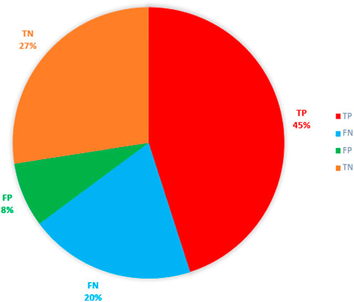
To verify whether there will be an earthquake prediction next week, we may get four results (Asencio-Cortés et al., 2015). In this article, we treat earthquakes as positive samples and no earthquakes as negative samples. TP and TN mean the prediction is correct. The results are shown (Table 3, Table 4 and Figure 16).
In this article, we propose the metrics to measure the quality of the forecast results.
By calculating P=0.85, A=0.73, R=0.69, and F=0.23, where TP is a true positive or hit, FN is a false negative or the miss, FP is a false positive or false alarm, and TN is a true negative or correct rejection. Meanwhile, Pre is the precision, Rec is the recall, Acc is the accuracy, and Fpr is the false positive rate.
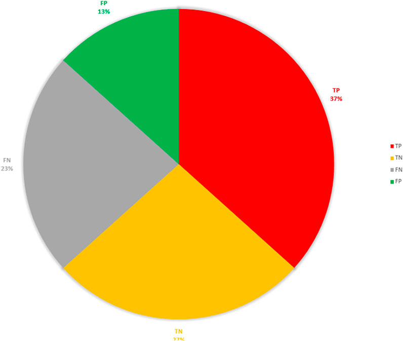
The earthquake prediction results in real time for a total of 30 weeks from 1 April 2021 to 31 October 2021 can also be calculated and published on the AETA prediction platform website, open to visitors from all over the world. During the 30 weeks, there were 15 weeks of actual earthquakes in the Sichuan-Yunnan area and 15 weeks without earthquakes. The system gives 18 earthquake predictions and 12 earthquake-free predictions. The prediction results are shown in Table 5 and Figure 17.
Conclusion
Our work is designing and developing AETA systems based on the deployed stations first. Since January 2017, we have started creating an observation network in China. Up to now, more than 300 stations have been deployed. Most of them are located in the Sichuan-Yunnan region in China, with more than 200 stations, which collect a huge amount of low-frequency electromagnetic data.
Second, based on the low-frequency electromagnetic signals observed by using the AETA system, the LCT method is applied to analyze, calculate, and process the correlation between the local covariance matrices corresponding to each time window of the two streaming data. The daily anomalies by using the LCT method can be calculated. By counting the number of abnormal values below the threshold of 0.08 and conducting a weekly review every Sunday, an earthquake can be predicted to occur in the region next week.
Finally, based on the LCT abnormal analysis from the electromagnetic disturbance data of AETA, the ROC curve is employed to analyze the prediction outcomes of the LCT model in 91 weeks. Key metrics such as hit rate, false alarm rate, and AUC value are proposed. The ROC curve for earthquake prediction of each classifier was drawn, and the data of earthquakes were analyzed. It proves that the LCT anomaly and the earthquake have a considerable correlation, the optimal threshold was found, and the classification results were evaluated, respectively. Finally, four metrics are introduced to measure the LCT method based on earthquake prediction classification, which proves its excellent performance for classification.
Data availability statement
The original contributions presented in the study are included in the article/Supplementary Material; further inquiries can be directed to the corresponding author.
Author contributions
JX: data curation, formal analysis, writing—draft, software, and methodology. SY: project administration and writing—review. XW: funding acquisition, investigation, and project administration. Others: support.
Conflict of interest
The authors declare that the research was conducted in the absence of any commercial or financial relationships that could be construed as a potential conflict of interest.
Publisher’s note
All claims expressed in this article are solely those of the authors and do not necessarily represent those of their affiliated organizations, or those of the publisher, the editors, and the reviewers. Any product that may be evaluated in this article, or claim that may be made by its manufacturer, is not guaranteed or endorsed by the publisher.
Supplementary material
The Supplementary Material for this article can be found online at: https://www.frontiersin.org/articles/10.3389/feart.2022.902745/full#supplementary-material
References
Asencio-Cortés, G., Martínez-Álvarez, F., Morales-Esteban, A., Reyes, J., and Troncoso, A. (2015). “Improving earthquake prediction with principal component analysis: Application to Chile,” in Hybrid artificial intelligent systems. Editors E. Onieva, I. Santos, E. Osaba, H. Quintián, and E. Corchado (Cham: Springer International Publishing), 393–404.
Calì, C., and Longobardi, M. (2015). Some mathematical properties of the roc curve and their applications. Ric. Mat. 64 (2), 391–402. doi:10.1007/s11587-015-0246-8
Chadha, R. K., Pandey, A. P., and Kuempel, H. J. (2003). Search for earthquake precursors in well water levels in a localized seismically active area of reservoir triggered earthquakes in India. Geophys. Res. Lett. 30 (7). doi:10.1029/2002gl016694
Freund., F. (2010). Toward a unified solid state theory for pre-earthquake signals. Acta Geophys. 58 (5), 719–766. doi:10.2478/s11600-009-0066-x
Guo, Q., Yong, S., and Wang, X. (2021). Statistical analysis of the relationship between aeta electromagnetic anomalies and local earthquakes. Entropy 23 (4), 411. doi:10.3390/e23040411
Jacob, B., Chen, J., Huang, Y., and Cohen, I. (2009). Pearson correlation coefficient. Berlin, Heidelberg: Springer Berlin Heidelberg, 1–4.
Jónsson, S., Paul, S., Pedersen, R., and Björnsson, G. (2003). Post-earthquake ground movements correlated to pore-pressure transients. Nature 424 (6945), 179–183. doi:10.1038/nature01776
Kamarudin, A. N., Cox, T., and Kolamunnage-Dona, R. (2017). Time-dependent roc curve analysis in medical research: Current methods and applications. BMC Med. Res. Methodol. 17 (1), 53. doi:10.1186/s12874-017-0332-6
Kamitsuji, S., and Kamatani, N. (2006). Estimation of haplotype associated with several quantitative phenotypes based on maximization of area under a receiver operating characteristic (roc) curve. J. Hum. Genet. 51 (4), 314–325. doi:10.1007/s10038-006-0363-z
Keilis-Borok, V., Shebalin, P., Gabrielov, A., and Turcotte, D. (2004). Reverse tracing of short-term earthquake precursors. Phys. earth Planet. interiors 145 (1-4), 75–85. doi:10.1016/j.pepi.2004.02.010
Lever, J., Martin, K., and Altman, N. (2016). Classification evaluation. Nat. Methods 13 (8), 603–604. doi:10.1038/nmeth.3945
Martinelli, G., Plescia, P., and Tempesta, E. (2020). Electromagnetic emissions from quartz subjected to shear stress: Spectral signatures and geophysical implications. Geosci. Switz. 10, 140. doi:10.3390/geosciences10040140
Martinelli, G., Plescia, P., and Tempesta, E. (2020). pre-earthquake” micro-structural effects induced by shear stress on α-quartz in laboratory experiments. Geosciences 10, 155. doi:10.3390/geosciences10050155
McGuire, J. J., Boettcher, M. S., and Jordan, T. H. (2005). Foreshock sequences and short-term earthquake predictability on east Pacific rise transform faults. Nature 434 (7032), 457–461. doi:10.1038/nature03377
Mirmiran, P., Esmaillzadeh, A., and Azizi, F. (2004). Detection of cardiovascular risk factors by anthropometric measures in tehranian adults: Receiver operating characteristic (roc) curve analysis. Eur. J. Clin. Nutr. 58 (8), 1110–1118. doi:10.1038/sj.ejcn.1601936
Molchan, G. (2010). Space—time earthquake prediction: The error diagrams. Basel: Springer Basel, 53–63.
Moreno, M., Rosenau, M., and Oncken, O. (2010). 2010 Maule earthquake slip correlates with pre-seismic locking of Andean subduction zone. Nature 467 (7312), 198–202. doi:10.1038/nature09349
Olson, E. L., and Allen, R. M. (2005). The deterministic nature of earthquake rupture. Nature 438 (7065), 212–215. doi:10.1038/nature04214
Pulinets, S., and Ouzounov, D. (2011). Lithosphere–atmosphere–ionosphere coupling (laic) model–an unified concept for earthquake precursors validation. J. Asian Earth Sci. 41 (4-5), 371–382. doi:10.1016/j.jseaes.2010.03.005
Roger, B. (2010). Lessons from the Haiti earthquake. Nature 463 (7283), 878–879. doi:10.1038/463878a
Schorlemmer, D., and Wiemer, S. (2005). Microseismicity data forecast rupture area. Nature 434 (7037), 1086. doi:10.1038/4341086a
Schuck, P. W. (2005). Local correlation tracking and the magnetic induction equation. Astrophys. J. 632 (1), L53–L56. doi:10.1086/497633
Uyeda, S., Nagao, T., and Kamogawa, M. (2011). Earthquake precursors and prediction. Encycl. Solid Earth Geophys. 1, 168–178. doi:10.1007/978-90-481-8702-7_4
Verma, M., Steffen, M., and Denker, C. (2013). Evaluating local correlation tracking using co5bold simulations of solar granulation. Astron. Astrophys. 555, A136. doi:10.1051/0004-6361/201321628
Wold, S., Kim, E., and Paul, G. (1987). Principal component analysis. Chemom. Intell. Lab. Syst. 2 (1), 37–52. doi:10.1016/0169-7439(87)80084-9
Keywords: earthquake prediction model, ROC curve, AETA system, singular value decomposition, local correlation tracking
Citation: Xie J, Yong S, Wang X, Bao Z, Liu Y, Zhang X and He C (2022) Weekly earthquake prediction in a region of China based on an intensive precursor network AETA. Front. Earth Sci. 10:902745. doi: 10.3389/feart.2022.902745
Received: 23 March 2022; Accepted: 26 August 2022;
Published: 28 September 2022.
Edited by:
Giovanni Martinelli, National Institute of Geophysics and Volcanology, ItalyReviewed by:
Alexey Lyubushin, Institute of Physics of the Earth (RAS), RussiaPaolo Plescia, National Research Council (CNR), Italy
Copyright © 2022 Xie, Yong, Wang, Bao, Liu, Zhang and He. This is an open-access article distributed under the terms of the Creative Commons Attribution License (CC BY). The use, distribution or reproduction in other forums is permitted, provided the original author(s) and the copyright owner(s) are credited and that the original publication in this journal is cited, in accordance with accepted academic practice. No use, distribution or reproduction is permitted which does not comply with these terms.
*Correspondence: Shanshan Yong, eW9uZ3NoYW5zaGFuQHBrdS5lZHUuY24=
 Jinhan Xie
 Shanshan Yong2*
 Zhenyu Bao