The Virtual Element Method for the Dam Foundation With Joint

The contact is a typical non-linear problem that exists in various projects. For traditional three-node triangular mesh and four-node quadrilateral mesh, the accuracy and convergence of the calculation results are affected by the quality of the mesh. The test space and trial space in the virtual element method (VEM) do not need to be accurately calculated, avoiding mesh dependence. In this paper, the formulation of linear elasticity and the formulation of the frictionless node-to-segment (NTS) contact model via VEM are shown. There are four numerical simulations. The sensitivity of the virtual element method to mesh distortion is studied in the first numerical simulation. The exactness and convergence of the algorithm are investigated by the second numerical example. The second numerical example simultaneously explores the penalty factor’s effect on the results. The third example investigated the impact of mesh shape and number of Voronoi mesh elements on the results by comparing normal contact stresses. The fourth numerical example studies the application of the method to engineering. Those numerical examples show that the virtual element method is insensitive to mesh distortion and could solve the joint contact in engineering.

1 Introduction

The contact problem is a typical nonlinear problem, widespread in actual engineering such as geotechnical engineering, building structure, water project, and machinery engineering. In the past 2 decades, with the development of electronic computers and the rise and development of various numerical methods, there are powerful means to handle the contact problems such as finite element method (FEM), numerical manifold method (NMM) (Yang et al., 2019; Zheng et al., 2019; Yang et al., 2020a; Yang et al., 2020b; Yang et al., 2021a; Yang et al., 2021b), boundary element method (BEM).

For those numerical methods, FEM has been the greatest broadly utilized. Hughes (Hughes et al., 1976) and Francavilla (Padmanabhan and Laursen, 2001) are considered pioneers who solve the contact problem by using FEM. In order to improve the classical contact discretization, there are some methods that have been studied, which are based on constraint element node enforcement. (Hautefeuille et al., 2012; Khoei et al., 2006; Wriggers et al., 2001). More recently, some researchers (Wriggers et al., 2001; da Veiga et al., 2014; Sheng and Yuan, 2012; Krstulovic-Opara et al., 2002; Liu et al., 2007; Flemisch et al., 2005) prefer the mortar method for the discretization of contact constraints. The stable interpolation condition for contact constraints is provided by those methods because of the weak form based on the mortar method. What is known to us is that the gradient of the FEM with a standard degree of freedom is not continuous on internal element edges. When FEM is employed, it has been proved that results are highly sensitive to mesh quality (Lee and Bathe, 1993; Liu et al., 2007; Yang et al., 2014). For contact problems, the results are influenced by the quality of the meshes where they are in the possible contact area. When the contact boundary between two contact bodies is irregular, the calculation results using FEM are greatly affected.

Because of the insufficient FEM, the VEM is proposed by Brezzi (Beirão Da Veiga et al., 2013). Since the birth of the VEM, it has been applied in many aspects by many scholars. The two-dimensional Poisson problem that is discretized by polygonal discretization is solved by VEM (Sutton, 2017). In the VEM framework, the maximum entropy basis function is employed to settle the Poisson problem and linear elastic problem by Ortiz-Bernardin (Ortiz-Bernardin et al., 2017). Sun and Lin (Sun et al., 2020) studied the stability of stony soil slope under excavation using VEM. However, there are few papers that solve the contact problem by VEM.

The contact constraint is commonly handled by the Lagrange multiplier method (LMM) (Béchet et al., 2010; Hautefeuille et al., 2012), the penalty method (PM) (Liu and Borja, 2008; Liu and Borja, 2010a; Liu and Borja, 2010b), and the augmented Lagrange method (ALM). The PM can convert the non-linear contact problem into material nonlinearity. The advantage of the PM is that the global system is not extended when the contact conditions are introduced. The disadvantage of PM is that the contact constraints can be satisfied approximately. The contact constraint can be satisfied accurately. However, the global system needs to be extended by an additional variable for the Lagrange multiplier. To evade the disadvantages of PM and LMM, the ALM was proposed. However, there are sub-iterations in each calculation step in the ALM, which is its primary deficiency. This paper aims to find the solution to the contact problem in engineering, and the result of PM can fully meet the needs of engineering. In summary, the contact constraint is handled by PM in this paper.

The rest of this article is composed of the following parts. The application of the lowest order VEM for the linear elasticity problem is presented in Section 2 and Section 3 shows the NTS contact model. In Section 4, the numerical examples are given for performances of the VEM in different situations, including the response to mesh quality, the performance of normal contact pressure in Hertzian contact, the influence of varying mesh shapes for the normal contact pressure in the horizontal contact interface and the application of algorithms in engineering. The discussion and concluding remarks are presented in Section 5 and Section 6, respectively.

2 Linear Elasticity

2.1 The Model

The elastic body is composed of an open domain $\text{Ω}\subseteq R^2$. The Dirichlet boundary and Neumann boundary are represented by ${\text{Γ}}_g$, ${\text{Γ}}_t$. The displacement field of the elastic body can be represented by $u\left(x\right)$. The Dirichlet boundary conditions are $g\left(x\right)$. The linear elastic boundary-value problem can be expressed that discovering $u\left(x\right)$ satisfies the following conditions (Ortiz-Bernardin et al., 2017):

$\{\begin{array}{c}\nabla \mathit{\sigma }+\mathit{b}=0\\ \begin{array}{cc}\mathit{u}=g& g\in {\text{Γ}}_g\end{array}\\ \begin{array}{cc}\mathit{\sigma }\cdot \mathit{n}=\mathit{t}& b\in {\text{Γ}}_t\end{array}\end{array}$(2.1)

Where $\mathit{\sigma }$ represents the stress tensor, $\mathit{b}$ is the body force, $\mathit{n}$ is the unit normal of boundary, the $\mathit{t}$ is the external traction. The equivalent Calerkin variational formulation can be expressed that finding $\mathit{u}\mathit{\subset }\mathit{U}$ satisfies the equation

$\begin{array}{c}a\left(\mathit{u},\mathit{v}\right)=l\left(\mathit{u},\mathit{v}\right)u\subset U,v\subset V\\ a\left(\mathit{u},\mathit{v}\right)={\displaystyle \underset{\text{Ω}}{\int }\sigma \left(\mathit{u}\right)}:\epsilon \left(v\right)d\text{Ω}\\ l\left(\mathit{v}\right)={\displaystyle \underset{\text{Ω}}{\int }b\cdot \mathit{v}d\text{Ω}}+{\displaystyle \underset{{\text{Γ}}_t}{\int }t\cdot \mathit{v}d\text{Γ}}\end{array}$(2.2)

Where $\mathit{V}$ and $\mathit{U}$ represent the displacement test and trial space.

2.2 Discrete Bilinear Form

The domain $\text{Ω}$ is divided into non-overlapping polygonal elements that make up the area ${\text{Γ}}_h$.

The virtual function space is defined to be

$V_h:=\left\{v\in {\mathit{H}}^1\left(E\right):{v|}_E\in V_h^{E}forallE\in {\text{Γ}}_h\right\}$(2.3)

Where $V_h^E$ is the local space on the element $E.$ $V_h^E$ sustains some properties (Sutton, 2017).

The basis function of space $V_h^E={\left({\mathit{V}}_{\mathit{h}}^{\mathit{E}}\right)}^2$ can be expressed as $\overline{{\varphi }_1},\cdots ,\overline{{\varphi }_N},\cdots ,\underset{¯}{{\varphi }_1}\cdots \underset{¯}{{\varphi }_N}$.

$\overline{{\varphi }_i}=\left[\begin{array}{c}{\varphi }_i\\ 0\end{array}\right],\underset{¯}{{\varphi }_i}=\left[\begin{array}{c}0\\ {\varphi }_i\end{array}\right],i=1,\cdots N$

For any $\mathit{u}=\left(u_1,u_2\right)=:\left(\overline{u},\underset{¯}{u}\right)\in {\mathit{V}}_{\mathit{h}}^{\mathit{E}}$.

$\mathit{u}={\displaystyle \sum _{i=1}^N\overline{u_i}\overline{{\varphi }_i}}+{\displaystyle \sum _{i=1}^N\underset{¯}{u_i}\underset{¯}{{\varphi }_i},\overline{u_i}}={\chi }_i\left(\overline{u}\right),\underset{¯}{u_i}={\chi }_i\left(\underset{¯}{u}\right)$

Therefore

$do{f}_i\left(\mathit{u}\right)={\chi }_i\left(u_1\right),do{f}_{i+N}\left(\mathit{u}\right)={\chi }_i\left(u_2\right)$

The basis function of polynomial space ${\mathit{P}}_{\mathit{E}}={\left(P_E\right)}^2$ can be expressed as (Nguyen-Thanh et al., 2018). ${\mathit{P}}_{\mathit{E}}$ is a subspace of ${\mathit{V}}_{\mathit{h}}^{\mathit{E}}$.

$\left[\overline{m_1},\overline{m_2},\overline{m_3},\underset{¯}{m_1},\underset{¯}{m_2},\underset{¯}{m_3}\right]$(2.4)

$\overline{m_{\alpha }}=\left[\begin{array}{c}{m}_{\alpha }\\ 0\end{array}\right],\underset{¯}{m_{\alpha }}=\left[\begin{array}{c}0\\ m_{\alpha }\end{array}\right],\alpha =\mathrm{1,2,3}$

We can define a projection from the virtual function space to the polynomial space ${\text{Π}}^E:{\mathit{V}}_{\mathit{h}}^{\mathit{E}}\to {\mathit{P}}_{\mathit{E}}$. The defined projection needs to satisfy the following equation:

$a_h^E\left({\text{Π}}^E\mathit{v},\mathit{p}\right)=a_h^E\left(\mathit{v},\mathit{p}\right),\mathit{p}\in {\left({\mathit{P}}_{\mathit{E}}\right)}^2$(2.5)

${\displaystyle \underset{\partial E}{\int }{\text{Π}}^E\mathit{v}dS}={\displaystyle \underset{\partial E}{\int }\mathit{v}dS}$(2.6)

The defined vectors form is

${\displaystyle \underset{\mathit{E}}{\int }\nabla {\mathit{m}}^T\cdot \nabla {\text{Π}}^E\mathit{\varphi }dx}={\displaystyle \underset{E}{\int }\nabla {\mathit{m}}^T\cdot \nabla \mathit{\varphi }dx}$(2.7)

$P_0\left(\nabla {\text{Π}}^E\mathit{\varphi }\right)=P_0\left(\mathit{\varphi }\right)$(2.8)

Where $P_0$ is the constant term projection operator (Sutton, 2017).

2.2 Element Stiffness Matrix

Due to $P_E\subset V_h^E$, The equation can be obtained

$\mathit{m}=\mathit{D}\mathit{\varphi }$(2.9)

Where $\mathit{D}$ represents the expression of the matrix under the basis function $\mathit{\varphi }$.

Additionally, on account of ${\text{Π}}^E\mathit{\varphi }\mathit{\in }{\mathit{P}}_{\mathit{E}}\subset V_h^E$, The equation can be obtained

${\text{Π}}^E{\varphi }_i{\displaystyle \sum _{\alpha =1}^{N_E^k}{a}_{i,\alpha }{\varphi }_{\alpha }}={\displaystyle \sum _{j=1}^{N_E^k}{s}_{i,j}{m}_j}$(2.10)

From the Eq. 2.9, the equation is obtained

${\displaystyle \sum _{\alpha =1}^{N_E^k}{\mathit{s}}_{\alpha }}={\displaystyle \sum _{j=1}^{N_E^k}{D}_{\alpha ,j}{a}_j}$(2.11)

The equations of Eq. 2.11 and Eq. 2.10 are brought into Eq. 2.2, and the following equation is obtained

$\overline{\mathit{G}}\mathit{S}=\overline{\mathit{B}}$(2.12)

The matrixes of $\overline{\mathit{G}}$ and $\overline{\mathit{B}}$ are computed as follows

$\overline{G_{\alpha ,\beta }}=\{\begin{array}{c}{P}_0\left(m\right)if\beta =1\\ {\displaystyle \underset{E}{\int }\nabla m_{\alpha }\cdot \nabla m_{\beta }dx}\end{array}$

$\overline{B_{\beta ,j}}=\{\begin{array}{c}{P}_0\left(\varphi \right)if\beta =1\\ {\displaystyle \underset{E}{\int }\nabla {\varphi }_{\alpha }\cdot \nabla m_{j}dx}\end{array}$

Eq. 2.10 can be written as a matrix expression as

$\overline{\mathit{G}}=\overline{\mathit{B}}\mathit{D}$(2.13)

Bring Eq. 2.13 into Eq. 2.12

$\mathit{S}={\left(\overline{\mathit{B}}\mathit{D}\right)}^{-1}\overline{\mathit{B}}$(2.14)

The element stiffness matrix is (Beirão da Veiga et al., 2014)

${\left(K_E\right)}_{ij}=a\left({\text{Π}}^{E}u,{\text{Π}}^{E}v\right)+a\left(u-{\text{Π}}^{E}u,v-{\text{Π}}^{E}v\right)={\left(\nabla {\text{Π}}^E{\varphi }_{i,}\nabla {\text{Π}}^E{\varphi }_j\right)}_{0,E}+{\left(\nabla \left(1-\nabla {\text{Π}}^E{\varphi }_{i,}\right),\nabla \left(1-\nabla {\text{Π}}^E{\varphi }_j\right)\right)}_{0,E}$(2.15)

The meaning of the Eq. 2.15 can refer to the articles (Chen, 2015; Ortiz-Bernardin et al., 2017).

3 The Contact Problem for VEM

3.1 Description of Different Contact Condition

Figure 1 presents a two-dimensional frictionless contact model. For domain ${\text{Ω}}_1$ and ${\text{Ω}}_2$, the possible contact boundaries are $S_1$ and $S_2$, g represents the contact gap. let $R_1$ and $R_2$ are the contact force vectors in the contact region.

FIGURE 1

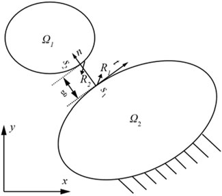
FIGURE 1. Contact problem description.

Consider $d{S}_1$ and $d{S}_2$ are the infinitesimal region where is coming into contact. The virtual work $\delta W$ done by the contact traction is

$\delta W={\displaystyle \underset{S_1}{\int }{\mathit{R}}_1\cdot \delta {\mathit{u}}_{1}d{S}_1}+{\displaystyle \underset{S_2}{\int }{\mathit{R}}_2\cdot \delta {\mathit{u}}_{2}d{S}_2}$(3.1)

In the contact area, every point should satisfy the equilibrium equation

${\mathit{R}}_{1}d{S}_1={\mathit{R}}_{2}d{S}_2$(3.2)

Thus, we could consider the integral in Eq. 3.1 along the contact line $S_1$ or $S_2$.

$\delta W={\displaystyle \underset{S_1}{\int }{\mathit{R}}_1\cdot \left(\delta {\mathit{u}}_1-\delta {\mathit{u}}_2\right)d{S}_1}$(3.3)

3.2 NST Contact Model

In this paper, the NST contact model is employed. A mapping is defined in Figure 2.

FIGURE 2

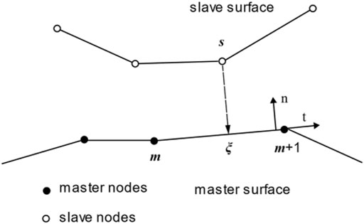
FIGURE 2. NTS contact model.

In the Figure 2, the tangent vector and normal vector of the master element establish a local coordinate system $\left(\mathit{n},\mathit{t}\right)$. The $\mathit{t}$ can be written in matrix form as

$\mathit{t}=\frac{\left|\begin{array}{c}{x}_{m+1}-x_m\\ y_{m+1}-y_m\end{array}\right|}{l}$

The $\mathit{n}$ is

$\mathit{n}=\frac{\left|\begin{array}{c}{y}_m-y_{m+1}\\ x_{m+1}-x_m\end{array}\right|}{l}$

Where $l$ stands for the length of node $m+1$ to $m$ and $\left(x_m, y_m\right)$ is coordinates of node $m$.

The projection node coordinates of node $s$ is on the surface composed of nodes $m$ and $m+1$ is

$\xi =\frac{\left({\mathit{x}}_{\mathit{m}+1}-{\mathit{x}}_{\mathit{m}}\right)\cdot \left[{\mathit{x}}_{\mathit{s}}-{\mathit{x}}_{\mathit{m}}\right]}{l}$(3.4)

The relative displacement from node $s$ to the corresponding segment could be calculated as

${\mathit{u}}_{\mathit{s}}-{\mathit{u}}_{\mathit{\xi }}=\left[\begin{array}{c}10\xi 01-\xi 0\\ 010\xi 01-\xi \end{array}\right]\left[\begin{array}{c}{x}_s\\ y_s\\ x_m\\ y_m\\ x_{m+1}\\ y_{m+1}\end{array}\right]=A\left(\xi \right)\mathit{x}$(3.5)

The $g_s$ indicates the normal gap, and it can be computed by the following equation

$g_s={\mathit{n}}^T\cdot u$(3.6)

Bring the Eq. 3.5 into Eq. 3.3, The contact integral can be calculated

$\delta W={\displaystyle \underset{S_1}{\int }{\mathit{R}}_1\cdot \delta \left({\mathit{u}}_{\mathit{s}}-{\mathit{u}}_{\mathit{\xi }}\right)d{S}_1}$(3.7)

The $\delta u_1$ is replaced by $\delta u_s$ and $\delta u_2$ is replaced by $\delta u_{\xi }$. The contact force $R_1$ can be split into

${\mathit{R}}_1=\mathit{N}+\mathit{T}=N\cdot \mathit{n}+T\cdot \mathit{t}$(3.8)

In the frictionless contact problem, the tangential part disappears $\left(T=0\right)$. Thus, the integral of Eq. 3.7 can be written as

$\delta W={\displaystyle \underset{S_1}{\int }{\mathit{R}}_1\cdot \delta \left({\mathit{u}}_{\mathit{s}}-{\mathit{u}}_{\mathit{\xi }}\right)d{S}_1=}{\displaystyle \underset{S_1}{\int }{\mathit{R}}_1\cdot \mathit{n}\delta g_{s}d{S}_1}={\displaystyle \underset{S_1}{\int }\mathit{N}\delta g_{s}d{S}_1}$(3.9)

3.3 Penalty Method

When the PM is employed for the frictionless contact problem, contact traction $\mathit{N}$ can be written as

$N={\omega }_{N}H\left(-g_s\right)g_{s}withH\left(-g_s\right)=\{\begin{array}{cc}0& if{g}_s>0\\ 1& if{g}_s\le 0\end{array}$(3.10)

Thus, the Eq. 3.9 can be written as

$\delta W={\displaystyle \underset{S_1}{\int }{\omega }_{N}H\left(-g_s\right)g_s\delta g_{s}d{S}_1}$(3.11)

Using numerical methods to catch the ball nonlinear problems, like contact problems, solved by iterative methods. The method requires the derivatives of the weak form $\delta W$. This method is called linearization.

Differentiating Eq. 4–13 with respect to time $t$, we get

$\begin{array}{c}\frac{d\delta W}{dt}=\frac{d\delta W_N}{du}\frac{du}{dt}={\omega }_{N}f\left({\xi }^3\right)\dot{{\xi }^3}\delta {\xi }^3\\ ={\omega }_{N}f\left({\xi }^3\right)\left({\mathit{v}}_{\mathit{s}}-{\mathit{v}}_{\mathit{m}}\right)\cdot \mathit{n}\cdot \delta {\mathit{x}}^{\mathit{T}}\cdot A^T\cdot \mathit{n}\\ ={\omega }_{N}f\left({\xi }^3\right)\delta {\mathit{x}}^{\mathit{T}}{A}^T\mathit{n}\mathit{\otimes }\mathit{n}\cdot A\cdot \mathit{v}\end{array}$(3.12)

Without considering the rotation of the contact body, the contact matrix is

$K_c=D_v\left(\delta W\right)={\omega }_{N}H\left(-g_s\right){\left[A\left(\xi \right)\right]}^T\mathit{n}\mathit{\otimes }\mathit{n}\left[A\left(\xi \right)\right]$(3.13)

4 Numerical Examples

There are three numerical examples to be carried out in this section. In example 1, the cantilever beam with free end applied to bending moment can be employed to study the VEM and FEM mesh distortion tolerance, respectively. The accuracy and convergence of the algorithm are explained by Hertz contact in example 2. The influence of the mesh shape and amount of element is presented in example 2. The application of algorithmic reengineering is shown in example 3. The results of the FEM are obtained by Abaqus.

4.1 Example 1: Cantilever Beam With Free End Imposed to Bending Moment

In this part, the geometry of the cantilever beam with free end imposed to bending moment is presented in Figure 3A. The geometric parameters (Yang et al., 2014), which are $L=40\text{units},b=8\text{units},M=16\text{units},E=1000\text{units},u=0andh=1\text{uni}$, are applied to computation. In the Figure 3B, two plane strain quadrilateral elements are used to discretize the model. The distortion of the element is expressed by the distortion parameter $2d/b$ (Zhang and Rajendran, 2008; Remacle et al., 2012; Stavroulakis, 2013), which is always considered in articles that explore the response of calculation method to mesh distortion.

FIGURE 3

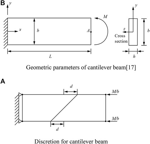
FIGURE 3. The cantilever beam with imposed to bending moment. (A) Discretion for cantilever beam. (B) Geometric parameters of cantilever beam (Yang et al., 2014).

In this case, the value which is calculated point $A$ is compared with the exact value which is $M{L}^2/\left(2E{I}_z\right)$ to illustrate the sensitivity of different numerical methods to the quality of the mesh. In Figure 4, the following conclusions can be obtained:

FIGURE 4

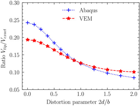
FIGURE 4. Curve of the ratio of calculated value to real value with twist parameter.

For the twist factor $2d/b$ is zero, the performance of FEM is better than VEM. With distortion parameters increasing, the accuracy of the FEM decreases faster than the VEM. The result of FEM is equal to VEM when the distortion parameter $2d/b$ is near 1. When the distortion parameter $2d/b$ exceeds 1, the accuracy of VEM is superior to that of FEM.

4.2 Example 2: Hertzian Problem

The second simulation is to testify the convergence rate and exactness of the algorithm. The reason for choosing the Hertzian contact as the second numerical example is an analytical solution to the Hertzian contact. The accuracy of the method is illustrated by comparing the computational and analytical solutions.

The model geometry is shown in Figure 5. The disc of the radius $R=10 m$ is loaded by a pressure $p=100Pa$. The $\mu =0.3$ and $E={10}^{3}Pa$ is selected as material parameters. Rectangular at the bottom of the model is taken as $L=20m,H=10 m,E={10}^{6}Pa,\mu =0.3$. The quadrilateral meshes are used. Because of the model’s symmetry, half of the models are selected for research.

FIGURE 5

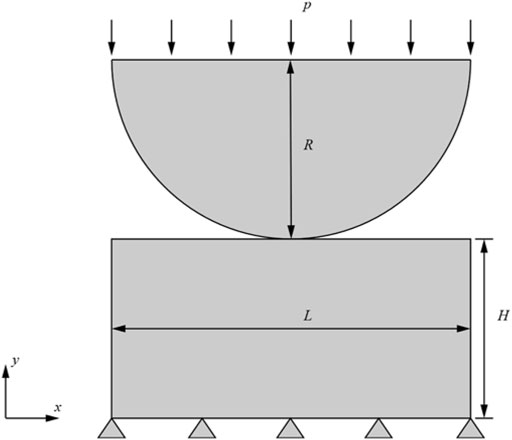
FIGURE 5. Hertz contact model.

It is known that the penalty factor has an impact on the result. When the number of mesh is 600, the number of iterations and the maximum contact force under different penalty functions are listed in the following Table1. From Table 1, the penalty factor is finally selected as ${\omega }_N^1=1\times {10}^4$. The model is discretized by 1,155 quadrilateral elements, as exhibited in Figure 6A. The contour of normal pressure is exhibited in Figure 6B.

TABLE 1

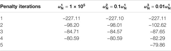
TABLE 1. The convergence process of penalty function for Hertzian contact.

FIGURE 6

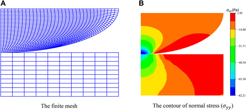
FIGURE 6. The finite mesh and contour of normal stress $\left({\sigma }_{yy}\right)$ is the normal stress in y-direction.

In Figure 7, the analytical solution, numerical solutions obtained by the VEM and the FEM for contact force are shown, respectively. Some conclusions can be drawn:

FIGURE 7

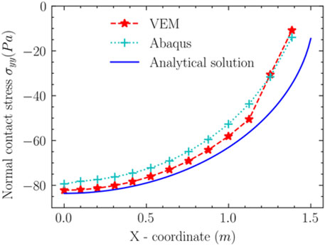
FIGURE 7. The normal contact stress distribution $\left({\sigma }_{yy}\right)$ along the contact zone.

In the contact region where $x$ is less than 1.4, the difference between the normal stress obtained by the VEM and the analytical solution is smaller than that obtained by the FEM. The maximum stresses of analytical solution, virtual element method, and FEM are 83.60, 82.21, and 80.57. When $x$ is more significant than 1.4, The curve of the VEM coincides with the FEM.

In practical problems, we are more concerned about the maximum normal contact traction. The contact stress with 389, 600, and 1,155 meshes are shown in Figure 8. There are some conclusions reached from Figure 9.

1) When the same mesh discretizes the structure, the maximum stress from the VEM is closer to the analytical solution.

2) The convergence rate of the VEM is higher than FEM for the number of the element from 389 to 600.

3) As the number of mesh elements increased from 600 to 1,155, the convergence rate of the VEM was the same as the FEM.

FIGURE 8

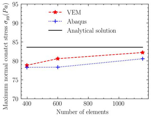
FIGURE 8. Maximum normal contact stress under different numbers of elements.

FIGURE 9

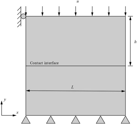
FIGURE 9. Model geometry with straight lines in the contact interface.

4.3 Example 3: A Horizontal Interface Under Uniform Compression

The third numerical model has been researched by Hirmand (Hirmand et al., 2015). This example is to compare the influence of different mesh shapes and the number of elements for contact stress. The geometry is shown in Figure 9. A displacement loads the upper rectangle in the y-direction $\left(u_y=-0.1 m\right)$. The displacements of the bottom of the model are both fixed. The Young’s modulus is $E={10}^9 Pa$. The Poisson’s ratio is $\mu =0.3$.

The advantage of VEM is to it calculates arbitrary mesh shapes. The Voronoi mesh (Talischi et al., 2012) is used to discrete the model. The normal stress along the contact interface of the different shape mesh with Hirmand is shown in Figure 10A. From Figure 10A, it can be concluded that the maximum normal contact stress is basically the same, with slight differences at both ends. Therefore, it can be noticed that the normal contact stress is slightly affected by the mesh shape. In this example, the influence of the different amounts of elements for the normal contact stress is studied. The 50, 100, 200, 300, and 500 Voronoi elements are employed to discrete the model. In Figure 10B, mesh 1, mesh 2, mesh 3, mesh 4, and mesh 5 correspond to 50, 100, 200, 300, and 500 Voronoi elements. Figure 10B presents the normal contact stress for different number elements. The following conclusions are obtained from Figure 10B: When the number of elements is 200, 300, and 500, the normal contact stress curves remain coincident.

FIGURE 10

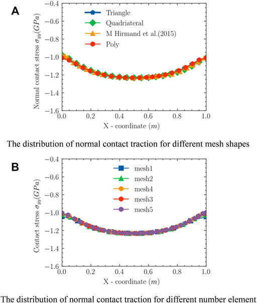
FIGURE 10. The distribution of normal contact traction in horizontal contact interface. (A) The distribution of normal contact traction for different mesh shapes. (B) The distribution of normal contact traction for different number element.

Figure 11A shows the contour of vertical displacement obtained by VEM under the Voronoi mesh. The simulation of Hirmand under quadrilateral mesh is presented in Figure 11B. It is noted that the curve for VEM is in line with the results shown by Hirmand. The contours of the normal stress $\left({\sigma }_{yy}\right)$ is shown in Figure 11C.

FIGURE 11

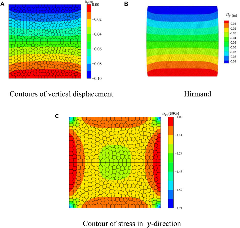
FIGURE 11. Contours of displacement and pressure for the $\text{vertical}$ direction (U_y is the displacement in y-direction and σ_yy is the stress in y-direction).

4.4 Example 4: Dam With Joint

This numerical example simulates a dam problem with a cracked foundation. This example is shown in Zheng (Zheng et al., 2002) in the 2005 year. The geometric model is exhibited in Figure 12A. The model size parameters are $L_1=25m$, $L_2=3m$, $L_3=2m$, $H_1=10m$, $H_2=5m$. The Young’s modulus $E={10}^{10}Pa$ and Poisson’s ratio $\mu =0.3$ are the material parameters for this model. The $\gamma =24kN/m^3$ is taken as volumetric weight. The displacements of the bottom left and right of the foundation are fixed. The coordinates of the joint tip are from (4,10) to (10,4). The joint end is fixed and will not propagate, and there is no friction at the crack interface.

FIGURE 12

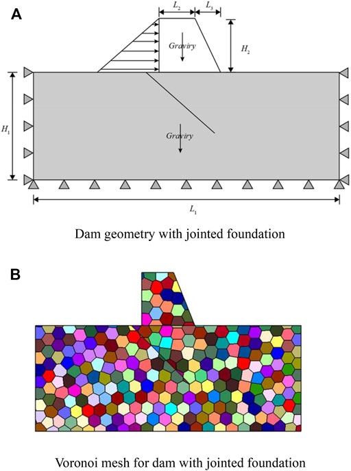
FIGURE 12. The geometric parameters and Voronoi mesh for dam with joint. (A) Dam geometry with jointed foundation. (B) Voronoi mesh for dam with jointed foundation.

The stress situation is analyzed using two load steps. The first load step only considers the self-weight of the dam body and foundation; the second load step applies a triangularly distributed normal water pressure to the surface of the dam body to simulate the condition of the reservoir after it is full of water. The Voronoi mesh was used to discretize the model. The Voronoi mesh is presented in Figure 12B. The displacement contour along the $x$-direction is demonstrated in Figure 13A, and the displacement contour in $y$-direction is shown in Figure 13B. From Figures 13A,B, it is noted that the displacement contours are discontinuous at the joint. The maximum and minimum principal stress contours are presented in Figure 14. As expected, the maximum stress occurs at the joint tip. The phenomenon is consistent with Li’s research (Li et al., 2022). In their studies, the strategy derived from the meshless numerical manifold method (MNMM) is employed by Li to solve linear elastic fractures.

FIGURE 13

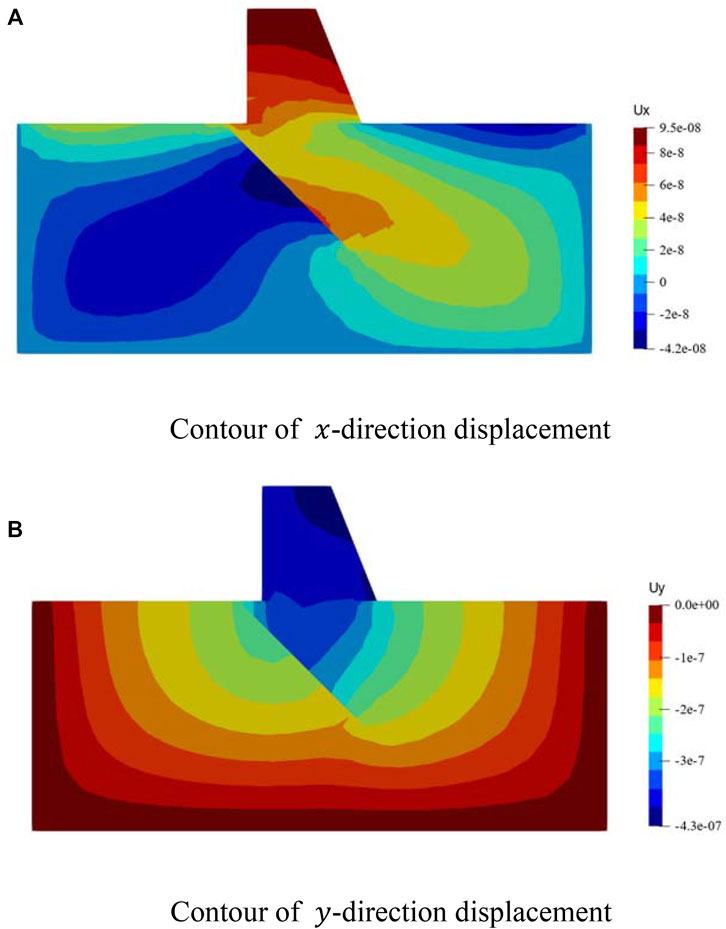
FIGURE 13. The contours of displacement in $x$ and $y$ directions (U_x and U_y are the displacement in displacement in x and y direction, respectively).

FIGURE 14

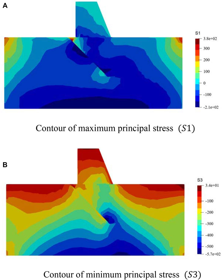
FIGURE 14. The contours of maximum principal stress $(S1$ is the maximum principal stress and minimum principal stress) $(S3$ is the minimum principal stress).

5 Discussion

In Example 1, when the distortion parameter is 0, the result of the FEM is more accurate than the VEM. The reason is that the function in the virtual element space satisfies the globally continuous on the element boundary. When the distortion parameter gradually increases, the downward trend of the resulting curve of the VEM is slower than that of the FEM. When the element distortion parameter exceeds a certain value, the result of the VEM is more accurate than the FEM. The result of VEM calculation is less affected by mesh quality.

In Figure 7 of example 2, the result of the VEM is better than the FEM in the contact region where $x$ is less than 1.4 because the discrete element size is small, which makes the element more twisted. And in the contact region where $x$ is more significant than 1.4, the main reason is that discrete element size is relatively large, so the element distortion is minor.

Under the 389 elements in Figure 8 of example 2, the main reason for the similar maximum normal stress of the VEM and the FEM is that the element distortion parameter is small. When the number of elements increases, the corresponding element size becomes smaller, the distortion increases, and the advantages of the VEM become more obvious. When the number of elements is 600, the difference between the VEM and the FEM results is greater than the difference between the VEM and the FEM when the amount of elements is 389. When the amount of elements is 1,155, the difference between the outcomes of the VEM and FEM is close to the difference between the outcomes of the amount of elements 600. On the whole, the better convergence and accuracy of the VEM in Hertz contact lies in the VEM is suitable for general polygons or polyhedrons, which is used flexibly for discrete complex contact surfaces (Beirão Da Veiga et al., 2013; Chen, 2015; Benedetto et al., 2016).

From example 1 and example 2, it can be known that the distortion of the element greatly influences the results. In example 3, normal contact stress in the contact interface is the same under different mesh shapes. The main reason is that the VEM test and trial space do not need to be accurately calculated, avoiding mesh dependence, and the contact interface is straight.

In example 4, a dam with cracks under Voronoi mesh was modeled. As expected, the maximum stress occurs at the joint tip in example 4, so the joint is an important cause affecting safety in engineering. So, the joint the focus of the study. Through example 4, it can be obtained that the NST contact model based on the virtual element method can solve engineering problems well under the Voronoi mesh.

6 Conclusion

A strategy to handle the contact problem is proposed in this paper, which is stemmed from the NTS model and the VEM. The effect of mesh distortion for results, the accuracy and convergence rate for Hertz contact, the impact of different mesh shapes and different elements numbers for results and the application of algorithms in engineering are implemented by several numerical examples. The results show that:

1) The VEM is insensitive to the mesh quality.

2) When the mesh on the contact interface is distorted, The VEM has high convergence and accuracy.

3) When contact problem is handled by VEM, the normal contact stress on the contact surface is slightly affected by the mesh shape.

4) The results in the fourth example show that the VEM can solve the contact problem in engineering under Voronoi mesh

Data Availability Statement

The raw data supporting the conclusion of this article will be made available by the authors, without undue reservation.

Author Contributions

YS performed the data analyses and wrote the manuscript. GS contributed significantly to analysis and manuscript preparation. QY and JW helped perform the analysis with constructive discussions.

Funding

Supported by the national Natural Science Foundation of China (Grant No. 11972043) and National Key R&D Program of China (2018YFE0100100).

Conflict of Interest

The authors declare that the research was conducted in the absence of any commercial or financial relationships that could be construed as a potential conflict of interest.

Publisher’s Note

All claims expressed in this article are solely those of the authors and do not necessarily represent those of their affiliated organizations, or those of the publisher, the editors and the reviewers. Any product that may be evaluated in this article, or claim that may be made by its manufacturer, is not guaranteed or endorsed by the publisher.

References

Béchet, É., Moës, N., and Wohlmuth, B. (2010). A Stable Lagrange Multiplier Space for Stiff Interface Conditions within the Extended Finite Element Method. Int. J. Numer. Methods Eng. 78, 931–954. doi:10.1002/nme.2515

CrossRef Full Text | Google Scholar

Beirão Da Veiga, L., Brezzi, F., Cangiani, A., Manzini, G., Marini, L. D., and Russo, A. (2013). Basic Principles of Virtual Element Methods. Math. Models Methods Appl. Sci. 23, 199–214. doi:10.1142/s0218202512500492

CrossRef Full Text | Google Scholar

Beirão da Veiga, L., Brezzi, F., Marini, L. D., Russo, A., Brezzi, F., and Manzini, G. (2014). The Hitchhiker's Guide to the Virtual Element Method. Math. Models Methods Appl. Sci. 24, 1541–1573. doi:10.1142/s021820251440003x

CrossRef Full Text | Google Scholar

Benedetto, M. F., Berrone, S., and Scialò, S. (2016). A Globally Conforming Method for Solving Flow in Discrete Fracture Networks Using the Virtual Element Method. Finite Elem. Anal. Des. 109, 23–36. doi:10.1016/j.finel.2015.10.003

CrossRef Full Text | Google Scholar

Chen, L. (2015). Equivalence of Weak Galerkin Methods and Virtual Element Methods for Elliptic Equations, 1–11.

Google Scholar

da Veiga, L. B., Lipnikov, K., and Manzini, G. (2014). The Mimetic Finite Difference Method for Elliptic Problems. Model. Simulation Appl. 11, 1–389. doi:10.1007/978-3-319-02663-3

CrossRef Full Text | Google Scholar

Flemisch, B., Puso, M. A., and Wohlmuth, B. I. (2005). A New Dual Mortar Method for Curved Interfaces: 2D Elasticity. Int. J. Numer. Meth. Engng 63, 813–832. doi:10.1002/nme.1300

CrossRef Full Text | Google Scholar

Hautefeuille, M., Annavarapu, C., and Dolbow, J. E. (2012). Robust Imposition of Dirichlet Boundary Conditions on Embedded Surfaces. Int. J. Numer. Methods Eng. 90, 1102–1119. doi:10.1002/nme.3306

CrossRef Full Text | Google Scholar

Hirmand, M., Vahab, M., and Khoei, A. R. (2015). An Augmented Lagrangian Contact Formulation for Frictional Discontinuities with the Extended Finite Element Method. Finite Elem. Anal. Des. 107, 28–43. doi:10.1016/j.finel.2015.08.003

CrossRef Full Text | Google Scholar

Hughes, T. J. R., Taylor, R. L., Sackman, J. L., Curnier, A., and Kanoknukulchai, W. (1976). A Finite Element Method for a Class of Contact-Impact Problems. Comp. Methods Appl. Mech. Eng. 8, 249–276. doi:10.1016/0045-7825(76)90018-9

CrossRef Full Text | Google Scholar

Khoei, A. R., Shamloo, A., and Azami, A. R. (2006). Extended Finite Element Method in Plasticity Forming of Powder Compaction with Contact Friction. Int. J. Sol. Structures 43, 5421–5448. doi:10.1016/j.ijsolstr.2005.11.008

CrossRef Full Text | Google Scholar

Krstulovic-Opara, L., Wriggers, P., and Korelc, J. (2002). A C 1 -continuous Formulation for 3D Finite Deformation Frictional Contact. Comput. Mech. 29, 27–42. doi:10.1007/s00466-002-0317-z

CrossRef Full Text | Google Scholar

Lee, N.-S., and Bathe, K.-J. (1993). Effects of Element Distortions on the Performance of Isoparametric Elements. Int. J. Numer. Meth. Engng. 36, 3553–3576. doi:10.1002/nme.1620362009

CrossRef Full Text | Google Scholar

Li, W., Yu, X., Lin, S., Qu, X., and Sun, X. (2022). A Numerical Integration Strategy of Meshless Numerical Manifold Method Based on Physical Cover and Applications to Linear Elastic Fractures. Eng. Anal. Boundary Elem. 134, 79–95. doi:10.1016/j.enganabound.2021.09.028

CrossRef Full Text | Google Scholar

Liu, F., and Borja, R. I. (2008). A Contact Algorithm for Frictional Crack Propagation with the Extended Finite Element Method. Int. J. Numer. Methods Eng. 76, 1489–1512. doi:10.1002/nme.2376

CrossRef Full Text | Google Scholar

Liu, F., and Borja, R. I. (2010). Finite Deformation Formulation for Embedded Frictional Crack with the Extended Finite Element Metho. Int. J. Numer. Methods Eng. 82, 773–804. doi:10.1002/nme.2782

CrossRef Full Text | Google Scholar

Liu, F., and Borja, R. I. (2010). Stabilized Low-Order Finite Elements for Frictional Contact with the Extended Finite Element Method. Comp. Methods Appl. Mech. Eng. 199, 2456–2471. doi:10.1016/j.cma.2010.03.030

CrossRef Full Text | Google Scholar

Liu, G. R., Dai, K. Y., and Nguyen, T. T. (2007). A Smoothed Finite Element Method for Mechanics Problems. Comput. Mech. 39, 859–877. doi:10.1007/s00466-006-0075-4

CrossRef Full Text | Google Scholar

Nguyen-Thanh, V. M., Zhuang, X., Nguyen-Xuan, H., Rabczuk, T., and Wriggers, P. (2018). A Virtual Element Method for 2D Linear Elastic Fracture Analysis. Comp. Methods Appl. Mech. Eng. 340, 366–395. doi:10.1016/j.cma.2018.05.021

CrossRef Full Text | Google Scholar

Ortiz-Bernardin, A., Russo, A., and Sukumar, N. (2017). Consistent and Stable Meshfree Galerkin Methods Using the Virtual Element Decomposition. Int. J. Numer. Methods Eng. 112, 655–684. doi:10.1002/nme.5519

CrossRef Full Text | Google Scholar

Padmanabhan, V., and Laursen, T. A. (2001). A Framework for Development of Surface Smoothing Procedures in Large Deformation Frictional Contact Analysis. Finite Elem. Anal. Des. 37, 173–198. doi:10.1016/s0168-874x(00)00029-9

CrossRef Full Text | Google Scholar

Remacle, J.-F., Lambrechts, J., Seny, B., Marchandise, E., Johnen, A., and Geuzainet, C. (2012). Blossom-Quad: A Non-uniform Quadrilateral Mesh Generator Using a Minimum-Cost Perfect-Matching Algorithm. Int. J. Numer. Meth. Engng 89, 1102–1119. doi:10.1002/nme.3279

CrossRef Full Text | Google Scholar

Sheng, Z., and Yuan, G. (2012). An Improved Monotone Finite Volume Scheme for Diffusion Equation on Polygonal Meshes. J. Comput. Phys. 231, 3739–3754. doi:10.1016/j.jcp.2012.01.015

CrossRef Full Text | Google Scholar

Stavroulakis, G. E. (2013). Lecture Notes in Applied and Computational Mechanics: Introduction.

Google Scholar

Sun, G., Lin, S., Zheng, H., Tan, Y., and Sui, T. (2020). The Virtual Element Method Strength Reduction Technique for the Stability Analysis of Stony Soil Slopes. Comput. Geotechnics 119, 103349. doi:10.1016/j.compgeo.2019.103349

CrossRef Full Text | Google Scholar

Sutton, O. J. (2017). The Virtual Element Method in 50 Lines of MATLAB. Numer. Algor 75, 1141–1159. doi:10.1007/s11075-016-0235-3

CrossRef Full Text | Google Scholar

Talischi, C., Paulino, G. H., Pereira, A., and Menezes, I. F. M. (2012). PolyMesher: A General-Purpose Mesh Generator for Polygonal Elements Written in Matlab. Struct. Multidisc Optim 45, 309–328. doi:10.1007/s00158-011-0706-z

CrossRef Full Text | Google Scholar

Wriggers, P., Krstulovic-Opara, L., and Korelc, J. (2001). Smooth C1-Interpolations for Two-Dimensional Frictional Contact Problems. Int. J. Numer. Meth. Engng. 51, 1469–1495. doi:10.1002/nme.227

CrossRef Full Text | Google Scholar

Yang, Y., Tang, X., and Zheng, H. (2014). A Three-Node Triangular Element with Continuous Nodal Stress. Comput. Structures 141, 46–58. doi:10.1016/j.compstruc.2014.05.001

CrossRef Full Text | Google Scholar

Yang, Y., Sun, G., Zheng, H., and Qi, Y. (2019). Investigation of the Sequential Excavation of a Soil-Rock-Mixture Slope Using the Numerical Manifold Method. Eng. Geology. 256, 93–109. doi:10.1016/j.enggeo.2019.05.005

CrossRef Full Text | Google Scholar

Yang, Y., Xu, D., Liu, F., and Zheng, H. (2020). Modeling the Entire Progressive Failure Process of Rock Slopes Using a Strength-Based Criterion. Comput. Geotechnics 126, 103726. doi:10.1016/j.compgeo.2020.103726

CrossRef Full Text | Google Scholar

Yang, Y., Sun, G., Zheng, H., and Yan, C. (2020). An Improved Numerical Manifold Method with Multiple Layers of Mathematical Cover Systems for the Stability Analysis of Soil-Rock-Mixture Slopes. Eng. Geology. 264, 105373. doi:10.1016/j.enggeo.2019.105373

CrossRef Full Text | Google Scholar

Yang, Y., Xia, Y., Zheng, H., and Liu, Z. (2021). Investigation of Rock Slope Stability Using a 3D Nonlinear Strength-Reduction Numerical Manifold Method. Eng. Geology. 292, 106285. doi:10.1016/j.enggeo.2021.106285

CrossRef Full Text | Google Scholar

Yang, Y., Wu, W., and Zheng, H. (2021). Stability Analysis of Slopes Using the Vector Sum Numerical Manifold Method. Bull. Eng. Geol. Environ. 80, 345–352. doi:10.1007/s10064-020-01903-x

CrossRef Full Text | Google Scholar

Zhang, B. R., and Rajendran, S. (2008). 'FE-Meshfree' QUAD4 Element for Free-Vibration Analysis. Comp. Methods Appl. Mech. Eng. 197, 3595–3604. doi:10.1016/j.cma.2008.02.012

CrossRef Full Text | Google Scholar

Zheng, H., Li, Z., Ge, X., and Yue, Z. (2002). Mixed Finite Element Method for Interface Problems. Chin. J. Rock Mech. Eng. 20, 1–8. doi:10.3321/j.issn:1000-6915.2002.01.001

CrossRef Full Text | Google Scholar

Zheng, H., Yang, Y., and Shi, G. (2019). Reformulation of Dynamic Crack Propagation Using the Numerical Manifold Method. Eng. Anal. Boundary Elem. 105, 279–295. doi:10.1016/j.enganabound.2019.04.023

CrossRef Full Text | Google Scholar