Amplification Behaviour of Compressional Waves in Unconsolidated Sediments

Similar to horizontal earthquake motions, vertical motions are amplified depedent on the local site conditions which can be critical for the safety of certain structures. Production of natural gas in Groningen, the Netherlands, results in reservoir compaction causing low magnitude, shallow earthquakes which are recorded with a borehole seismic network. These recordings form an excellent data set to understand how shallow unconsolidated subsurface geology influences the amplification behaviour of compressional waves (P-waves). First, we present borehole and single-station techniques (amplification factors, empirical transfer functions (ETF) and V/H spectral ratio implementations) to quantify vertical amplification. We show that vertical-wave incidence is a reasonable assumption. All techniques are capable of emphasising the sites with strong amplification of vertical ground motion during an earthquake. Subsequently, we compare ETF with single-station methods with the aim to develop proxies for vertical site-response using spectral ratios. In a second step, we link vertical site-response with shallow subsurface conditions, like the P-wave velocity and peat content. To better understand the amplification mechanisms, we analytically simulate P-wave propagation. In the simulations, we compute synthetic transfer functions using realistic subsurface conditions and make a comparison with the ETF. The simulations support the hypothesis that thin layers of shallow gas, originating from the Holocene peat, result in wave amplification. We observe strong vertical site-response in particular in the eastern part of Groningen, with industrial facilities and pipeline infrastructure in the region. Here, if high vertical amplifications are persistent at large earthquake magnitudes, appreciable levels of vertical loading may be expected. This study demonstrates that vertical motions should be assessed separately from horizontal motions, given that the amplification behaviour of P-waves is affected by distinctive mechanisms.

1 Introduction

Although the subsurface is subjected to earthquake shaking simultaneously in the horizontal and vertical directions, vertical motions have received less attention in ground motion studies than the horizontal counterpart. Primarily because it is generally assumed that the margins against gravity-induced static forces provide adequate resistance to dynamic forces induced by vertical ground motion. As a result, studies on the characteristics of vertical ground motion are limited in number, particularly at sites where the earthquake intensity is low. Many seismic design codes do not consider the vertical component of motion at all, or use a single scalar multiplication factor on the horizontal component of motion.

Newmark et al. (1973) suggest that the effect of the vertical response amplitude spectrum is typically represented as two-thirds of the horizontal spectrum. Subsequently, Eurocode 8 (CEN, 2004), propose a maximum vertical acceleration factor of 0.45, normalised over horizontal acceleration. In Eurocode 8 it is emphasised that vertical ground motion is not very much affected by the underlying ground conditions and hence no correction is made for possible amplification in shallow soils. However, analyses on multiple strong earthquakes (M$\ge 5$) have proven that vertical ground accelerations can exceed values of 2/3 of horizontal, especially at short periods and in near-source distance range. Hence, vertical motion should be treated separately from the horizontal component in ground-motion studies (Ambraseys and Simpson, 1996; Bommer et al., 2011; Bozorgnia and Campbell, 2016a,b; Elnashai and Papazoglou, 1997; Yang and Sato, 2000; Yang and Lee, 2007; Yang and Yan, 2009). In addition, Elgamal and He (2004) analysed borehole arrays across the world and observed amplification characteristics for compressional waves as for the shear-waves. Amplification mostly occurs in the top 20 m of the unconsolidated sediments but compressional waves have a different site-dependence. This means that vertical ground motion cannot be treated as a single-value fraction of horizontal ground motion but should be assessed independently.

Previously mentioned studies focus on high intensity earthquakes with a tectonic origin and relatively deep hypocentres. This paper investigates vertical ground motion for shallow (3 km), low magnitude (M_max = 3.6 thus far) earthquakes in Groningen, in the northeast of the Netherlands. Over the past decades, the extraction of natural gas from the Groningen gas field has triggered induced seismicity. Although the maximum magnitude of the local earthquakes is relatively low, the ground motions form a risk since the existing buildings and infrastructures are not built to withstand earthquake shaking. The Groningen shallow subsurface consists of low-velocity, unconsolidated sediments with strong site amplification which has been studied in detail for motions in the horizontal direction (Bommer J. J. et al., 2017; Rodriguez-Marek et al., 2017; van Ginkel et al., 2019, 2021). So far, it has been assumed that for these low-magnitude earthquakes, vertical ground motion is not of enough importance to incorporate into the ground motion model and in seismic design for buildings (Bommer J. et al., 2017). Neither have shake table tests (Kallioras et al., 2020) and building response modeling (Malomo et al., 2019; Korswagen et al., 2019), applied on Dutch structures, included vertical motions into their tests. However, in the Groningen area, the implosive component and the shallow nucleation depth of the induced seismicity results in relatively strong compressional waves (P-waves) (Dost et al., 2020). Moreover, specific near-surface geology could result in strong, and locally varying, P-wave amplification. Consequently, structures with large horizontal extent, such as bridges, pipelines or industrial facilities might suffer from a lateral difference in vertical motion from one end to the other. This can lead to stress within the structure and subsequently in failure (Saadeghvariri and Foutch, 1991).

The objective of this study is to qualify, and where possible quantify, vertical site-response based on local induced earthquake recordings in 69 borehole sites of the Groningen seismic network. For this network, we show that the amplification measured on the vertical component corresponds primarily to P-wave amplification. Site-effect related to the local geology is evaluated through an analysis of the spectral characteristics of both earthquake and ambient noise records. Subsequently, by comparing several seismic methods, we are able to develop single-station proxies for vertical site-response. Additionally, we perform 2D wave propagation simulations, in order to understand the effect of (sub-wavelength) subsurface conditions and angle of incidence of the earthquake waves.

2 Geological Setting

The province of Groningen, in the north-east of the Netherlands (Figure 2), is experiencing induced earthquakes due to the exploitation of a large onshore gas field. The Rotliegend sandstone reservoir is located at 3 km depth and is faulted during the Jurassic to Cretaceous rifting period. Here, reservoir compaction due to pressure depletion by the extraction of has reactivated the existing normal fault system that traverses the reservoir layer throughout the whole field Buijze et al. (2017).

The Groningen region has a flat topography and the groundwater table reaches almost up to the surface. The sedimentary cover is formed by the Cenozoic soft sediments, named the North Sea Group (NSG). In this study, we focus on the shallow subsurface, which is composed of unconsolidated Pleistocene sands and clays, overlain by a very heterogeneous Holocene formation (Figure 1). The Holocene formation is subdivided into several members. In Groningen, the Wormer and Walcheren Members mainly consist of marine clays, silt and fine sand. Two peat layers subdivide these two members. In the northern part, the Naaldwijk Formation mainly consists of sandy channel systems (MeijlesWong et al., 2007, 2015).

FIGURE 1

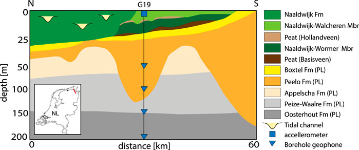
FIGURE 1. Schematic geological cross section of the upper 200 m of the soft sedimentary cover in the northeastern Groningen region (red line in inset). Note that the vertical scale is inflated for the top 50 m to highlight the stratigraphy of the Holocene formations on top of the Pleistocene (PL) formations. Borehole station G19 is featured because this site is used for wave-propagation modeling. The G-network vertical arrays consists 5 seismometers (accellerometer (blue square) at the surface and geophones (blue triangles) at depth) with a 50 m depth interval. This cross section is based on GeoTOP (www.dinoloket.nl).

3 Data Set

In order to monitor seismicity in the Groningen gas field, the Royal Netherlands Meteorological Institute (KNMI) deploys the Groningen shallow borehole network (Figure 2). This so called G-network spreads out over some 850 km² and consists of 69 stations (Dost et al., 2017), each station is equipped with three-component, 4.5 Hz geophones at 50 m depth intervals (50, 100, 150, 200 m) and an accelerometer at the surface. The stations are continuously recording since 2015 and the data is available via the data portal of Royal Netherlands Meteorological Institute (KNMI, 1993). In this paper we refer to “station” for the entire string with an accelerometer at the surface and four geophones at depth, and refer to “seismometer” for a single sensor measurement at a certain depth. Stations G15, G43, G53, and G68 are discarded from analysis due to malfunctioning of seismometers during a number of high magnitude earthquakes, hence not sufficient data is available.

FIGURE 2

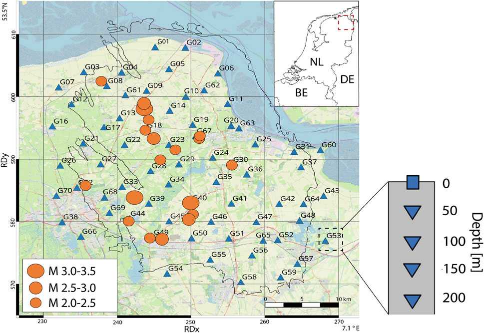
FIGURE 2. Map view of the Groningen borehole network in the northeast of the Netherlands. The triangles represent the surface location of each borehole site in the network. Each borehole contains an accelerometer at the surface and four 4.5 Hz geophones at depth with a 50 m depth spacing. The orange circles represent the local earthquakes with magnitude 2 or higher, recorded in the G-network between 05–2015 and 05–2019. Coordinates are shown within the Dutch National Triangulation Grid (Rijksdriehoekstelsel or RD) and lat/lon coordinates in the corners for international referencing. Background map: OpenStreetMap contributors, CC-BY-SA, www.openstreetmap.org.

The induced earthquakes recorded with the G-network have a magnitude of completeness of 0.5 (Dost et al., 2017). A maximum magnitude of 3.6 occurred during the Huizinge earthquake in 2012. Most earthquakes in Groningen have a normal faulting mechanism (Buijze et al., 2017; Dost et al., 2020).

4 Background

This chapter presents details on wave propagation to illustrate the assumption of near-vertical earthquake wave incidence in Groningen. Secondly, we present our definition of amplification based on reference conditions at depth.

4.1 Wave Propagation and Incidence

In this study we assess P-wave amplification behaviour by using local earthquake recordings of the vertical component of the Groningen borehole seismometers. For a straightforward analysis, we assume that the vertical component measures primarily P-waves. In this sections we show that this simplifying assumption largely holds.

Figure 3 shows a typical 3-component recording at the Earth’s surface in Groningen. P-waves are primarily recorded on the vertical component (Z), S-waves map primarily to the radial (R) and transverse (T) components. The well separation in wave types is largely due to the low near-surface velocities and hence small angles of incidence. In the top 200°m, P-wave velocities range, for most sites, between 1 and 2 km/s (Hofman et al., 2017). At close range to the epicenter, angles of incidence are close to zero. At larger range, P-waves have apparent horizontal propagation velocities of approximately 5.1 km/s (Jagt et al., 2017) resulting in angles of incidence varying between 11 and 23° in the top 200 m. Similar values are empirically found by Hofman et al. (2017). These angles of incidence results in 86–96% of the P-wave mapping to the vertical component. For S-waves, angles of incidence are even smaller in the near-surface due to very low velocities, down to about 35 m/s (Zwanenburg et al., 2020). And hence, not much S-wave energy can be recorded on the vertical component, as can be seen in Figure 3.

FIGURE 3

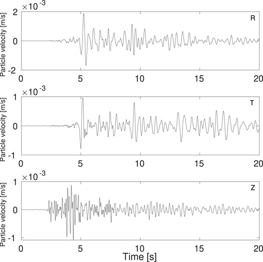
FIGURE 3. 3-component seismogram recorded at the surface station of borehole G62 for the 08–01–2018 M3.4 Zeerijp earthquake. R = radial/east component, T = transverse/north component, Z = vertical component.

Further details of the near-surface propagation can be seen at Figure 4. In panel 1) the amplification can be noted when comparing the signal recorded at 200 m depth and at the surface. It can be seen that most of this amplification occurs in the top 50°m. The particle motion on the radial-vertical plane is presented in Figures 4B,C. The time window (0–4 s) around the first P-arrival shows that this arrival primarily oscillates in the vertical direction. The time window (5–9 s) around the first S-wave arrival, on the other hand, shows it has a near-horizontal polarization. P-S and S-P conversions do occur in the near-surface, but are small in size, again due to the small angles of incidence. In 4) and 5) the difference in Fourier Amplitude Spectra (FAS) are shown for the 200 m and surface levels. The FAS illustrate that the largest amplitudes reside between 2 and 10 Hz.

FIGURE 4

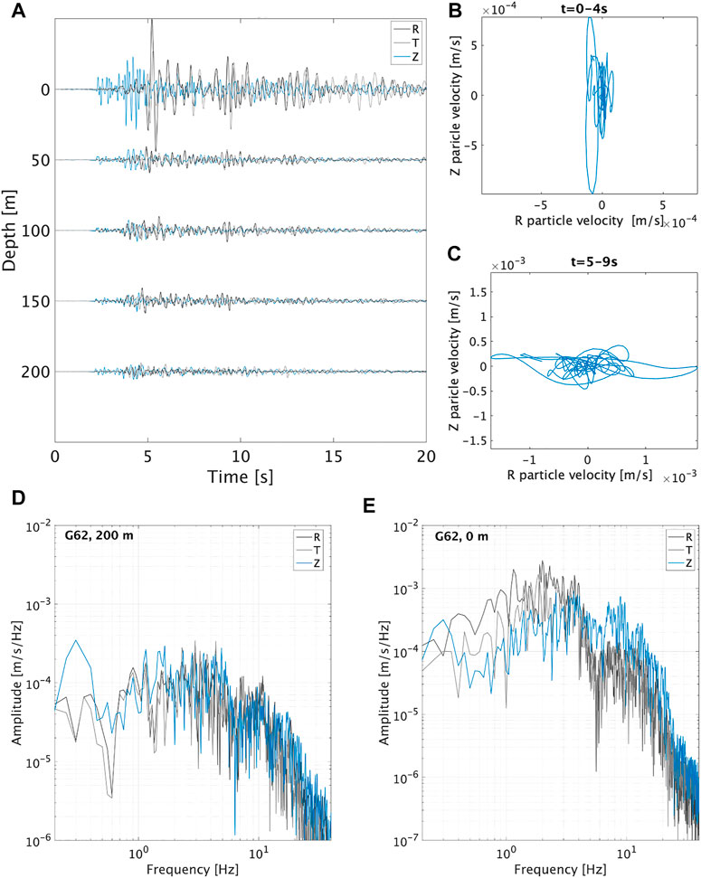
FIGURE 4. Earthquake record in particle velocity for station G62 for the Zeerijp earthquake on January 2018 with magnitude 3.4 for a 20 s window after earthquake origin time. With in panel (A) 3-component borehole seismogram. (B) Particle motion in the R-Z plane for the direct P-wave arrival for a time window of 0–4 s for G62 surface seismometer. (C) Particle motion in the R-Z plane for the direct S-wave arrival for a time window of 5–9 s for G62 surface seismometer. (D) Fourier Amplitude Spectra of the 200 m seismometer. (E) Fourier Amplitude Spectra of the surface seismometer.

Therefore, also from an engineering point of view, processing of the raw earthquake records was performed in the frequency band of 1–10 Hz. This study uses the three-component data set of 19 earthquake recordings from local events with magnitude two or higher. Earthquakes in this magnitude range have sufficient energy to be recorded in the entire network and are therefore usable for assessing site-response. The FAS includes source, path and site-effect. Site-effects are extracted by taking spectral ratio’s and or averaging over earthquakes with different hypocentres (and thus different source and path effects).

Further details on propagation from source to surface can be deduced from finite-difference simulations. The supplementary material contains the details of the model setup and input data for this simulation. Figure 5 shows the seismic wave field in the subsurface originating moderate-size earthquakes at reservoir depth (3 km), mimicing a limited shear rupture in a fault plane. The figure shows three snapshots of the vertical (Z-component) and horizontal (R-component) particle velocities after the start of the event. The shape of seismic wave fronts deforms to almost horizontal when they reach the shallow subsurface. Hence, a borehole geophone near the epicentre measures mainly P-waves on the sensor for the vertical particle velocity. The waveform simulations support the observations from the earthquake recordings as presented in Figure 4 and the assumption of almost vertical P-waves.

FIGURE 5

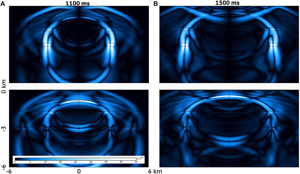
FIGURE 5. 2D full wave form finite difference model snapshots of absolute vertical (top) and horizontal (bottom) particle velocity for (A) 1100 ms after start of the earthquake, (B) 1500 ms. All panels have the same distance and particle velocity scale as the panel in the bottom left. The used velocity model is shown in Supplementary Figure S1.

The following analyses of earthquake wave propagation includes time windows of 20°s after earthquake rupture, and comprises not just the first P-wave arrival time window as presented in Figure 4B. We deliberately choose this extended time window because in the frequency domain, the signal becomes more stable by including complex body-wave reverberations of the earthquake coda wave window. These complex arrivals experience similar amplification between 200°m depth and the surface.

4.2 Ground Motion Amplification in Groningen

In the Groningen region, S-wave ground motion amplification is mainly governed by two factors; firstly the reduction in seismic velocities with decreasing depth and secondly, the presence of a velocity contrast at a certain depth causing resonance in the near-surface layer (van Ginkel et al., 2019). If this resonance of this near-surface layer has a similar resonance frequency as the structures at the surface, hazardous shaking can develop. In addition, shaking will not only occur at a single fundamental frequency but also at overtones. Amplification of P-waves follows the same physics as for S-waves, but has a different susceptibility to the near-surface lithology. Firstly, as P-waves have longer wavelengths, a deeper portion of the near-surface zone is relevant for resonance. Secondly, different impedance contrasts might be important, e.g., the interface between a water-saturated clay and sand has a high S-wave, but a low P-wave impedance contrast.

The example borehole seismograms and the FAS (Figure 4) show a major increase in amplitudes between the vertical component of the 200 m depth and the surface seismometer. Here, local site amplification occurs, on top of the free-surface effect. This amplification in the top 200 m is observed in multiple seismograms across the Groningen network.

Generally, amplification is quantified with respect to a hard rock outcrop over a full spectrum, however, these measurements are lacking in Groningen due to the 800–1,000 m thick sediment cover over the entire area. Alternatively, we define a reference site as a hypothetical outcrop with P-wave velocity of 1,900 m/s and a density of 2040 kg/m³. These are the values that are found, on average, in Groningen at 200 m depth (Romijn, 2017; Hofman et al., 2017).

5 Methodology

Amplification defined in the frequency-domain uses the Fourier Amplitude Spectra (FAS) of the earthquake records. The FAS (U_ij(f)), for the ith event and jth station, can be written as a convolution (i.e., multiplication in the frequency domain) of a source, path, site-effect and instrument term:

$U_{ij}\left(f\right)=S_i\left(f\right)G_{ij}\left(f\right)L_j\left(f\right)I_j\left(f\right),(1)$

where S_i is the source term, G_ij is the path term (between the ith event and the jth station), L_j is the site term, and I_j is the instrument-response term. I_j is known and removed before further processing the data. This leaves the source, path and site terms. Different approaches are used to extract from this the site term.

5.1 Empirical Transfer Functions

Quantification of site-effects across a frequency range of 1–10 Hz is performed by calculating borehole empirical transfer functions from local earthquake recordings. As shown in the previous section, we assume that vertical component is comprised of mainly P-waves in the 20 s time window used for the earthquake data processing. Therefore, the empirical transfer functions (T_m,n) represent P-wave amplification and are defined as a division of the Fourier amplitude spectra at two different depth levels

$T_{m,n}\left(f\right)=\frac{U_m}{U_n},(2)$

where m is the depth level of interest and n the reference horizon (Liu and Tsai, 2018; Rong et al., 2019). In U_m and U_n the source and path terms (Eq. 1) are (nearly) identical and hence the transfer function is only a description of the local propagation effects. When U_m is chosen at the Earth’s surface, T_m,n describes site-effects and |T_m,n| describes the frequency-dependent amplification with respect to the reference horizon.

In order to further improve estimation of the site-effect, we average the deconvolution (Equation 2) over 19 events with magnitudes $>$ 2.0. This can be seen as an implementation of seismic interferometry by deconvolution (Wapenaar et al., 2010). We use 20 s long time windows for particle velocity recordings on the vertical component of the borehole stations. In this implementation, for each event the deconvolution is applied as in Equation 2. Subsequently, the deconvolution results are stacked to enhance stationary contributions. With a reference horizon at 200 m depth and the level of interest at the Earth’s surface, the transfer function has both a causal and acausal part. The causal part maps upward-propagating waves, from the reference level to the surface. The acausal part maps downward-propagating waves back to the free surface (Nakata et al., 2013). To describe amplification, we are only interested in the causal part. We select this causal part of the estimated transfer function and compute its Fourier amplitude spectrum to obtain a measure of frequency-dependent amplification. The resulting amplitude spectrum we call the empirical transfer function (ETF). In order to get an estimate of uncertainty in the results, the above processing sequence is applied per earthquake and the standard deviation is computed from the resulting distribution.

5.2 V/H Spectral Ratios

Instead of the frequently used Horizontal-to-Vertical Spectral Ratio (HVSR) to estimate site-effects, we explore the option of using the inverse of the HVSR, the vertical-to-horizontal spectral ratio (VHSR). The HVSR-method (Nakamura, 1989, 2019) is based on the assumption that the vertical component spectrum is quite flat, hence a peak in the spectral ratios is generated by a peak in the horizontal component spectrum, which would be related to S-wave resonance. However, the spectrum of the vertical component is not flat, as demonstrated in the previous sections and supported by the findings of Sarmadi et al. (2021). By taking the inverse of HVSR, we can also not assume that the horizontal component spectrum is flat. However, peaks and troughs related to P-wave resonance and S-wave resonance are generally well separated in frequency. Comparing the spatial distribution between amplification established by the ETF and the one obtained with the VHSR, makes it possible to assess whether the VHSR can be used as tool to act as a proxy for P-wave amplification. Also, Lermo and Chavez-Garcia (1993) uses the VHSR to estimate resonance frequencies and peak amplitudes for the vertical component of ground motion from local earthquake recordings.

From earthquake recordings, generally time windows are picked containing direct arrivals of seismic waves to calculate the HVSR for site-response estimations (Chin and Aki, 1991; Mayeda et al., 1991; Kato et al., 1995; Su et al., 1996; Bonilla et al., 1997; Sánchez-Sesma et al., 2011). However, given that the local earthquakes are shallow and at short range, the window of the direct arrivals is very short, hence this implementation of VHSR is unstable. As alternative we use the coda window, which includes reverberations of the P-and S arrivals and reveals information on the local structure. Perron et al. (2018) evaluate the standard spectral ratio curves of the direct S and P-arrivals and the coda wave window and show that both parts of the waveform provide similar results. The signal must be of long enough duration to include sufficient reverberations to produce any resonance peak. The longer the picked window, the more back-scattered waves coming from many azimuths (illustrated in Figure 5) are included in the signal, resulting in a directionally averaged site-effect. By taking the ratio of the vertical and horizontal components, the propagation effects included in the signal largely vanish. Data processing for obtaining the VHSR from local event recordings is carried out in the following steps:

• Application of bandpass filter on earthquake recordings of 1–10 Hz

• Selection of a 15 s coda window, starting at (hypocentral distance/mean Vs.) + 5 s after earthquake origin time.

• Check whether the local earthquakes have a sufficient signal-to-noise ratio for the selected coda wave time window

• From the coda wave window, calculation of VHSR from power spectral densities (PSDs). Following (the reciprocal of) the procedure described in van Ginkel et al. (2020), the VHSR is computed from the vertical component (Z) and horizontal components (E and N) as:

$VHSR=\frac{\sqrt{PS{D}_Z}}{\sqrt{PS{D}_E+PS{D}_N}},(3)$

where the horizontal components are averaged by vector summation.

• Per site, averaging of the VHSR curves (by stacking in the frequency domain) over all local events. Figures 9A–F shows examples.

• Picking the peak amplitude for each averaged VHSR curve

6 Results and Interpretation

6.1 Amplification Factors

We calculate an overall amplification factor in the range of 1–10 Hz over the borehole vertical array, following the procedure described in van Ginkel et al. (2019, 2021). The AF is computed for each borehole site by taking the ratio of the maximum amplitudes recorded within 20 s after rupture time at the vertical component of the surface and the 200 m deep seismometer. The amplitude at the surface was divided by a factor of 2 in order to remove the effect of free surface amplification. Next, the AF per borehole is obtained by repeating the above procedure for all available M$>$ 2.0 events and subsequently averaging the values. A signal-to-noise threshold is applied on the events.

Throughout the borehole network, a maximum AF of 2.7 is reached at the eastern edge of the network, while other locations do not experience P-wave amplification at all (Figure 6). Hence, this AF-plot presents a first indication of the spatial variability across the G-network of vertical ground-motion amplification. Amplification factors from records on the horizontal components are calculated by van Ginkel et al. (Figure 4; 2019) and display a different spatial pattern than the vertical AFs, which is further investigated in the following sections.

FIGURE 6

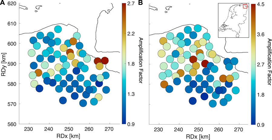
FIGURE 6. (A) Spatial distribution of the amplification factors computed based on earthquake records on the vertical component of the borehole seismometer at 200 m and at the surface. (B) Spatial distribution of the amplification factors computed based on earthquake records on the horizontal components of the borehole seismometer at 200 m and at the surface, modified from van Ginkel et al. (2019).

6.2 Empirical Transfer Functions

In order to get an estimate of uncertainty, the above processing sequence is applied per event and from the resulting distribution, the standard deviation is computed and examples are plotted in Figure 7A–F. For these examples, also the ETF between 200 and 50 m depth is shown. It can be seen that most of the amplification occurs in the top 50 m.

FIGURE 7

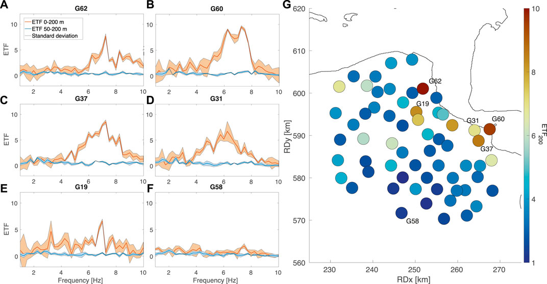
FIGURE 7. (A) Each panel depicts the empirical transfer functions (ETFs) between the seismometer at 200 m depth and the surface (red) and standard deviation (pale red area) for sites G19, G31, G37, G60, and G62, displaying the frequency-dependent amplification. The blue lines illustrate the ETFs between the seismometers at 200 m and 50 m. Borehole G62 additionally depicts the ETF between the surface and 50 m seismometer (gray). Borehole G58 is added as example of a borehole site with no amplification measured. (B) Spatial distribution of the peak amplitudes from the ETF for 60 borehole station sites.

Some ETFs show multiple side peaks, but the peak with largest amplitude value is identified as resonance peak, following the recommendation by Zhu et al. (2020). At some sites, this resonance peak has a large contribution to the overall amplification. Applying smoothing on the FAS and ETF can lead to suppression and shifting of peaks. We apply no smoothing and pick the largest amplitude and corresponding frequency. G58 has been added to Figure 7F to illustrate an ETF for a site with no amplification of P-waves. For 60 borehole stations, the ETF is computed. Subsequently, for each site, the corresponding peak amplitude for the 200 m -interval ETF is identified. Figure 7G depicts the spatial distribution of these peak amplitudes. Here, the distribution of amplitudes shows highest values in the eastern section of the region.

6.3 V/H From Spectral Acceleration

The previous section describes maximum amplification across a frequency range using the Fourier amplitude spectra of earthquake recordings of the borehole seismometers. However, Kramer. (1996) and Eurocode 8 (CEN, 2004) suggest using spectral ordinates at a varying range of periods in the acceleration response spectrum as ground-motion parameter.

As input, earthquake recordings (20 s after earthquake origin time) at the surface are taken to calculate the pseudo spectral acceleration (PSA). Subsequently response spectra (Figure 8A) for all three components, for each surface seismometer site, are calculated for pre-defined spectral periods (0.01–5.0 s), and taking the standard critical damping factor of 5% (Kramer, 1996; CEN et al., 2004). Per a defined period and per event, a V/H ratio is calculated from the PSA by dividing the vertical PSA with the geometric mean of the horizontal components. Subsequently, for each pre-defined period, an average V/H is calculated over all events and plotted in Figure 8B. As shown in 8b, in Groningen the V/H PSA value for certain locations at short periods is exceeding the standard values of 0.45 and 2/3 by Eurocode 8 and ASCE. Moreover, it is shown that for each period, there is a vast range of site-specific V/H PSA values. At long periods (T$>0.3$ s) the average value becomes closer to the single values proposed in literature. At short periods (T$<0.3$ s) the average is considerably higher (0.81 for T = 0.1 s).

FIGURE 8

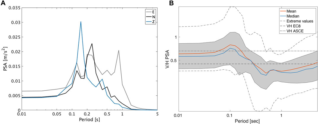
FIGURE 8. (A) Example of acceleration response spectrum for the surface seismometer at station G60 from the Westerwijtwerd earthquake of M = 3.4, where the blue line represents the PSA at the vertical component, the gray line the eastern horizontal component and in black the northern horizontal component. (B) Averaged V/H from response spectra for each surface seismometer, processing 20 earthquake recordings, at each defined period plotted together with the mean (red) and median (blue) and extreme values (dashed gray) per period. The shaded area depicts the mean plus-minus one standard deviation, the black dashed line illustrates the 0.45 value as proposed by Eurocode 8 and the dot-dash the 2/3 value proposed by the ASCE.

6.4 V/H Spectral Ratios

In this section we assess an additional single-station method for characterizing the spatial distribution of P-wave amplification. In Groningen, the induced events do not include surface waves at the short ranges within the G-network. The coda-based VSHR is therefore primarily a spectral ratio of P- and S-wave reverberations in the unconsolidated sediments. At many sites in Groningen, VSHR curves reach levels above 1 for distinct frequencies (Figure 9A). Location G58 is added as reference illustrating a VHSR below 1; here the horizontal component is dominating over the vertical for all presented frequencies. Figure 9A is illustrating the spatial distribution of VHSR peak amplitudes across the Groningen area.

FIGURE 9

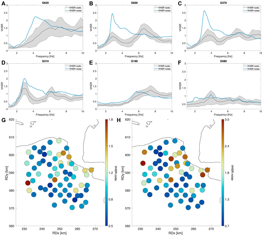
FIGURE 9. (A–F) Each panel depicts the mean VHSR (black line) and standard deviation (dashed line) for the surface seismometer for the stations G19, G31, G37, G60, G62, where high VHSR amplitudes are calculated. Station G58 is added as reference to show a VHSR for a location with no amplification of P-waves. The blue line indicates the VHSR from the ambient noise field. (G) Spatial distribution of coda-based VHSR peak amplitudes for each surface seismometer in the Groningen network. (H) Spatial distribution of noise-based VHSR peak amplitudes for each surface seismometer in the Groningen network.

6.4.1 VHSR From the Ambient Seismic Field

Site-effects are commonly assessed by using the ambient seismic noise field, (e.g., Bonnefoy-Claudet et al. (2006)). In Groningen, the noise level is sufficiently high in order to exceed the sensitivity of the surface accelerometers (Koymans et al., 2021). In addition to coda VHSR, the VHSR is also estimated from 1 month of ambient noise field measurements (VHSR_ASF), using the approach presented in van Ginkel et al. (2020, 2019).

In Figures 9A–F, the mean VHSR_ASF curves are added in blue for comparison with the VHSR_coda curve characteristics in order to investigate whether noise can be used as a proxy for site amplification. From the VHSR curves, the corresponding peak amplitudes are determined for each surface seismometer in the Groningen network. In general, the noise-based VHSR peak amplitudes are larger than the coda-based VHSR peak amplitudes. This is a common observation, and is most likely caused by the strong presence of surface waves in the noise. The surface-wave ellipticity has notches which inflate the amplitude levels of VHSR (Bonnefoy-Claudet et al., 2006; Konno and Ohmachi, 1998). Figures 9G,H presents the peak amplitudes from coda-based and noise-based VHSR, for each surface seismometers in the Groningen network. The spatial distribution of amplitudes exhibits a comparable pattern for both types of VHSR.

6.5 Relationship With Subsurface Conditions

The AF, ETF and V/H ratio peak amplitude distribution demonstrate a consistent pattern of increased peak amplitudes measured in the eastern part of the Groningen region (Figures 6, 7, 9). In order to understand this large variation in amplification, this section elaborates on the effect of shallow subsurface conditions on amplification behaviour of P-waves.

6.5.1 Seismic Velocities

Wave amplification is largely determined by local variations in seismic velocities. For each borehole location, P-wave interval velocities are known for the upper 200 m, with a 50 m interval resolution (Hofman et al., 2017). These velocities were computed by applying seismic interferometry to events recorded within the borehole stations. Since the majority of the peak amplitude increase arises in the top 50 m, the ETF peak amplitudes (Section 6.2) are plotted against the average P-wave velocities Vp for the top 50 m (Figure 10A). All strong amplifications (high ETF peak amplitudes) occur at velocities below 1,400 m/s. The relation between the near-surface P-wave velocity and the maximum amplification from the ETF is fitted (Rsq = 0.52) by an exponentially decaying function (Eq. 4). This empirical relation can be used to estimate the maximum amplification A in the vertical direction at other sites with unconsolidated sediments, when the average velocity Vp over the top 50 m is known:

$A=2.4+114e^{-0.004Vp}(4)$

FIGURE 10

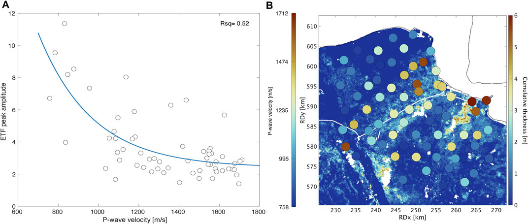
FIGURE 10. (A) Correlation between P-wave velocities for the top 50 m and ETF peak amplitudes, fitted with an exponential decaying function (Eq. 4). (B) Spatial distribution of the P-wave velocity values (Hofman et al., 2017) for the top 50 m for each borehole location (circles) plotted on top of the cumulative thickness map of Holocene peat.

Next, the interval P-wave velocity distribution is compared to the shallow lithostratigraphy throughout Groningen. For this purpose, cumulative thickness maps for different lithologies are extracted from the digital geological model GeoTOP (Stafleu et al. (2011; 2021), www.dinoloket.nl). The P-wave velocity distribution satisfactorily corresponds to areas with accumulations of peat in the shallow subsurface (10b). Thus, peat accumulations correlate with relatively low interval P-wave velocities. As a consequence, high ETF peak amplification develops during an earthquake where peat accumulates.

6.5.2 Effect of Gas on P-Wave Velocity

Since peat originates from organic material, methane can be generated, stored or migrated upwards and subsequently being trapped in the overlying sediments during burial. Although the peat layers are relatively thin in the Groningen field (less than 1 and up to 6 m throughout the top 50 m), their presence and resulting gas content can significantly reduce the P-wave velocity V_p [m/s]. The effect of gas on V_p can be understood from the Biot-Gassmann equations for wave propagation in poro-elastic media, such as soil Biot (1962) or Fjaer et al. (2008). Take that for seismic frequencies the so-called undrained condition holds and that the relative fluid displacement with respect to the rock can be neglected. In this case, $V_p=\sqrt{K^{″}/\rho }$ where ρ [kg/m³] is the bulk density and K″ = K + α²M + 4G/3 [Pa] where K and G [Pa] are the bulk and shear moduli of the drained rock and α = 1 − K/K_s [-] is the so-called Biot constant. K_s [Pa] is the bulk modulus of the grains in the rock. M [Pa] is a poro-elastic constant which can be expressed as:

$M=\frac{K}{\left(1-\alpha \right)\alpha -\varphi \left(1-\alpha -K/K_f\right)}(5)$

Where ϕ [m³/m³] is the pore volume fraction and K_f [Pa] is the effective bulk modulus of the fluid. For a fluid containing both gas and water at equal pressure, 1/K_f = S_w/K_fw + (1 − S_w)/K_fn. S_w [m³/m³] is the volume fraction of pore water or the water saturation. K_fw and K_fn[Pa] are the bulk moduli of water and gas. In the shallow subsurface, K_fn ≪ K_fw. Even for very low gas saturations, K_f ≈ S_n/K_fn. Further, K ≪ K_s at least for clay and sand. So this implies, α ≈ 1 and M ≈ K_f/ϕ ≈ S_n/(ϕK_fn). Since unconsolidated soil has a reasonable porosity, K″ ≈ K + 4G/3. So, the fluid stiffness hardly contributes to the stiffness of the rock and K″ approximates the so-called drained bulk modulus of soil. A direct consequence is that V_p values for peat at shallow depth can be become quite low. Values in the range 0.2–0.5 km/s are possible as has been measured by Mad Said et al. (2015); Zimmer et al. (2007). In the following we show the effect of low V_p-layers in the shallow subsurface on P-wave amplification by computing theoretical transfer functions (TTFs) from 2D wave propagation simulations. As has been shown in Section 4.1, at the near surface, the incoming waves have a maximum angle of incidence of 23°. Hence, simulations have been done for 0, 10 and 20° angles of incidence.

6.6 Shallow 2D Wave Propagation Simulations

From 2D wave propagation simulations in the shallow subsurface, we calculate the impact of subsurface lithology on P-wave amplification. Details on the simulations like the velocity and damping profiles, and the model setup are presented in the Supplementary Material. The effect of gas saturated layers in the shallow subsurface is implicitly included in the choice of the V_p profiles. In particular, we have selected the lithology around borehole location G19 in the Groningen field where the ETF displays high peak amplitudes for frequencies around 6, 7 Hz. Instead of 1D simulations, we deliberately performed 2D simulations to understand also the effect of the angle of incidence on wave amplification and on P-to-S wave conversion. Moreover, we compared the empirically-derived ETFs with the synthetic or theoretical ones (TTFs) from the simulations. The supplementary material presents the simulation details, the input data and model set up (Supplementary Section 1.2).

6.6.1 Theoretical Transfer Functions

The theoretical transfer functions (TTF) are calculated from P-wave displacement velocities recorded at the vertical component of probe 1 at the surface and probe 2 at 200 m depth (Supplementary Figure S3). Since the shallow P-wave velocity profile is hypothetical (Supplementary Section 1.2) first a sensitivity analysis of the TTF on the P-wave velocity profile in performed (Figures 11A,B). For both profiles, the TTFs for various angles of incidence (θ = 0, 10 and 20°) exhibit similar characteristics in terms of peak frequencies and amplitudes. Furthermore, Figure 11A shows that the effect of the wave front incidence angle is minor on the TTF curve characteristics. Higher angles of incidence shift the TTF peak frequency from 6.6 to 6.9 Hz as the travel time of the wave between the probe locations reduces.

FIGURE 11

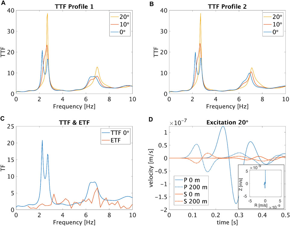
FIGURE 11. (A) Theoretical transfer functions (TTF) for P-wave velocity Profile 1 for various angles of incidence. (B) TTF for P-wave velocity Profile 2 for various angles of incidence. (C) Theoretical (blue) and empirical (red) transfer function for borehole G19. (D) Excitation (in velocity) for the P-waves on the vertical plane (blue) and S-waves on the horizontal plane (red) at 200 m (dashed) and at the surface (solid) with θ of 20°. The inset depicts the related particle motion at surface for the P-wave arrival time window.

Figure 11C compares the ETF with the TTF for velocity Profile 1 for zero angle of incidence (θ = 0°). Both transfer functions have a peak between 6 and 8 Hz, which peak is related to near-surface amplification. Between 2 and 3 Hz, the character of the transfer functions is quite different. The TTF peak around 2.5 Hz develops due to a notch at the 200 m recording. This notch is caused by the interference of up- and down-going waves. In the simulations, the subsurface is assumed laterally uniform. In reality, the subsurface is laterally quite heterogeneous, suppressing or disrupting such a notch. As a result, the ETF has no strong peak around 2.5 Hz. Moreover, the TTF is based on the propagation of a single wavelet while the ETF is an average from multiple earthquakes with various angles of incidence and azimuths. With this simulated transfer functions, we show that a varying angle of incidence is not of major influence on the amplification behaviour of P-waves.

6.6.2 P-To-S Wave Conversion

For non-zero angles of incidence on a layer interface, P-to-S wave conversion occurs. This conversion is of practical importance since prior to the direct S-wave arrival, P-waves might convert to S-waves and extend the period of exposure of buildings to horizontal ground motions during an earthquake. For the simulated small angles of incidence a limited P-to-S wave conversion can be seen in Figure 11D. It shows the simulated vertical P-wave and horizontal S-wave displacement velocities at 200 m and at the surface for a wave front with an angle of incidence of 20°. At around 0.23 s, when the high amplitude P-wave arrives at the surface, only minor S-wave excitation develops. Additionally, the particle motion plot (inset) for this time window comprises mainly a motion in the vertical (Z) plane. Since the generated S-wave amplitudes remain only a fraction of the P-wave amplitudes (less than 20%), this P-to-S wave conversion is deemed unimportant for the amplification and duration of the ground motion.

7 Discussion

This paper presents various empirical methods for the qualification of site-effects on vertical ground motion amplification of signals originating from induced earthquakes for the Groningen gas field. In characterising amplification in the vertical direction, we used 1) amplification factors, 2) borehole transfer functions, 3) V/H from spectral accelerations, and 4) V/H spectral ratio’s from earthquake coda-waves and the ambient seismic field. All four approaches exhibit a similar distribution of the degree of amplification in the vertical direction for each borehole site. In a second step, we explain this site-dependent amplification distribution depending upon the shallow subsurface composition and perform simulations in order to model the effect of low-velocity peat layers on P-wave propagation. In the following paragraphs we discuss the validity, uncertainties and the approaches presented, as well as the limitations.

Throughout this study we assume P-wave dominated vertical motions due to nearly vertical incidence of the seismic waves, hence the absence of direct wave type conversions. The following arguments show the validity of the previous hypothesis: 1) the range of angles of incidence (0–20°) is small and 2) empirical as well as theoretical particle motion plots mainly show motion in the vertical plane within the P-wave arrival time window. These criteria lead to an expectation we measure predominantly P-waves.

To test the influence of non-zero incidence, we varied the angle of incidence in the synthetic 2D wave propagation simulations. As shown in Figure 11D, varying the angle of incidence of the wave front does not lead to major P-to-S-wave conversions. Therefore, we consider the assumption that the vertical component represents the amplification of the P-waves as valid.

Previous studies (Kruiver et al., 2017; van Ginkel et al., 2019) have shown that horizontal ground motion amplification mostly occurs in the near-surface (top 50 m). Also the seismograms for the vertical component display most of the amplitude increase in this top 50 m, see Figure 4. Due to the free surface effect, constructive interference of the down going wave might influence the recordings on the seismometer at 50 m. At 200 m this interference can be excluded, hence we decided to compute transfer functions over the 200 m interval following the approach by van Ginkel et al. (2021) (Figure 7).

Because of the data richness in Groningen, we are able to test, compare and evaluate borehole and single-seismometer techniques. The purpose of this comparison is to evaluate which single-station method (V/H PSA and VHSR) yields the best proxy to identify sites with the potential of vertical ground-motion amplification. Figure 12 compares the peak amplitudes of the various techniques. We are aware that the techniques include amplification computed from response spectra, FAS, as well as particle velocity in the time-domain. Hence the peak amplitudes are treated qualitatively in order to investigate whether all techniques identify sites with high amplitudes. Panel 12a is added to display the correlation between the AF and ETF peak amplitudes. It shows that the relatively simple approach of computing AFs enables us to identify locations with high P-wave amplification.

FIGURE 12

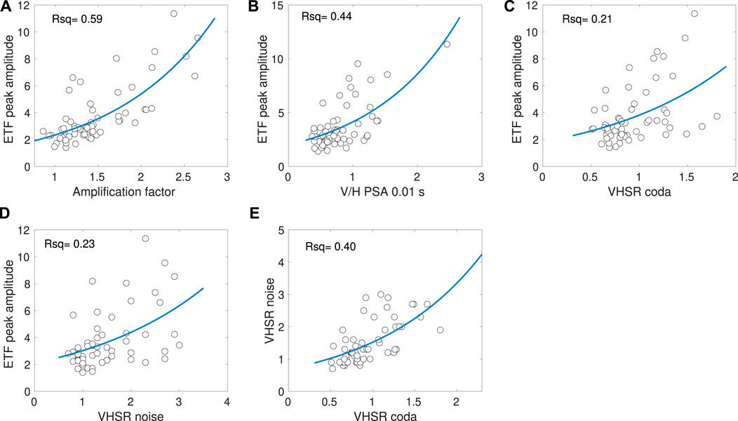
FIGURE 12. Each panel depicts the correlation between the ETF and (A) Amplification factor from maximum amplitudes of earthquake records, (B) the V/H from pseudo-spectral accelerations at 0.01 s, (C) the coda-based peak amplitudes of the VHSR and (D) the noise-based peak amplitudes of the VHSR, and (E) the correlation between the VHSR coda and noise. Each blue line illustrates the fitting function between the two parameters.

Figures 12B–E illustrate the correlation between maximum amplification (ETF peak amplitudes) and three possible single-station proxies for amplification: peak amplitudes from V/H pseudo-spectral accelerations for a period of 0.01 s, coda-based VHSR and noise-based VHSR. These data points are fitted, using A₀ = a*e^b*^P as a functional form, where A₀ represents the peak amplitude and P the input proxy. a and b are the two unknown parameters that are found through the fitting exercise. The correlation coefficient (Rsq) is calculated to qualify the fit. The spatial distributions of peak amplitudes for respectively the ETF (Figure 7) and VHSR (Figures 9G,H) display a similar pattern, but discrepancy still remains between the absolute amplitudes. This is expressed in the relatively low Rsq-values in Figures 12B–D. Still each of the three presented methods makes it possible to identify the borehole sites with potentially high vertical ground motion amplification during an earthquake.

For this study we use mainly local earthquake signals to estimate seismic site-effect in the vertical direction, following for example, Perron et al. (2018); Bommer et al. (2011). These approaches have the disadvantage that they require the occurrence of earthquakes in the first place. For that reason, a comparison between the VHSR of the earthquake signal and from the ambient noise field is made. The noise VHSR reasonably resembles the earthquake VHSR in terms of curve characteristics and peak amplitudes (Figure 12D), hence the noise VHSR can act as first proxy for increased P-wave amplification at certain locations, in case of absence of earthquakes. In general, measurements of noise microtremors have proven to be very informative for site-response estimation and remain a valuable input for seismic site-response zonation (Bonnefoy-Claudet et al., 2006; Molnar et al., 2018). However, the VHSR coda and noise absolute amplitudes have some discrepancies, mainly because the noise is composed of a mixture of surface and body waves. Further discussion about this discrepancy is beyond the scope of this paper.

The 2D full waveform simulations (Figure 5) show that the angle of incidence of the wavefront at the surface near the earthquake epicentre is relatively small $(<20°)$. For the expected range of angles of incidence, the TTFs appear to be quite similar and amplification not influenced by inclining earthquake waves. This also holds for the TTFs of two comparable but different synthetic V_p profiles, showing that the TTFs are not very sensitive to uncertainties in V_p in gas containing shallow subsurface layers, such as peat. Also, the simulations indicate that P-to-S conversion in the shallow subsurface is minor.

The wide range of V/H and ETF peak amplitude distributions found in the Groningen borehole network are consistent with the observations from Ambraseys and Simpson (1996); Bozorgnia et al. (2000); Liu and Tsai (2018); Elgamal and He (2004); Yang and Sato (2000). Empirically we show that vertical ground motion amplification is very site dependent and comprises a different spatial pattern than it is horizontal counterpart. We show that peat content plays an important role in P-wave ground motion amplification. while S-wave amplification is largely controlled by the stiffness of the Holocene sediments (van Ginkel et al., 2019, 2021). These insights are relevant for the Groningen region and as a consequence, it is not recommended to use the standard practise for assigning a single-value fraction of horizontal ground motion in order to assess motion in the vertical direction as suggested by CEN. (2004); Newmark et al. (1973); Loads (2017) is not recommended.

Furthermore, we show that in absence of a borehole network, the methods using a single surface seismometers are a reliable first proxy to highlight locations with likely elevated amplification in the vertical direction. The borehole earthquake transfer functions indicate that mainly the eastern part of Groningen (borehole locations G19, G62, G60, G31, and G37) is experiencing vertical ground motion amplification (Figure 10). These borehole sites are in the vicinity of large industrial facilities and pipeline infrastructure nearby the city of Delfzijl. If high vertical amplifications are persistent at large magnitudes, appreciable levels of vertical loading may be expected.

8 Conclusions

An interdisciplinary approach based on detailed geological and geophysical analyses is performed to asses the potential for local P-wave amplification in an unconsolidated shallow sediment setting. Near-surface P-wave amplification is in the Groningen setting primarily recorded on the vertical component of the borehole seismometers. This study demonstrated empirically and analytically that vertical ground motion amplification occurs especially at sites with low P-wave velocities. Regarding the influence of shallow local geology, it could be shown that peat-generated gas impacts the P-wave velocities. The data richness in Groningen allowed the analysis of borehole earthquake amplification factors and transfer functions as well as a comparison with the analysis of single-station techniques, using local earthquake records and noise data. Qualitatively, there is a good agreement between the earthquake ground motion amplification, as determined with the various approaches. To this extent we showed that surface seismometer recordings can be used as first proxy to indicate the site-effect of ground motion amplification by P-waves to an earthquake. Furthermore, the theoretical transfer functions appear to be quite similar for various angles of incidence, hence the level of amplification is not influenced by inclining earthquake waves.

The P-wave amplifications (up to a factor of 2.7) observed especially at the eastern part of the Groningen study area, illustrate the significance of a detailed study of amplification in the vertical direction. Given that this amplitude distribution shows a different pattern than for the amplification of the horizontal ground motion, we conclude that vertical ground motion amplification by low magnitude earthquakes at shallow depth cannot be treated as an average percentage of horizontal ground motion. In Groningen, unconsolidated sediments with low V_p lead to significant P-wave amplification, and should be considered to be included in predictive ground motion equations. P-to-S wave conversion in the shallow subsurface is found to be unimportant.

Although the gas production in Groningen will be ceased in the coming years, knowledge on vertical ground motion amplification by shallow and low magnitude earthquakes in a soft sedimentary setting is also key in other areas with seismic hazard, either in the Netherlands or at any site across the globe with similar conditions.

Data Availability Statement

Publicly available datasets were analyzed in this study. This data can be found here: http://rdsa.knmi.nl/dataportal/.

Author Contributions

JvG: method development, data analysis, provided input for the 2D simulations, writing of manuscript with input from all co-authors. ER: daily advisor, input on data analysis method and results, performed text input. RW: performed the 2D wave propagation simulations and performed text input. RH: promotor, initiator of this research project, advisor, final text editor.

Funding

This work is funded by EPI Kenniscentrum.

Conflict of Interest

The authors declare that the research was conducted in the absence of any commercial or financial relationships that could be construed as a potential conflict of interest.

Publisher’s Note

All claims expressed in this article are solely those of the authors and do not necessarily represent those of their affiliated organizations, or those of the publisher, the editors, and the reviewers. Any product that may be evaluated in this article, or claim that may be made by its manufacturer, is not guaranteed or endorsed by the publisher.

Acknowledgments

Figures are produced in Matlab, except Figure 1 is produced in QGIS. The authors like to thank Jan Stafleu from TNO for compiling the cumulative thickness maps based on GeoTOP. The authors like to thank the reviewers Mikhail Rodkin and Hamid Zafarani for their valuable input.

Supplementary Material

The Supplementary Material for this article can be found online at: https://www.frontiersin.org/articles/10.3389/feart.2022.812658/full#supplementary-material

References

Ambraseys, N. N., and Simpson, K. A. (1996). Prediction of Vertical Response Spectra in Europe. Earthquake Engng. Struct. Dyn. 25, 401–412. doi:10.1002/(sici)1096-9845(199604)25:4<401::aid-eqe551>3.0.co;2-b

CrossRef Full Text | Google Scholar

Biot, M. A. (1962). Mechanics of Deformation and Acoustic Propagation in Porous media. J. Appl. Phys. 33, 1482–1498. doi:10.1063/1.1728759

CrossRef Full Text | Google Scholar

Bommer, J., Dost, B., Edwards, B., Kruiver, P., Meijers, P., Rodriguez-Marek, A., et al. (2017a). V4 Ground-Motion Model (GMM) for Response Spectral Accelerations, Peak Ground Velocity, and Significant Durations in the Groningen Field. A report prepared for NAM. Available from: https://www.nam.nl/feiten-en-cijfers/onderzoeksrapporten.html.

Google Scholar

Bommer, J. J., Akkar, S., and Kale, O. (2011). A Model for Vertical-To-Horizontal Response Spectral Ratios for Europe and the Middle East. Bull. Seismological Soc. America 101, 1783–1806. doi:10.1785/0120100285

CrossRef Full Text | Google Scholar

Bommer, J. J., Stafford, P. J., Edwards, B., Dost, B., van Dedem, E., Rodriguez-Marek, A., et al. (2017b). Framework for a Ground-Motion Model for Induced Seismic hazard and Risk Analysis in the Groningen Gas Field, the Netherlands. Earthquake Spectra 33, 481–498. doi:10.1193/082916eqs138m

CrossRef Full Text | Google Scholar

Bonilla, L. F., Steidl, J. H., Lindley, G. T., Tumarkin, A. G., and Archuleta, R. J. (1997). Site Amplification in the San Fernando valley, California: Variability of Site-Effect Estimation Using the S-Wave, Coda, and H/V Methods. Bull. Seismological Soc. America 87, 710–730. doi:10.1785/bssa0870030710

CrossRef Full Text | Google Scholar

Bonnefoy-Claudet, S., Cotton, F., and Bard, P.-Y. (2006). The Nature of Noise Wavefield and its Applications for Site Effects Studies. Earth-Science Rev. 79, 205–227. doi:10.1016/j.earscirev.2006.07.004

CrossRef Full Text | Google Scholar

Bozorgnia, Y., and Campbell, K. W. (2016a). Ground Motion Model for the Vertical-To-Horizontal (V/H) Ratios of PGA, PGV, and Response Spectra. Earthquake Spectra 32, 951–978. doi:10.1193/100614eqs151m

CrossRef Full Text | Google Scholar

Bozorgnia, Y., Campbell, K. W., and Niazi, M. (2000). “Observed Spectral Characteristics of Vertical Ground Motion Recorded during Worldwide Earthquakes from 1957 to 1995,” in Proceedings of the 12th World Conference on Earthquake Engineering (Auckland: New Zealand), 2671.

Google Scholar

Bozorgnia, Y., and Campbell, K. W. (2016b). Vertical Ground Motion Model for PGA, PGV, and Linear Response Spectra Using the NGA-West2 Database. Earthquake Spectra 32, 979–1004. doi:10.1193/072814eqs121m

CrossRef Full Text | Google Scholar

Buijze, L., Van Den Bogert, P. A. J., Wassing, B. B. T., Orlic, B., and Ten Veen, J. (2017). Fault Reactivation Mechanisms and Dynamic Rupture Modelling of Depletion-Induced Seismic Events in a Rotliegend Gas Reservoir. Neth. J. Geosciences 96, s131–s148. doi:10.1017/njg.2017.27

CrossRef Full Text | Google Scholar

Cen, E. (2004). 1 Design of Structures for Earthquake Resistance–Part 1: General Rules Seismic Actions and Rules for Buildings. European Committee for Standardization.

Google Scholar

Chin, B.-H., and Aki, K. (1991). Simultaneous Study of the Source, Path, and Site Effects on strong Ground Motion during the 1989 Loma Prieta Earthquake: a Preliminary Result on Pervasive Nonlinear Site Effects. Bull. Seismological Soc. America 81, 1859–1884.

Google Scholar

[Dataset] Knmi, (1993). Netherlands Seismic and Acoustic Network. De Bilt: Royal Netherlands Meteorological Institute. Other/Seismic Network. 10.21944/e970fd34-23b9-3411-b366-e4f72877d2c5.

Google Scholar

Dost, B., Ruigrok, E., and Spetzler, J. (2017). Development of Seismicity and Probabilistic hazard Assessment for the Groningen Gas Field. Neth. J. Geosciences 96, s235–s245. doi:10.1017/njg.2017.20

CrossRef Full Text | Google Scholar

Dost, B., van Stiphout, A., Kühn, D., Kortekaas, M., Ruigrok, E., and Heimann, S. (2020). Probabilistic Moment Tensor Inversion for Hydrocarbon-Induced Seismicity in the Groningen Gas Field, the Netherlands, Part 2: Application. Washington: Bulletin of the Seismological Society of America.

Google Scholar

Elgamal, A., and He, L. (2004). Vertical Earthquake Ground Motion Records: an Overview. J. Earthquake Eng. 8, 663–697. doi:10.1080/13632460409350505

CrossRef Full Text | Google Scholar

Elnashai, A. S., and Papazoglou, A. J. (1997). Procedure and Spectra for Analysis of Rc Structures Subjected to strong Vertical Earthquake Loads. J. Earthquake Eng. 1, 121–155. doi:10.1080/13632469708962364

CrossRef Full Text | Google Scholar

Fjaer, E., Holt, R. M., Horsrud, P., Raaen, A. M., and Risnes, R. (2008). Petroleum Related Rock Mechanics in Developments in Petroleum Science. 2nd edition 53. Amsterdam: Elsevier.

Google Scholar

Hofman, L. J., Ruigrok, E., Dost, B., and Paulssen, H. (2017). A Shallow Seismic Velocity Model for the Groningen Area in the Netherlands. J. Geophys. Res. Solid Earth 122, 8035–8050. doi:10.1002/2017jb014419

CrossRef Full Text | Google Scholar

Jagt, L., Ruigrok, E., and Paulssen, H. (2017). Relocation of Clustered Earthquakes in the Groningen Gas Field. Neth. J. Geosciences 96, s163–s173. doi:10.1017/njg.2017.12

CrossRef Full Text | Google Scholar

Kallioras, S., Correia, A. A., Graziotti, F., Penna, A., and Magenes, G. (2020). Collapse Shake-Table Testing of a clay-URM Building with Chimneys. Bull. Earthquake Eng. 18, 1009–1048. doi:10.1007/s10518-019-00730-0

CrossRef Full Text | Google Scholar

Kato, K., Aki, K., and Takemura, M. (1995). Site Amplification from Coda Waves: Validation and Application to S-Wave Site Response. Bull. Seismological Soc. America 85, 467–477.

Google Scholar

Konno, K., and Ohmachi, T. (1998). Ground-motion Characteristics Estimated from Spectral Ratio between Horizontal and Vertical Components of Microtremor. Bull. Seismological Soc. America 88, 228–241. doi:10.1785/bssa0880010228

CrossRef Full Text | Google Scholar

Korswagen, P. A., Longo, M., Meulman, E., and Rots, J. G. (2019). Crack Initiation and Propagation in Unreinforced Masonry Specimens Subjected to Repeated In-Plane Loading during Light Damage. Bull. Earthquake Eng. 17, 4651–4687. doi:10.1007/s10518-018-00553-5

CrossRef Full Text | Google Scholar

Koymans, M., Ballesta, J. D., Ruigrok, E., Sleeman, R., Trani, L., and Evers, L. (2021). Performance Assessment of Geophysical Instrumentation through the Automated Analysis of Power Spectral Density Estimates. Earth Space Sci., e2021EA001675. doi:10.1029/2021ea001675

CrossRef Full Text | Google Scholar

Kramer, S. L. (1996). Geotechnical Earthquake Engineering. London, United Kingdom: Pearson Education India.

Google Scholar

Kruiver, P. P., Wiersma, A., Kloosterman, F. H., de Lange, G., Korff, M., Stafleu, J., et al. (2017). Characterisation of the Groningen Subsurface for Seismic hazard and Risk Modelling. Neth. J. Geosciences 96, s215–s233. doi:10.1017/njg.2017.11

CrossRef Full Text | Google Scholar

Lermo, J., and Chávez-García, F. J. (1993). Site Effect Evaluation Using Spectral Ratios with Only One Station. Bull. seismological Soc. America 83, 1574–1594. doi:10.1785/bssa0830051574

CrossRef Full Text | Google Scholar

Liu, H.-W., and Tsai, C.-C. (2018). Site Effect of Vertical Motion-Amplification Behavior Observed from Downhole Arrays. J. GeoEngineering 13, 39–48.

Google Scholar

Loads, M. D. (2017). Associated Criteria for Buildings and Other Structures: Asce/sei 7-16. Reston, VA: American Society of Civil Engineers.

Google Scholar

Mad Said, M. J., Zainorabidin, A., and Madun, A. (2015). “Soil Velocity Profile on Soft Soil Using Seismic Refraction,” in Amm (Trans Tech Publications Ltd) (Applied Mechanics and Materials), 773-774, 1549–1554. doi:10.4028/www.scientific.net/amm.773-774.1549

CrossRef Full Text | Google Scholar

Malomo, D., Pinho, R., and Penna, A. (2019). Applied Element Modelling of the Dynamic Response of a Full-Scale clay brick Masonry Building Specimen with Flexible Diaphragms. Int. J. Architectural Heritage, 1–18. doi:10.1080/15583058.2019.1616004

CrossRef Full Text | Google Scholar

Mayeda, K., Koyanagi, S., and Aki, K. (1991). Site Amplification from S-Wave Coda in the Long Valley Caldera Region, California. Bull. Seismological Soc. America 81, 2194–2213. doi:10.1785/bssa0810062194

CrossRef Full Text | Google Scholar

Meijles, E. (2015). De Ondergrond Van Groningen: Een Geologische Geschiedenis. Assen: NAM.

Google Scholar

Molnar, S., Cassidy, J. F., Castellaro, S., Cornou, C., Crow, H., Hunter, J. A., et al. (2018). Application of Microtremor Horizontal-To-Vertical Spectral Ratio (Mhvsr) Analysis for Site Characterization: State of the Art. Surv. Geophys. 39, 613–631. doi:10.1007/s10712-018-9464-4

CrossRef Full Text | Google Scholar

Nakamura, Y. (1989). A Method for Dynamic Characteristics Estimation of Subsurface Using Microtremor on the Ground Surface. Washington: Railway Technical Research Institute. Quarterly Reports 30.

Google Scholar

Nakamura, Y. (2019). What Is the Nakamura Method? Seismological Res. Lett. 90, 1437–1443. doi:10.1785/0220180376

CrossRef Full Text | Google Scholar

Nakata, N., Snieder, R., Kuroda, S., Ito, S., Aizawa, T., and Kunimi, T. (2013). Monitoring a Building Using Deconvolution Interferometry. I: Earthquake-Data Analysis. Bull. Seismological Soc. America 103, 1662–1678. doi:10.1785/0120120291

CrossRef Full Text | Google Scholar

Newmark, N. M., Blume, J. A., and Kapur, K. K. (1973). in Seismic Design Spectra for Nuclear Power plantsTech. Rep. (Urbana, IL: Consulting Engineering Services).

Google Scholar

Perron, V., Gélis, C., Froment, B., Hollender, F., Bard, P.-Y., Cultrera, G., et al. (2018). Can Broad-Band Earthquake Site Responses Be Predicted by the Ambient Noise Spectral Ratio? Insight from Observations at Two Sedimentary Basins. Geophys. J. Int. 215, 1442–1454. doi:10.1093/gji/ggy355

CrossRef Full Text | Google Scholar

Rodriguez-Marek, A., Kruiver, P. P., Meijers, P., Bommer, J. J., Dost, B., van Elk, J., et al. (2017). A Regional Site-Response Model for the Groningen Gas Field. Bull. Seismological Soc. America 107, 2067–2077.

CrossRef Full Text | Google Scholar

Romijn, R. (2017). Groningen Velocity Model 2017. Tech. rep., NAM). Assen: Nederlands Aardolie Maatschappij.

Google Scholar

Rong, M., Li, H., and Yu, Y. (2019). The Difference between Horizontal-To-Vertical Spectra Ratio and Empirical Transfer Function as Revealed by Vertical Arrays. PloS one 14, e0210852. doi:10.1371/journal.pone.0210852

PubMed Abstract | CrossRef Full Text | Google Scholar

Saadeghvariri, M. A., and Foutch, D. A. (1991). Dynamic Behaviour of R/C Highway Bridges under the Combined Effect of Vertical and Horizontal Earthquake Motions. Earthquake Engng. Struct. Dyn. 20, 535–549. doi:10.1002/eqe.4290200604

CrossRef Full Text | Google Scholar

Sánchez-Sesma, F. J., Rodríguez, M., Iturrarán-Viveros, U., Luzón, F., Campillo, M., Margerin, L., et al. (2011). A Theory for Microtremor H/V Spectral Ratio: Application for a Layered Medium. Geophys. J. Int. 186, 221–225. doi:10.1111/j.1365-246x.2011.05064.x

CrossRef Full Text | Google Scholar

Sarmadi, M. A., Heidari, R., Mirzaei, N., and Siahkoohi, H. R. (2021). The Improvement of the Earthquake and Microseismic Horizontal-To-Vertical Spectral Ratio (Hvsr) in Estimating Site Effects. Acta Geophysica, 1–12. doi:10.1007/s11600-021-00619-0

CrossRef Full Text | Google Scholar

Stafleu, J., Maljers, D., Busschers, F. S., Schokker, J., Gunnink, J. L., and Dambrink, R. M. (2021). Models Created as 3‐D Cellular Voxel Arrays. Appl. Multidimensional Geol. Model. Informing Sustain. Hum. interactions shallow subsurface, 247–271. doi:10.1002/9781119163091.ch11

CrossRef Full Text | Google Scholar

Stafleu, J., Maljers, D., Gunnink, J. L., Menkovic, A., and Busschers, F. S. (2011). 3D Modelling of the Shallow Subsurface of Zeeland, the Netherlands. Neth. J. Geosciences 90, 293–310. doi:10.1017/s0016774600000597

CrossRef Full Text | Google Scholar

Su, F., Anderson, J. G., Brune, J. N., and Zeng, Y. (1996). A Comparison of Direct S-Wave and Coda-Wave Site Amplification Determined from Aftershocks of the Little Skull Mountain Earthquake. Bull. Seismological Soc. America 86, 1006–1018.

Google Scholar

van Ginkel, J., Ruigrok, E., and Herber, R. (2019). Assessing Soil Amplifications in Groningen, the Netherlands. First Break 37, 33–38. doi:10.3997/1365-2397.2019026

CrossRef Full Text | Google Scholar

van Ginkel, J., Ruigrok, E., and Herber, R. (2020). Using Horizontal-To-Vertical Spectral Ratios to Construct Shear-Wave Velocity Profiles. Solid Earth 11, 2015–2030. doi:10.5194/se-11-2015-2020

CrossRef Full Text | Google Scholar

van Ginkel, J., Ruigrok, E., Stafleu, J., and Herber, R. (2021). Development of a Country-wide Seismic Site-Response Zonation Map for the Netherlands. Nat. Hazards Earth Syst. Sci. Discuss., 1–34.

Google Scholar

Wapenaar, K., Slob, E., Snieder, R., and Curtis, A. (2010). Tutorial on Seismic Interferometry: Part 2 - Underlying Theory and New Advances. Geophysics 75, 75A211–75A227. doi:10.1190/1.3463440

CrossRef Full Text | Google Scholar

Wong, T. E., Batjes, D. A., and de Jager, J. (2007). Geology of the Netherlands. Amsterdam: The Publishing House of the Royal Netherlands Academy of Arts and Sciences.

Google Scholar

Yang, J., and Lee, C. M. (2007). Characteristics of Vertical and Horizontal Ground Motions Recorded during the Niigata-Ken Chuetsu, Japan Earthquake of 23 October 2004. Eng. Geology. 94, 50–64. doi:10.1016/j.enggeo.2007.06.003

CrossRef Full Text | Google Scholar

Yang, J., and Sato, T. (2000). Interpretation of Seismic Vertical Amplification Observed at an Array Site. Bull. Seismological Soc. America 90, 275–285. doi:10.1785/0119990068

CrossRef Full Text | Google Scholar

Yang, J., and Yan, X. R. (2009). Factors Affecting Site Response to Multi-Directional Earthquake Loading. Eng. Geology. 107, 77–87. doi:10.1016/j.enggeo.2009.04.002

CrossRef Full Text | Google Scholar

Zhu, C., Cotton, F., and Pilz, M. (2020). Detecting Site Resonant Frequency Using HVSR: Fourier versus Response Spectrum and the First versus the Highest Peak Frequency. Washington: Bulletin of the Seismological Society of America.

Google Scholar

Zimmer, M. A., Prasad, M., Mavko, G., and Nur, A. (2007). Seismic Velocities of Unconsolidated Sands: Part 1 - Pressure Trends from 0.1 to 20 MPa. Geophysics 72, E1–E13. doi:10.1190/1.2399459

CrossRef Full Text | Google Scholar

Zwanenburg, C., Konstadinou, M., Meijers, P., Goudarzy, M., König, D., Dyvik, R., et al. (2020). Assessment of the Dynamic Properties of Holocene Peat. J. Geotech. Geoenviron. Eng. 146, 04020049. doi:10.1061/(asce)gt.1943-5606.0002259

CrossRef Full Text | Google Scholar