NWPP-EDH: Numerical weather prediction products evaporation duct regional prediction model

The evaporation duct is a special atmospheric stratification that can affect the propagation path of electromagnetic waves at sea, thus it is crucial for the ability of the radio communication systems. The traditional theoretical models of the evaporation duct often have limited accuracy. The actual observational data from voyages and stations are insufficient, and the existing data-driven evaporation duct height prediction models can only predict a particular point or route but cannot reproduce the regional distribution of the evaporation duct. To address these issues, we propose NWPP-EDH model in this work. The fitting ability of the NWPP-EDH model was tested. Its accuracy was compared with that of the Babin–Young–Carton model, Musson–Gauthier–Bruth model, and the classical Naval Postgraduate School model; compared to these models, the root mean square error (RMSE) of NWPP-EDH model was reduced by 71.8%, 87%, and 60.9%, respectively. Thus, we find that the model shows a better performance than the existing theoretical models.

1 Introduction

The atmospheric duct is a stratification in the atmospheric boundary layer. Ducts exert considerable influence on the propagation of electromagnetic waves. This is because the refractive index decreases sharply with height in the atmospheric boundary layer. Therefore, the electromagnetic wave will bend down abnormally during propagation, resulting in a smaller curvature radius of the electromagnetic wave compared that of the Earth (Kang et al., 2014). Under appropriate frequency and incidence angle conditions, radio waves will be repeatedly refracted within the atmospheric duct; the duct acts as a conductor and facilitates the propagation of the electromagnetic wave beyond the horizon with low energy attenuation. This limits the electromagnetic wave transmission to only the atmospheric stratification range of the duct. Efficient use of atmospheric ducts can not only improve radio communications between ships at sea but also shield the communication equipment in the air from radio interference. Types of atmospheric ducts are evaporation ducts, surface ducts and suspended ducts. The evaporation duct is a special type of surface ducts created by a sharp humidity reduction with increasing altitude. They form frequently in marine environments, with an average occurrence probability higher than 60% in the global sea area. In the northern part of South China Sea (SCS), the occurrence probability of evaporation duct height (EDH) is between 18.18% and 81.82%, in the southern part of SCS the occurrence probability of EDH is between 68.75 and 100% (Ding and Guan, 2012). Generally, evaporation ducts appear lower than 40 m above the sea surface, and hence, they remarkably affect radio communication efficiency.

The EDH directly reflects the lamination height of the evaporation duct and plays an important role in determining the strength of the duct (Liu and Blanc, 1984). EDH is most commonly obtained using theoretical models, and the values of EDH are calculated based on the known meteorological factors, such as wind speed, air temperature, air pressure, relative humidity and sea surface temperature. In 1971, the Jeske model (Paulus, 1985) was proposed, and this model was improved by Paulus in 1985 by using more accurate data to build the Paulus–Jeske (P-J) model (Jeske, 1971). In the 1980s, Gavrilov and coworkers proposed the RSHMU EDH prediction model (Xie and Tian, 2015100), which was mainly used in the former Soviet Union Republics. In 1992, Musson, Gauthier, and Bruth jointly proposed the MGB (Luc et al., 1992) model based on Monin–Obukhov (M-O) similarity theory. In 1997, the Babin–Young–Carton (BYC) model (Steven et al., 1997), which employs the advanced COARE air–sea flux algorithm (Fairall et al., 2003), was put forward. In 2000, Frederickson and coworkers at the Naval Postgraduate School (NPS) proposed the NPS model (Frederickson et al., 2000). In 2001, Liu et al. put forward the pseudo-refractive index model (Liu and Huang, 2001) by adding the concept of a pseudo-refractive index to the P-J model. In 2002, Dai Fushan et al. replaced the M-O similarity theory with the local similarity theory based on the BYC model and developed the local model (Dai and Li, 2002). In 2015, Ding et al. put forward the universal evaporation duct model (Ding et al., 2015). Although theoretical models provide a convenient prediction method for EDH, they have low accuracy and generalizability.

Zhu et al. tried to combine the traditional evaporation duct theoretical model with machine learning and optimized the P-J model by adopting the support vector regression (SVR) method (Zhu et al., 2018). Compared with the P-J model, the obtained SVR_PJ model provides higher accuracy. By using the data collected in the South China Sea, Zhu et al. built the SCS-MLP (Zhu and Zhu, 2018), a multilayer perceptron (MLP) (Allan, 1999) model for predicting the evaporation duct height in the South China Sea. They then showed that their approach significantly improved the P-J model. Zhao et al. also applied back propagation neural network to predict EDH and achieved good results (Zhao and Li, 2020). They further proposed a pure data-driven gradient boosting decision tree (GBDT) EDH prediction model, namely, PDD_GBR, which greatly improved both the accuracy and regional generalization ability of their original model (Zhao et al., 2019). Extreme gradient boosting (XGBoost) is an improved version of the GBDT algorithm (Chen and Tong, 2016); it was adopted by Zhao in 2020 to build the XGBoost EDH prediction model (Zhao et al., 2020). XGBoost is highly efficient in estimating the EDH. The experimental results also showed that its accuracy was remarkably higher than that of the traditional P-J theoretical model. Furthermore, compared with the SCS-MLP and PDD_GBR models, XGBoost EDH prediction model had much higher accuracy and generalization ability.

Compared with the traditional models, the aforementioned machine-learning-based models have higher accuracy and generalization ability for predicting the EDH. However, they require meteorological and hydrological observational data measured on a certain route or at a station. The models are trained with these data, and hence, they cannot reflect the EDH distribution in a particular sea area because of the lack of spatial correlation. Actual observational data from equipment at points and routes at sea are scarce, and hence, the problems of insufficient samples and insufficient model training arise. The actual observational data from voyages and stations are insufficient, and the existing data-driven evaporation duct height prediction models can only predict a particular point or route but cannot reproduce the regional distribution of the evaporation duct. To address these issues, in this study, we used the Yin–He global spectral model (YHGSM) weather prediction products data set for some areas of the SCS. A numerical weather prediction products (NWPP) EDH regional prediction model based on a deep-learning convolutional neural network (CNN) was constructed. It is the first data-driven evaporation duct height regional prediction model. This model was compared with the traditional BYC (Steven et al., 1997), MGB (Luc et al., 1992), and NPS (Frederickson et al., 2000) models. The experimental results showed that our NWPP-EDH model has a remarkably higher accuracy than the traditional models.

2 Brief introduction of the theoretical evaporation duct height model

2.1 Paulus-Jeske model

Paulus-Jeske Model (P-J Model) is the most widely used theoretical evaporation duct height model. In 1985, Paulus improved the Jeske Model (Paulus, 1985) with better data and proposed the Paulus-Jeske Model (Jeske, 1971). P-J model is a classic and effective evaporation duct model. It was applied to the Integrated Refractive Effects Prediction System (IREPS) for evaluating electromagnetic wave propagation and then applied to Advanced Refractive Effects Prediction Systems (AREPS) which was the upgraded version of IREPS. The input parameters of the model are sea surface temperature, air temperature, relative humidity, and wind speed. The atmospheric pressure is assumed to be 1000 hPa.

P-J model used the potential refractive index N_P to replace the atmospheric refractive index N, the potential water vapor pressure to replace the water vapor pressure. Assuming that the potential refractive index is equal to the refractive index, the calculation formula of the potential refractive index is as follows:

${\mathit{N}}_{\mathit{p}}=\frac{\mathbf{77.6}}{\mathit{\theta }}\left(\mathit{P}+\frac{\mathbf{4810}{\mathit{e}}_{\mathit{p}}}{\mathit{T}}\right)(1)$

where the potential water vapor ${\mathit{e}}_{\mathit{p}}$ is:

${\mathit{e}}_{\mathit{p}}={\mathit{e}}^{\mathbf{1}+\frac{\mathbf{1000}}{\mathit{p}}}(2)$

The critical gradient is defined as in terms of the refractive index gradient, and differentiated from Eq. 1

$\frac{\partial {\mathit{N}}_{\mathit{p}}}{\partial \mathit{z}}=\frac{\partial \mathit{N}}{\partial \mathit{z}}-\frac{\partial \mathit{N}}{\partial \mathit{P}}\times \frac{\partial \mathit{P}}{\partial \mathit{z}}(3)$

Using the standard temperature of 15°C, atmospheric pressure of 1000 hPa, and gravitational acceleration g=9.8 m/s², z means height, the critical refractive index gradient is

$\frac{\partial {\mathit{N}}_{\mathit{p}}}{\partial \mathit{z}}=-\mathbf{0.125}(4)$

It is assumed that the index of refraction is a similar variable, and the following conditions are satisfied.

$\frac{\partial {\mathit{N}}_{\mathit{p}}}{\partial \mathit{z}}=\frac{{\mathit{S}}_{{\mathit{N}}_{\mathit{p}}}\mathit{\phi }}{\mathit{\rho }\mathit{k}{\mathit{u}}_{*}\left(\mathit{z}+{\mathit{z}}_{\mathbf{0}}\right)}(5)$

Where is the vertical flux of the potential refractive index, z is the measurement height above 6 m, z₀ is the dynamic roughness, $\phi$ is the universal function, k is the Kalman constant value of 0.4, u_* is the friction speed.

The universal function $\phi$ is a function of z/L and represents the near surface atmospheric stability,

$\mathit{\phi }=\mathbf{1}+{\mathit{\alpha }}_{\mathbf{1}}\frac{\mathit{z}}{\mathit{L}}(6)$

Eq. 6 is the universal function under stable atmospheric conditions, L represents the Monin-Obukhov similarity length and ${\alpha }_1$ is a constant value of 5.2. The universal function under unstable conditions is expressed as follows:

${\mathit{\phi }}^{\mathbf{4}}-\mathbf{4}{\mathit{\alpha }}_{\mathbf{2}}\frac{\mathit{z}}{\mathit{L}}{\mathit{\phi }}^{\mathbf{3}}=\mathbf{1}(7)$

where the ${\alpha }_2$ is constant value of 4.5.

Paulus summed up the empirical relationship (Paulus, 1985) from a large number of experiments, and the predicted value of the evaporation duct height can be obtained by processing Eq. 9 in combination with these empirical relationships. More details about the P-J model can be found in (Jeske, 1971).

2.2 Babin Young Carton model

The widely used P-J model does not account for similar theoretical extensions at low wind speeds and ignores corrections for seawater salinity. The above two points lead to biased prediction accuracy in some cases. By introducing the TOGA COARE air-sea flux algorithm (Steven et al., 1997), Babin proposed the Babin Young Carton Model (BYC model). The BYC model uses the Bulk equation (Fairall et al., 2003) for more accurate water vapor partial pressure calculations, a correction for salinity, and an extension to the M-O similarity theory for low wind speeds. In theory, it is a more advanced traditional evaporation duct height prediction model than the P-J model. The atmospheric refractive index gradient expression in the BYC model can be written as

$\frac{\partial \mathit{N}}{\partial \mathit{z}}=\mathit{A}+\mathit{B}\frac{\partial \mathit{\theta }}{\partial \mathit{z}}+\mathit{C}\frac{\partial \mathit{q}}{\partial \mathit{z}}(8)$

Where the A, B and C, are the middle term of the formula, more details can be found in (Steven et al., 1997). The Monin- Obukhov similarity theory (Grachev and Fairall, 1997) is used to calculate the $\partial \theta /\partial z$ and $\partial q/\partial z$,

$\frac{\mathbf{\partial }\mathit{\theta }}{\mathit{\partial }\mathit{z}}=\frac{{\mathit{\theta }}_{*}{\mathit{\phi }}_{\mathit{h}}}{\mathit{\kappa }\mathit{z}}(9)$

$\frac{\mathit{\partial }\mathit{q}}{\mathit{\partial }\mathit{z}}=\frac{{\mathit{q}}_{*}{\mathit{\phi }}_{\mathit{q}}}{\mathit{\kappa }\mathit{z}}(10)$

When the refractive index gradient $\partial N/\partial z$ =−0.157, the height of the evaporation duct can be determined based on the above formula, and the evaporation duct height under stable or neutral atmospheric conditions is

${\mathit{z}}_{\mathit{E}\mathit{D}\mathit{H}}=\frac{-\left(\mathit{B}{\mathit{\theta }}_{*}+\mathit{C}{\mathit{q}}_{*}\right)}{\mathit{\kappa }\left(\mathit{A}+\mathbf{0.157}\right)+\frac{\mathbf{5}}{\mathit{L}}\left(\mathit{B}{\mathit{\theta }}_{*}+\mathit{C}{\mathit{q}}_{*}\right)}(11)$

Under unstable atmospheric conditions is

${\mathit{z}}_{\mathit{E}\mathit{D}\mathit{H}}=\frac{-\left(\mathit{B}{\mathit{\theta }}_{*}+\mathit{C}{\mathit{q}}_{*}\right){\mathit{\phi }}_{\mathit{h}}}{\mathit{\kappa }\left(\mathit{A}+\mathbf{0.157}\right)}(12)$

The ${\theta }_{*}$, $q_{*}$ , ${\phi }_h$ and ${\phi }_q$ are the parameters from the COARE air-sea flux algorithm, more details can be found in (Fairall et al., 2003).

Based on the COARE air-sea flux algorithm, the BYC model can describe physical phenomena more closely and is a deeper extension of the Monin-Obukhov similarity theory. From the calculation process of the BYC model we can find that the BYC model has higher complexity and more physical constraints. More empirical parameters are involved in the calculation process, which is prone to large deviations in the inapplicable air-sea environment.

2.3 Musson Gauthier Bruth model

Based on the Monin-Obukhov similarity theory, Musson-Gennon, Gauthier and Bruth proposed the Musson Gauthier Bruth model (MGB model) in 1992 (Luc et al., 1992), which takes the air temperature, air pressure, relative humidity, wind speed and sea surface temperature measured at a certain height near the sea as input parameters. The MGB model uses a parametric approach for calculating near-surface fluxes to calculate the characteristic paramenters of potential temperature and humidity, and establishes atmospheric stability through the empirical relationship between Richardson number and similarity length. This model has two calculation processes: iterative method and analytical method. This paper only briefly introduces the MGB model that adopts the iterative calculation process. The algorithm of the iterative MGB model is similar to the BYC model, both based on the iterative loop of the atmospheric refractive index gradient Eq. 3. Evaporation duct height determined by the iterative algorithm is expressed as follows:

${\mathit{z}}_{\mathit{E}\mathit{D}\mathit{H}}=\frac{{\mathit{S}}_{\mathbf{0}}}{\mathbf{1}-\mathbf{6.4}\left({\mathit{S}}_{\mathbf{0}}/\mathit{L}\right)}\left(\mathit{L}⩾\mathbf{0}\right)(13)$

${\mathit{z}}_{\mathit{E}\mathit{D}\mathit{H}}=\frac{{\mathit{S}}_{\mathbf{0}}}{\mathbf{1}-\mathbf{9}\left({\mathit{h}}_{\mathit{c}}/\mathit{L}\right)}\left(\mathit{L}<\mathbf{0}\right)(14)$

Where $S_0$ is expressed as follows:

${\mathit{S}}_{\mathbf{0}}=\frac{\mathit{B}{\mathit{\theta }}_{*}+\mathit{C}{\mathit{q}}_{*}}{\mathit{\kappa }\left(-\mathbf{0.157}-\mathit{A}\right)}(15)$

The MGB model proposed by the French has been widely used in the seas near Europe, and also has applications in the seas near Asia (Cook, 2016).

2.4 Naval Postgraduate School model

Frederickson of the U.S. Naval Graduate School proposed Naval Postgraduate School model (NPS model) in 2000. The difference from the above theoretical model is that the NPS model calculates the profile of the atmospheric modified refractive index through the profiles of temperature, humidity and air pressure. Then determines the evaporation duct height at the position of the minimum value of the modified refractive index. In the NPS model, the vertical profile of temperature T and specific humidity q in the near-surface layer is expressed as

$\begin{array}{c}\mathit{T}\left(\mathit{z}\right)={\mathit{T}}_{\mathbf{0}}+\frac{{\mathit{\theta }}_{*}}{\mathit{\kappa }}\left[\mathit{ln}\left(\frac{\mathit{z}}{{\mathit{z}}_{\mathbf{0}\mathit{t}}}\right)-{\mathit{\psi }}_{\mathit{h}}\left(\frac{\mathit{z}}{\mathit{L}}\right)\right]-{\mathit{\Gamma }}_{\mathit{d}}\mathit{z}\\ \mathit{q}\left(\mathit{z}\right)={\mathit{q}}_{\mathbf{0}}+\frac{{\mathit{q}}_{*}}{\mathit{\kappa }}\left[\mathit{ln}\left(\frac{\mathit{z}}{{\mathit{z}}_{\mathbf{0}\mathit{t}}}\right)-{\mathit{\psi }}_{\mathit{h}}\left(\frac{\mathit{z}}{\mathit{L}}\right)\right]\end{array}(16)$

where T(z) and q(z) are the air temperature and specific humidity at height z. $T_0$ and $q_0$ are the sea surface temperature and specific humidity. ${\theta }_{*}$ and $q_{*}$ are the characteristic scales of potential temperature $\theta$ and the specific humidity q, $\kappa$ is the Kalman constant, $z_{0t}$ is the temperature roughness height, ${\psi }_h$ is the temperature universal function, ${\Gamma }_d$ is the dry adiabatic lapse rate, and L is the similarity length.

The NPS model adopts the advanced COARE3.0 air-sea flux algorithm (Fairall et al., 2003) and the stability correction function under stable atmospheric conditions (Grachev and Fairall, 1997). The temperature stability correction function is expressed as follows

${\mathit{\psi }}_{\mathit{h}}=-\frac{{\mathit{b}}_{\mathit{h}}}{\mathbf{2}}\mathit{ln}\left(\mathbf{1}+{\mathit{c}}_{\mathit{h}}\mathit{\xi }+{\mathit{\xi }}^{\mathbf{2}}\right)\left(-\frac{{\mathit{a}}_{\mathit{h}}}{{\mathit{B}}_{\mathit{h}}}+\frac{{\mathit{b}}_{\mathit{h}}{\mathit{c}}_{\mathit{h}}}{\mathbf{2}{\mathit{B}}_{\mathit{h}}}\right)\times \left(\mathit{ln}\frac{\mathbf{2}\mathit{\xi }+{\mathit{c}}_{\mathit{h}}{\mathit{B}}_{\mathit{h}}}{\mathbf{2}\mathit{\xi }+{\mathit{c}}_{\mathit{h}}+{\mathit{B}}_{\mathit{h}}}-\mathit{ln}\frac{{\mathit{c}}_{\mathit{h}}-{\mathit{B}}_{\mathit{h}}}{{\mathit{c}}_{\mathit{h}}+{\mathit{B}}_{\mathit{h}}}\right)(17)$

where $\xi$ = z/L, $a_h$ =$b_h$ =5, $c_h$ =3, $B_h$ =$\sqrt{5}$.

The NPS model obtains the pressure profile by integrating the hydrostatic equations and the ideal gas law simultaneously, as shown in the following equation

$\mathit{p}\left({\mathit{z}}_{\mathbf{2}}\right)=\mathit{p}\left({\mathit{z}}_{\mathbf{1}}\right)\mathit{exp}\left(\frac{\mathit{g}\left({\mathit{z}}_{\mathbf{1}}-{\mathit{z}}_{\mathbf{2}}\right)}{\mathit{R}\overline{{\mathit{T}}_{\mathit{v}}}}\right)(18)$

where $p\left(z_1\right)$, $p\left(z_2\right)$ are the air pressure measured at the heights $z_1$ and $z_2$, R is the dry air gas constant, g is the gravitational acceleration, $\overline{T_v}$ is the average value of the virtual potential temperature at the heights $z_1$ and $z_2$.

The water vapor pressure profile is expressed as follows:

$\mathit{e}=\frac{\mathit{q}\mathit{p}}{\mathit{\epsilon }+\left(\mathbf{1}-\mathit{\epsilon }\right)\mathit{q}}(19)$

where the $\epsilon$ is the constant value of 0.622.

The atmospheric refractive index profile can be calculated from the temperature, pressure, and water vapor pressure profile obtained by the above formula, so as to further determine the evaporation duct height. The NPS model combines advanced air-sea flux algorithms, it is an advanced theoretical model of evaporation duct height, which has good prediction performance in many sea areas (Yang et al., 2016).

3 Evaporation duct regional prediction model bases on convolutional neural network

The convolutional neural network is a type of neural network that is specially used to process data with similar grid structures. Because the convolution operation is used instead of some common matrix multiplications, a convolutional neural network has a good performance in information extraction form grid data. Convolutional neural networks can reduce the data dimensions while retaining the original information in the data and can transform high-dimensional, large-scale data into low-dimensional, small-scale data to improve data-processing efficiency (Long and Shelhamer, 2015). In this study, the NWPP data were used, and the data type was a two-dimensional (2D) grid, more details about the data please read Section 3.1. Hence, a convolutional neural network was selected to construct the regional prediction model of EDH. Combined with the specific practical application requirements, the U-net was used as the reference network to construct the regional prediction model based on the convolutional network.

3.1 Data set

The data set of this experiment was derived from the YHGSM. NWPP data from a region of the SCS from 16 November 2020 to 20 November 2020.

The YHGSM (Yang et al., 2015; Yin et al., 2018; Peng et al., 2020; Yin et al., 2021) is a numerical weather forecast model developed by the National University of Defense and Technology. Its products data have a relatively stable system error, and the data are provided in a data set for machine learning research in meteorology.

The data are a constant longitude-and-latitude grid data with wind speed, air temperature, atmospheric pressure, relative humidity, and SST at a height of 10 m. Figure 1 shows the location of the test area.

FIGURE 1

FIGURE 1. Structure of the numerical weather prediction products (NWPP) model.

On the premise that the above meteorological elements of each point are known, the label value of EDH is calculated following the method given in reference (Patterson and Hattan, 1994). Due to the space limitations, please find more details in the reference. The calculation steps are as follows:

•Step 1: Judge whether the wind speed is less than 0.005144 m/s. If yes, EDH is recorded as 0, if not, continue.

•Step 2: Calculate the bulk Richardson number.

•Step 3: Calculate the M-O length using the bulk Richardson number and empirical formula.

•Step 4: According to the air–sea stability conditions, calculate the EDH by selecting the suitable calculation formula.

Due to the space limitations, please refer to the reference (Jeske, 1971) and reference (Patterson and Hattan, 1994) to get more details.

The EDH calculated by the aforementioned method is used as the label value, and it is related to the corresponding meteorological elements such as temperature, air pressure, relative humidity, wind speed, and SST.

Our data set has a 40 × 48 grid, where each grid point had 72-h forecast data for 5 days. For each day, forecasts were made twice, at 00:00 and at 12:00. Therefore, our 5-day data set has 2 × 5 × 40 × 48 × 73 = 1401600 data samples.

3.2 U-net

The U-net is a network based on a fully connected convolutional neural network (Ronneberger and Fischer, 2015). It was initially designed for medical image segmentation. The U-net has an inbuilt ingenious data enhancement scheme that is realized by dividing a single large image into subgraphs, thereby directly solving the problem of insufficient training sample size. The construction model based on the U-net can solve the problem of a minor data grid. The U-net structure also has an optimized training process. It also adopts a new feature fusion method based on splicing to ensure that the features transmitted in the U-shaped network structure do not suffer any loss of the edge features and that the learning of in-depth and shallow features are considered. These features enable the U-net to learn the sample data features comprehensively and efficiently. The NWPP grid data used in this study needs a deep-learning network to cover the data characteristics. Based on the U-net network structure, a deep-learning model can be constructed.

3.3 The construction of evaporation duct regional model based on convolutional neural network

3.3.1 The basic structure of the neural network

The traditional theoretical model of EDH describes the nonlinear relationship between the input vector and the EDH. The mathematical relationship is shown as follows

$\mathit{E}\mathit{D}\mathit{H}=\mathit{f}\left(\mathit{S}\mathit{S}\mathit{T},{\mathit{T}}_{\mathit{a}},\mathit{R}\mathit{H},\mathit{U},\mathit{P}\right)(20)$

It is a function of the input meteorological and hydrological elements. The input elements are the sea surface temperature (SST), air temperature ($T_{\mathrm{a}}$), relative humidity ($RH$), wind speed ($U$), and pressure ($P$). EDH is the function value.

The traditional theoretical models are semiempirical physical models based on the M-O similarity theory. The traditional models describe the complex physical relationship between the fundamental meteorological factors and EDH.

The practical problem to be solved in this study is to realize the regional distribution prediction function of EDH in a specific sea area. Hence, we decided to construct the convolutional neural network deep-learning model combined with the two-dimensional grid NWPP data type. The U-net structure is a neural network structure suitable for the two-dimensional grid NWPP data type. Therefore, the U-net structure will be used as the basic framework of the model, and the regional prediction model of EDH based on a convolutional neural network is constructed through modification and adjustment.

We used the U-net structure as the basic framework because our data were 40 × 48 two-dimensional grid data, and we chose two-level data sampling to achieve good training results. The basic framework of our model is a seven-layer neural network structure with three modules, for the encoding, decoding, and bridge functions. Table 1 lists the parameters of the NWPP-EDH model.

TABLE 1

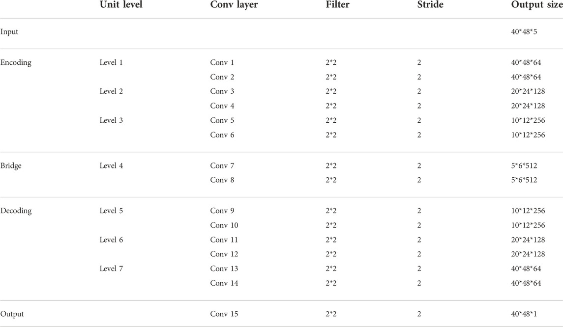
TABLE 1. Numerical weather prediction products (NWPP) model parameters.

The input data matrix was transformed into feature coding in the coding module. The decoding module was used to recover the feature coding into the regression problem of each element in the matrix. The bridge module was used to connect the coding and decoding function modules. Each convolution module contained a batch normalization layer to alleviate overfitting. The rectified linear activation (ReLU) function was selected as the activation layer. The specific structure of the model is shown in Figure 2.

FIGURE 2

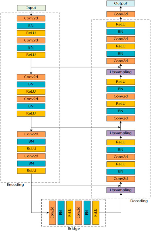
FIGURE 2. Test area location in the South China Sea (SCS).

3.3.2 Loss function

After obtaining the two-dimensional numerical prediction grid data of a particular area and determining the structure of the neural network, we aimed to adjust the network parameters to enable the network to obtain more accurate EDH prediction results. To obtain accurate prediction results, the difference between the predicted value of the model output and the actual value should be minimized. We used the mean square error as the loss function.

The loss function of the model is calculated as follows:

$\mathit{M}\mathit{S}\mathit{E}=\frac{\mathbf{1}}{\mathit{n}}{\displaystyle \sum }_{\mathit{i}=\mathbf{1}}^{\mathit{n}}{\left(\mathit{y}\_\mathit{p}\mathit{r}\mathit{e}\mathit{d}-\mathit{y}\_\mathit{r}\mathit{e}\mathit{a}\mathit{l}\right)}^{\mathbf{2}}(21)$

In the above formula, y is obtained from the output value, and the label value of the y_pred is the output value of the model, and y_real is the true value of EDH.

4 Experiments and the results analysis

To evaluate the performance of the NWPP-EDH model, we used the BYC, MGB, and NPS models as the benchmark models for comparative experiments. We used 80% of the total data as the training set and the remaining 20% of the data as the test set to evaluate the NWPP-EDH model.

Figure 3 shows the regional distribution prediction of the EDH in the selected test area by NWPP-EDH model. The axis scales of the figure represent the longitude and latitude. The EDH distribution in this area was mainly in the range of 10–20 m. Under the influence of special natural conditions, the EDH was zero in some areas; in other words, there was no evaporation duct in these areas.

FIGURE 3

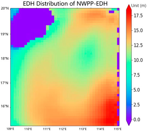
FIGURE 3. Evaporation duct height (EDH) distribution prediction of the NWPP-EDH model.

Square of Correlation Coefficient (SCC) was used as an index to evaluate the goodness of fit of the prediction results and true values. It is a value in the (0,1) interval, and closer the value is to 1, the better is the goodness of fit. The higher the degree of interpretation of independent variables to dependent variables, the stronger is the ability of the model to fit the changing trend of the real values. The SCC is calculated as follows

$\mathit{S}\mathit{C}\mathit{C}=\frac{{\left(\mathit{n}{\displaystyle \sum }_{\mathit{i}=\mathbf{1}}^{\mathit{n}}\mathit{f}\left({\mathit{x}}_{\mathit{i}}\right){\mathit{y}}_{\mathit{i}}-{\displaystyle \sum }_{\mathit{i}=\mathbf{1}}^{\mathit{n}}\mathit{f}\left({\mathit{x}}_{\mathit{i}}\right){\mathit{y}}_{\mathit{i}}{\displaystyle \sum }_{\mathit{i}=\mathbf{1}}^{\mathit{n}}{\mathit{y}}_{\mathit{i}}\right)}^{\mathbf{2}}}{\left(\mathit{n}{\sum }_{\mathit{i}=\mathbf{1}}^{\mathit{n}}{\mathit{f}\left({\mathit{x}}_{\mathit{i}}\right)}^{\mathbf{2}}-{\left({\displaystyle \sum }_{\mathit{i}=\mathbf{1}}^{\mathit{n}}\mathit{f}\left({\mathit{x}}_{\mathit{i}}\right)\right)}^{\mathbf{2}}\right)\left(\mathit{n}{\displaystyle \sum }_{\mathit{i}=\mathbf{1}}^{\mathit{n}}{{\mathit{y}}_{\mathit{i}}}^{\mathbf{2}}-{\left({\displaystyle \sum }_{\mathit{i}=\mathbf{1}}^{\mathit{n}}{\mathit{y}}_{\mathit{i}}\right)}^{\mathbf{2}}\right)}(22)$

To improve the generalization ability of the training model, the model scrambled the data in the training and prediction processes. Hence, the effect of the fitting curve will not be the same every time. To verify the fitting ability of the model more reasonably, we conducted three experiments and took the average SCC value, as shown in Table 2.

TABLE 2

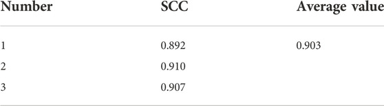
TABLE 2. SCC of the NWPP-EDH model.

The average SCC value of the NWPP-EDH model was 0.903 in three experiments. This value proves that the NWPP-EDH model has an excellent ability to fit the actual values. Thus, the model is proved to be reasonable.

The root means square error (RMSE) was used to evaluate the accuracy of the model. The RMSE reflects the accuracy of the model in predicting the height of the evaporation duct. The lower the RMSE value, the better is the prediction accuracy. The RMSE is calculated as follows.

$\mathit{R}\mathit{M}\mathit{S}\mathit{E}=\sqrt{\frac{1}{n}{{\displaystyle \sum }_{i=1}^n\left(\mathit{f}\left({\mathit{x}}_{\mathit{i}}\right)-{\mathit{y}}_{\mathit{i}}\right)}^2}(23)$

As mentioned earlier, 80% of the data set was used as the training set, and the remaining 20% was used as the test set. Based on the prediction results of the NWPP, BYC, MGB, and NPS models on each grid point and the label value of the corresponding grid point, the RMSE values of the four models were calculated based on the test set (see Table 3).

TABLE 3

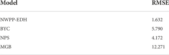
TABLE 3. RMSE indices of the NWPP-EDH, Babin-young-carton (BYC), naval postgraduate school (NPS), and musson gauthier Bruth (MGB) model.

The RMSE of the NWPP-EDH model is much smaller than that of the BYC, MGB, and NPS models. The RMSE of the NWPP-EDH model is less than that of the RMSE of the NWPP model is 71.8%, 87%, and 60.9% lower than that of the BYC, MGB, and NPS models, respectively.

In particular, the MGB model has a substantial error in the target sea area, while the NPS and BYC models have relatively normal prediction effects. This is because MGB is widely used in Europe, and the empirical parameters of the model mainly come from the actual observations in the European sea area. Compared with the BYC and NPS models that are combined with the advanced COARE air–sea algorithm, the MGB model has much poorer generalization ability and ability to describe actual physical phenomena.

Figure 4 shows the error distributions of the NWPP, MGB, BYC, and NPS models, showing the error distribution of each model in a 40 × 48 data grid. The specific calculation method is to average the absolute value of the difference between the predicted and actual values of each element in each 40 × 48 matrix in the test set. The error distribution map reflects the accuracy of the model prediction value. In Figure 4, the deeper the blue, the less is the error of the model. Almost all of the picture for the NWPP-EDH model is dark blue, indicating that the NWPP-EDH model has a small prediction error. The model with the second-best performance is the NPS model, for which most of the map is in blue with a little green. However, the NPS model has significant errors at some grid points, and the effect of this model is not stable. The effect of the BYC model is relatively uniform, and a considerable portion with green in the error distribution diagram indicates that the model has specific errors. The MGB model has remarkable errors in the sea area, and there are large areas covered in yellow and green in the error distribution map, indicating the poor regional prediction effect of this model.

FIGURE 4

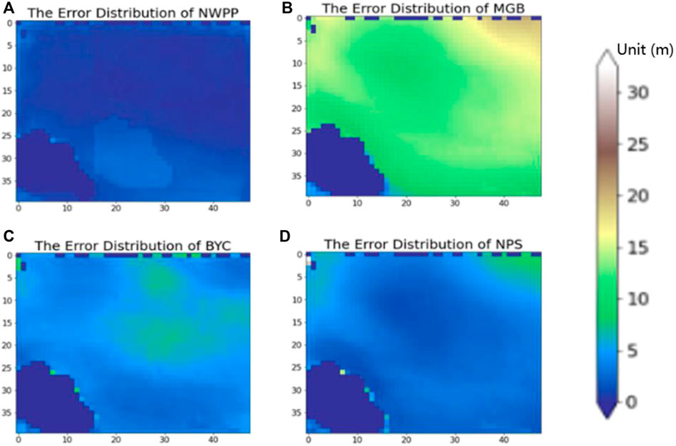
FIGURE 4. Error distributions of the four models: (A) the NWPP-EDH model, (B) is the MGB model, (C) the BYC model, and (D) the NPS model.

5 Conclusion

The traditional evaporation duct theoretical models have limited accuracy, the actual observation data of voyages and stations are not enough and the existing data-driven evaporation duct height prediction models cannot prediction regional distribution of the evaporation duct. To address these issues, in this paper, we propose the NWPP-EDH model. Compared with the traditional models of BYC, MGB, and NPS, the NWPP-EDH model has 71.8%, 87%, and 60.9% decline rates, respectively, in RMSE, which shows that the NWPP-EDH model has outstanding performance in the regional prediction of evaporation duct height. More grid data will be used to propose a more universal and more extensive evaporation duct height regional prediction model in future research (Steven and Dockery, 2002).

Data availability statement

The datasets presented in this article are not readily available because the data for the study is derived from the YHGSM. The YHGSM is the belonging of the National University of Defense Technology from China. Requests to access other datasets should be directed to the author, chaixingyu1997@nudt.edu.cn.

Author contributions

Conceptualization, JL and XC; methodology, XC; software, XC; validation, XC and YH; formal analysis, XC and JL; investigation, XC; resources, XC and JL; data curation, JZ; writing—original draft preparation, XC; writing—review and editing, JL and JZ; visualization, XC; supervision, JL and JZ; project administration, XC; funding acquisition, JZ and XZ.

Funding

This research was funded by National Natural Science Foundation of China (XZ, grant number 41775027).

Acknowledgments

We thank all the editors and reviewers for their comments that significantly improved the presentation of this article. We thank all the partners in the laboratory for their spiritual support.

Conflict of interest

The authors declare that the research was conducted in the absence of any commercial or financial relationships that could be construed as a potential conflict of interest.

Publisher’s note

All claims expressed in this article are solely those of the authors and do not necessarily represent those of their affiliated organizations, or those of the publisher, the editors and the reviewers. Any product that may be evaluated in this article, or claim that may be made by its manufacturer, is not guaranteed or endorsed by the publisher.

References

Allan, P. (1999). Approximation theory of the MLP model in neural networks. Acta Numer. 8, 143–195. doi:10.1017/s0962492900002919

CrossRef Full Text | Google Scholar

Chen, T., and Tong, H. (2016). XGBoost: Extreme gradient boosting.XGBoost, USA

Google Scholar

Cook, J. (2016). A sensitivity study of weather data inaccuracies on evaporation duct height algorithms. Radio Sci. 26, 731–746. doi:10.1029/91rs00835

CrossRef Full Text | Google Scholar

Dai, F., and Li, Q. (2002). Atmospheric Duct and its military applications. Beijing, China: People’s Liberation Army Publishing House.

Google Scholar

Ding, J., Fei, J., Huang, X., Cheng, X., Hu, X., and Ji, L. (2015). Development and validation of an evaporation duct model. Part i: Model establishment and sensitivity experiments. J. Meteorol. Res. 29, 467–481. doi:10.1007/s13351-015-3238-4

CrossRef Full Text | Google Scholar

Ding, X., and Guan, Z. (2012). Characteristics of evaporation duct over the south China sea during 1998 summer monsoon. J. Trop. Meteorology 28, 905–910.

Google Scholar

Fairall, C., Bradley, E., Hare, J. E., Grachev, A. A., and Edson, J. B. (2003). Bulk parameterization of air-sea fluxes: Updates and verification for the COARE algorithm. J. Clim. 16, 571–591. doi:10.1175/1520-0442(2003)016<0571:bpoasf>2.0.co;2

CrossRef Full Text | Google Scholar

Frederickson, P. A., Davidson, K. L., Zeisse, C. R., and Bendall, C. S. (2000). Estimating the refractive index structure parameter (C₂) over the ocean using bulk methods. J. Appl. Meteorology 39, 1770–1783. doi:10.1175/1520-0450-39.10.1770

CrossRef Full Text | Google Scholar

Grachev, A., and Fairall, C. (1997). Dependence of the Monin-Obukhov stability parameter on the bulk Richardson number over the ocean. J. Appl. Meteor. 36, 406–414. doi:10.1175/1520-0450(1997)036<0406:dotmos>2.0.co;2

CrossRef Full Text | Google Scholar

Jeske, H. (1971). The state of radar range prediction over sea in tropospheric radio wave propagation, part II. AGARD CP 70.

Google Scholar

Kang, S., Zhang, Y., and Wang, Z. (2014). Atmospheric duct in troposphere environment. Beijing, China: Science Press.

Google Scholar

Liu, C. G., and Huang, J. Y. (2001). Modeling evaporation duct over sea with pseudo-refractivity and similarity theory. Acta Electron. Sin. 29, 970–972.

Google Scholar

Liu, W., and Blanc, T. (1984). The Liu, Katsaros, and Businger (1979) bulk atmospheric flux computational iteration program in FOR-TRAN and BASIC. Washington, D C, USA: Naval Research Laboratory.

Google Scholar

Long, J., and Shelhamer, E. (2015). Fully convolutional networks for semantic segmentation. Proceedings of the . CVPR, Apr., Boston, MA, USA 3431–3440.

CrossRef Full Text | Google Scholar

Luc, M., Sylvie, G., and Eric, B. (1992). A simple method to determine evaporation duct height in the sea surface boundary layer. Radio Sci. 27, 635–644. doi:10.1029/92rs00926

CrossRef Full Text | Google Scholar

Patterson, W., and Hattan, C. P. (1994). Engineer’s refractive effects prediction system (EREPS); naval command. San Diego, CA, USA: Control and Ocean Surveillance Center.

Google Scholar

Paulus, R. (1985). Practical application of an evaporation duct model. Radio Sci. 20, 887–896. doi:10.1029/rs020i004p00887

CrossRef Full Text | Google Scholar

Peng, J., Zhao, J., Zhang, W., Zhang, L., Wu, J., and Yang, X. (2020). Towards a dry-mass conserving hydrostatic global spectral dynamical core in a general moist atmosphere. Q. J. R. Meteorol. Soc. 146 (732), 3206–3224. doi:10.1002/qj.3842

CrossRef Full Text | Google Scholar

Ronneberger, O., and Fischer, P. (2015). U-Net: Convolutional networks for biomedical image segmentation. Proceedings of the MICCAI. Munich, Germany, 234–241.

CrossRef Full Text | Google Scholar

Steven, M., and Dockery, G. D. (2002). LKB-based evaporation duct model comparison with buoy data. J. Appl. Meteor. 41, 434–446. doi:10.1175/1520-0450(2002)041<0434:lbedmc>2.0.co;2

CrossRef Full Text | Google Scholar

Steven, M., George, S., and James, A. C. (1997). A new model of the oceanic evaporation duct. J. Appl. Meteor. 36, 193–204. doi:10.1175/1520-0450(1997)036<0193:anmoto>2.0.co;2

CrossRef Full Text | Google Scholar

Xie, L., and Tian, B. (2015). Study on evaporation duct RSHMU model in tropical waters. Ship Electron. Eng. 35, 88–90.

Google Scholar

Yang, J., Song, J., Wu, J., Ren, K., and Leng, H. (2015). A high-order vertical discretization method for a semi-implicit mass-based non-hydrostatic kernel. Q. J. R. Meteorol. Soc. 141, 2880–2885. doi:10.1002/qj.2573

CrossRef Full Text | Google Scholar

Yang, S., Li, X., and Wu, J. (2016). Adaptability research of evaporation duct predication model based on NPS model. J. Electron. Meas. Instrum. 30, 1899–1906.

Google Scholar

Yin, F., Song, J., Wu, J., and Zhang, W. (2021). An implementation of single-precision fast spherical harmonic transform in Yin–He global spectral model. Q. J. R. Meteorol. Soc. 147, 2323–2334. doi:10.1002/qj.4026

CrossRef Full Text | Google Scholar

Yin, F., Wu, G., Wu, J., Zhao, J., and Song, J. (2018). Performance evaluation of the fast spherical harmonic transform algorithm in the Yin–He global spectral model. Mon. Weather Rev. 146, 3163–3182. doi:10.1175/mwr-d-18-0151.1

CrossRef Full Text | Google Scholar

Zhao, W., and Li, J. (2020).Research on evaporation duct height prediction based on back propagation neural network, IET Microwaves, Antennas Propag., 14. 1547–1554. Institution of Engineering & Technology).

CrossRef Full Text | Google Scholar

Zhao, W., Li, J., Zhao, J., Zhao, D., Lu, J., and Wang, X. (2020). XGB model: Research on evaporation duct height prediction based on XGBoost algorithm. Radioengineering 29, 81–93. doi:10.13164/re.2020.0081

CrossRef Full Text | Google Scholar

Zhao, W., Li, J., Zhao, J., Zhao, D., and Zhu, X. (2019). PDD_GBR: Research on evaporation duct height prediction based on gradient boosting regression algorithm. Radio Sci. 54, 949–962. doi:10.1029/2019rs006882

CrossRef Full Text | Google Scholar

Zhu, X., Li, J., Zhu, M., Jiang, Z., and Li, Y. (2018). An evaporation duct height prediction method based on deep learning. IEEE Geosci. Remote Sens. Lett. 15, 1307–1311. doi:10.1109/lgrs.2018.2842235

CrossRef Full Text | Google Scholar

Zhu, X., and Zhu, M. (2018). An optimization research of evaporation duct prediction models based on a deep learning method, Proceedings of the 2018 2nd IEEE advanced information management, communicates, electronic and automation control conference. Xi’an, China.

CrossRef Full Text | Google Scholar