Induced microearthquakes predict permeability creation in the brittle crust

Predicting the evolution of permeability accurately during stimulation at the reservoir scale and at the resolution of individual fractures is essential to characterize the fluid transport and the reactive/heat-transfer characteristics of reservoirs where stress exerts significant control. Here, we develop a hybrid machine learning (ML) model to visualize in situ permeability evolution for an intermediate-scale (∼10 m) hydraulic stimulation experiment. This model includes an ML model that was trained using the well history of flow rate and wellhead pressure and MEQ data from the first three stimulation episodes to predict average permeability from the statistical features of the MEQs alone for later episodes. Moreover, a physics-inspired model is integrated to estimate in situ fracture permeability spatially. This method relates fracture permeability to fracture dilation and scales dilation to the equivalent MEQ magnitude, according to laboratory observations. The seismic data are then applied to define incremental changes in permeability in both space and time. Our results confirm the excellent agreement between the ground truth and model-predicted permeability evolution. The resulting permeability map defines and quantifies flow paths in the reservoir with the averaged permeability comparing favorably with the ground truth of permeability.

Introduction

Enhanced geothermal systems (EGSs) could provide plentiful and continuous carbon-free energy for the increasing global demand of electric power (Williams et al., 2008; Kneafsey et al., 2018; Kneafsey et al., 2019) and have significant potential to shift the current dependence on fossil fuels (Fridleifsson, 2018). The amount of geothermal energy that can be economically extracted depends on reservoir temperature, utilizable reservoir volume (Bauer et al., 2019), and rates of fluid mass and heat transfer, which are in turn controlled by petrophysical parameters (Laubach et al., 2009; Bauer et al., 2017; Kushnir et al., 2018). The ability to create a reservoir and to predict permeability evolution before, during, and after stimulation at the reservoir scale and at the resolution of individual fractures is essential to accurately estimate fluid mass transfer and heat recovery from the reservoir.

The difficulty in predicting permeability evolution using purely numerical physics-based geomechanical models is that the description of the state of the system to its consequent behavior is often very complicated. This comes from the nonlinear nature of the variables that define the system underlying the time-evolution. For example, the permeability of new fractures is highly stress dependent. The evolution of the fracture permeability can be evaluated from fracture compaction/dilation or propagation—provided the geometric evolution and connectivity is known/predictable. However, the complexity of this nonlinear response and reinforcing feedback linking changes in the reservoir pressure to changes in permeability renders such problems intrinsically ill-constrained and ill-defined. This situation is compounded by the reality that initial conditions are also poorly constrained and perhaps unknowable. Additionally, these models rely on the integration of multiple geologic, geochemical, and geophysical input data that are usually collected during and after well stimulation. This innate complexity makes it almost impossible to predict permeability evolution during well stimulation, which implies that traditional forecasting methods are typically not able to cope with the ensuing complexity.

In this article, we develop a novel hybrid ML method to map 3D permeability evolution using concurrent microearthquake (MEQ) data and fluid injection history during well stimulation. Our strategy combines the ML model to predict the average permeability evolution in the reservoir and a physical model for estimating spatially distributed fracture permeability over time. We use experimental data from the EGS-Collab project, which aims to explore the modes of permeability evolution and heat recovery. The intermediate-scale (∼10 m) hydraulic stimulation experiments were conducted at depths and stresses representative of real reservoirs (Kneafsey et al., 2019; Kneafsey et al., 2018). Step-rate injection is applied to create fractures by hydraulic stimulation, with wellhead pressures and flow rates concurrently measured. In addition, these experiments are exceptionally well-constrained by the continuous monitoring of active and passive seismics (CASSM) throughout the experiments and data cataloged (Fu et al., 2018; Schoenball et al., 2020). We analyze the data of five stimulation episodes, where the location, timing, and relative magnitudes of MEQs are defined concurrently with time histories of injection (Fu et al., 2019; Schoenball et al., 2020). The analysis is completed in three steps (Figure 1). In step 1, we evaluate injectivity directly from the ratio of wellhead pressure and flow-rate histories. These are defined over the five episodes of the experiment, punctuated by halts and shut-ins. Then, we convert injectivity to a mean permeability by incorporating an approximated flow geometry. This defines the “ground truth”—a deterministic measure of both injectivity and average permeability of the system. In step 2, we use the injectivity and MEQ data from the stimulation of the first three episodes (#1–#3) to build a supervised ML model based on a gradient boosting algorithm (XGBoost, Cheng et al., 2019) to predict injectivity from MEQs alone over the final two episodes (#4). We then convert this history of injectivity into a mean permeability—using the same moving geometric conversion used in step 1. The predicted injectivity from the ML model is then compared with the ground truth value of injectivity to evaluate the accuracy of the ML model. Furthermore, this predicted injectivity is converted into an average permeability and compared with the deterministic permeability from step 1 for validation. In step 3, we use the magnitudes and locations of MEQs to independently constrain the spatial (fracture-by-fracture) permeability distribution using an empirical physical model. The detailed derivation of the empirical relation can be found in the Methods section. This spatially distributed fracture permeability is then combined to yield an average permeability to compare with the ground truth for validation.

FIGURE 1

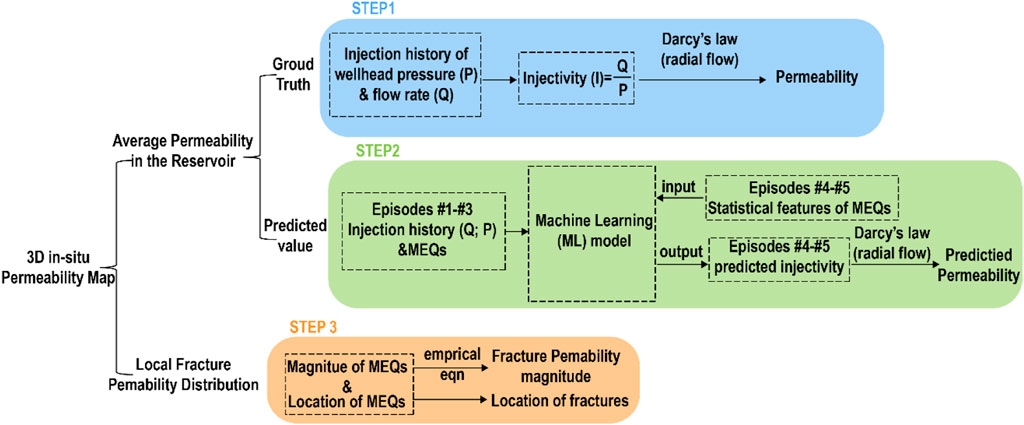
FIGURE 1. Logic chart and steps to create mean permeabilities and a permeability map.

Results

Deterministic permeability: Injection history data of pressure (red) and flow rate (blue) for the five stimulation episodes are shown in Figure 2A1–E1. Orange symbols represent the shortest distance of the seismic events from the injection well, with the symbol size scaling with the magnitude of individual MEQs for each episode correspondingly. Figure 2A2–E2 show the time histories of deterministic injectivity (light green line) and cumulative number of seismic events (orange line) for each episode. The deterministic injectivity is evaluated directly from the ratio of wellhead pressure and flow-rate histories. To convert the injectivity to average reservoir permeability, we assume that 1) fluid flows across the formation quasi-radially from the injection wellbore to an external migrating boundary and 2) the MEQs are partitioned between those resulting from changes in effective stress (80% assumed) and those beyond this region resulting from changes in total stress (20% assumed). Thus, the activated reservoir is confined to a volume that only contains fractures (MEQs) reactivated by fluid percolating from the injection (80% of the events), but this stimulated volume grows with time as the external cylindrical contour migrates as more distant MEQs occur. Thus, this migrating cylindrical envelope is estimated from the cumulative frequency of MEQs-with-radius and capped where cumulative frequency is 0.8.

FIGURE 2

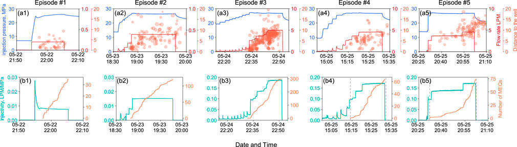
FIGURE 2. Seismic and injection information of the collab stimulation experiment (A1–A5) shows the injection history of the five stimulation episodes (blue line shows wellhead pressure and red line shows the flow rate) and the distance from MEQs to the injection well (orange symbols). Symbol sizes represent the MEQ magnitude. (B1–B5) shows the ground truth of injectivity history (light green lines) and the cumulative number of MEQs that occurred (orange line) of the five stimulation episodes, respectively. The dashed line shows the periods from the first MEQ which happened to well shut-in during episodes #4 (b4) and #5 (b5).

Figure 3A shows the histogram of the number of MEQs to the shortest distance of seismic events from the well for episode #4 at time T, and the cumulative frequency of MEQs (orange line) is calculated. The flow radius is then estimated where the cumulative frequency is 0.8 (gray line). The evolution of the flow radius can be estimated by time following the same strategy, and flow radius versus time for episode #4 and episode #5 are shown in Figures 3B,C. What is clear from this is that the effective radius of flow migrates monotonically outward during the two latter experiments. The radius is zero before any seismic events occur and grows upon their occurrence. This zone grows to 7.5 m at the end of episode #4 and ∼12 m for episode #5, suggesting a continuous flow pathway between injection and production wells.

FIGURE 3

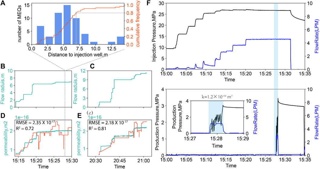
FIGURE 3. Deterministic permeability calculation and validation. (A) Illustration figure shows the flow radius estimated by the cumulative frequency of MEQs of 0.8 at the time T. Figure (B) and (C) show the evolution of the flow radius for episodes #4 and #5. (D) and (E) show the ground truth (light green line) and ML-predicted (orange line) permeabilities for episodes #4 and #5. (F) Top: pressure (black line) and injection flow rate (blue line) histories for episode #4. Bottom: pressure (black line) and flow rate (blue line) histories of the production well for episode #4. Insert figure shows the zoom in of the light blue shade area, where permeability is calculated and further used to validate the ground truth of permeability calculated by injectivity based on the cylindrical flow geometry.

We estimate the average permeability from the injectivity by presuming the radial flow from the 10 m-long borehole with interior and exterior pressure boundary conditions fixed to those of the injection and production well, respectively, as, $\mathrm{k}=\mathit{I}\mathit{\mu }\mathit{ln}\left(\mathit{r}/\mathit{r}\right)\mathit{2}\mathit{\pi }\mathit{h}$, where $\mathit{k}$ is the average permeability (m²); µ is the viscosity of water (8.9×10^–4 Pa·s); and r is the estimated radius of the cylindrical volume (m), which is derived from the migration of MEQs during the experiment. ${\mathit{r}}_{\mathbf{0}}$ is the interior/injection wellbore radius (0.048 m). This represents an approximation of the geometric correction for flow that is likely heterogeneous with azimuth but is considered uniform. The deterministic permeability for episodes #4 and #5 is represented by light green lines in Figures 3D,E. Figure 3F shows the well pressure (black line) and flow rate (blue line) histories for the injection well (top) and the production well (bottom) in episode #4. The flow rate was observed to fluctuate for a minute at the production well, highlighted by blue shaded area, which indicates that fluid has propagated to the production well. The permeability during this short period can be estimated using Darcy’s law, $\mathit{k}=\frac{\mathit{d}\mathit{q}\mathbf{\mu }\mathbf{L}}{\mathbf{A}\mathbf{d}\mathbf{p}}$, where dq (1.68 LPM) is the difference in the average flow rate between the two wells, L is the distance from the injection to the production well (10 m), A is the cross-sectional area (π·($\frac{\mathbf{10}}{\mathbf{2}}$)² m²), and dp (25.14 Mpa) is the average pressure difference between the two wells. The resultant permeability is 1.2 $\times {\mathbf{10}}^{-\mathbf{16}}{\mathrm{m}}^2$, which is close to our estimation of 2 $\times {\mathbf{10}}^{-\mathbf{16}}{\mathrm{m}}^2$ at the same time (T) based on the cylindrical flow geometry. This further confirms that the assumption of ∼80% of seismic events directly induced by effective stress (direct contact with elevated fluid pressures) is reasonable.

ML predicted the average permeability in the reservoir. An ML model is built using the data from the first three episodes #1–#3 with ∼450 MEQs and ∼2.5 h of well stimulation (training data). This consists of nine statistic features of the seismic data calculated over a small, moving time window, labeled by injectivity over the same time window. One time window corresponds to a minute. First, 80% of the training dataset will be used to train the model, and the rest of the 20% will be used to quantify whether the model is overfitting. Hyperparameters are set by fivefold cross-validation, and the best model is chosen using the root mean squared error (RMSE) as an evaluation metric. The step-by-step description of data analysis and machine learning methods is documented in the Methods section. It must be noted that the training data can be the dataset of any single episode of the three or few episodes that occurred before the predicted episode. For example, to estimate injectivity in episode #4 (testing data), the training dataset can comprise episode #3 only or all three episodes from #1 to #3. We run 6 tests in total to find out the optimum train dataset and input features to predict injectivity for episode #4 and #5. A total of nine statistic features of MEQs produce 511 combination possibilities. Each combination of features will be applied to build an ML model for every single test, and the best model for each test is quantified when R2 is closest to 1, using the difference between the deterministic and predicted features in each episode. These models are selected for each of the best with its input features, R2, RMSE, and hyperparameters, as shown in Table 1.

TABLE 1

TABLE 1. Input features and hyperparameter performance.

We show the most accurate predicted injectivity from the ML model (red line) in episode #4 (Figure 4A) and episode #5 (Figure 5A), and compare it with the deterministic injectivities (blue line). ML is applied to predict injectivity during the period starting from the first MEQ that occurred to the well shut in (the time between two dashed lines in Figure 2B4,B5). The scatter plots in Figure 4B and Figure 5B show the ground truth of average injectivity versus machine learning estimations of injectivity using only the statistics of MEQs. A perfect model would follow the gray dashed line. RMSE and R2 are calculated for each project, with RMSE = 0.056 and R2 = 0.63 for episode #4 and RMSE = 0.017 and R2 = 0.69 for episode #5. This, together with the general concurrence in the time histories, confirms the excellent agreement between the ground truth and ML predicted injectivities. Importantly, this injectivity is predicted purely based on the training of the ML algorithm against injectivity-vs-MEQ histories over episode #3 to predict injectivity over episodes #4 and #5 from the MEQs alone. These predictions are derived purely from the statistical features of the seismic events from a history of injectivity that the model has never seen. We emphasize that there is no past nor future information considered when making such a prediction. Each prediction uses only the statistical features of seismic events within a single moving window. Thus, we can predict the corresponding history of injectivity in episode #4 from the seismic catalog alone.

FIGURE 4

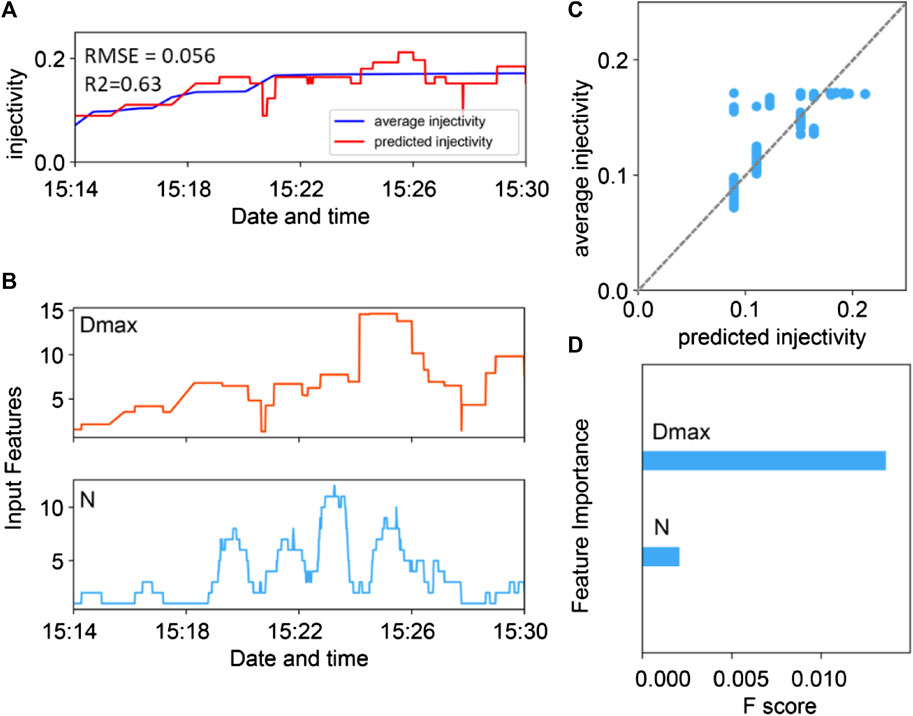
FIGURE 4. Predicted injectivity of episode #4. (A) Average injectivity by the time moving window (blue line) and predicted injectivity (red line) from the ML model in episode #4. (B) The input features are used to construct the machine learning model. (C) Average permeability vs predicted permeability in episode #4. (D) The importance of input features.

FIGURE 5

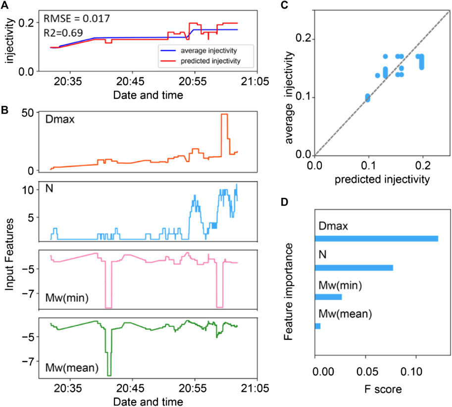
FIGURE 5. Predicted injectivity of episode #4. (A) Average injectivity by time moving window (blue line) and predicted injectivity (red line) from the ML model in episode #5. (B) The input features used to construct the machine learning model. (C) Average permeability vs predicted permeability in episode #5. (D) The importance of input features.

As an ML algorithm makes explicit decisions based on the values of the features, a trained XGBoost model can automatically calculate the importance of the predictive features and therefore enables us to gain physical understanding of the problem. An F-score is used to evaluate the importance of each input feature, which implies the relative contribution of the corresponding feature to the model, calculated by taking each feature’s contribution for each tree in the model. A higher value of this metric, when compared to another feature, implies it is more important for generating a prediction. The evolution of the predictive key features for episodes #4 and #5 are shown in Figure 4C and Figure 5C, and their feature importance is presented using the F-score by plots shown in Figure 4D and Figure 5D, respectively. For the estimates of injectivities, the top two features correspond to the maximum distance from MEQs to the injection well, and the number of the MEQs that occurred within a time window.

We then convert the predicted injectivity to a mean permeability by incorporating an approximated flow geometry and an estimated magnitude of the migrating flow radius as in step 1. The evolution of the predicted average permeability for episodes #4 and #5 is shown as an orange line in Figures 2D,E for easy comparison. We observe that both deterministic and predicted average permeability gradually increase to a maximum until well shut in. The well agreement of deterministic and predicted average permeability curves confirms the accuracy of the ML model with RMSE = 2.35 ×10^–17 and R² = 0.72 for episode #4 and RMSE = 2.18 ×10^–17 and R² = 0.81 for episode #5.

3D in situ permeability map and permeability structure: Physics-inspired models of MEQs are applied to define the spatial evolution of permeability on individual fractures/MEQs over episodes #4 and #5. The matrix is effectively impermeable (set to 10^–19 m²; Neupane et al., 2019) with a local fracture permeability created by MEQs determined from Equation 10 and represented by the data-point cloud. The dark blue symbols in Figure 6A,B represent the fracture permeability created by MEQs from initiation to termination of the respective injection episodes #4 and #5. The predicted fracture permeability is shown spatially and indexed by color intensity. Symbol size reflects the magnitude of the related seismic events. Fracture permeability created by all MEQs during the entire stimulation episode are shown in Figure 6C (from #1–#4) and Figure 6D (#1–#5). The outer contour of the cylindrical volume follows the extent of water migration, with the color indicating average reservoir permeability predicted by the ML model. The stimulated zone of the enhanced fracture permeability migrates radially outward from the injection well (red line) preferentially toward the production wells (green line). This suggest that new and reactivated fractures are propagated from the injection well toward the production well that is azimuthally focused toward the production well. A plan view of the 3D permeability map predicted for all episodes (Figure 7) shows the form of fracture propagation from the injection to the production well and identifies the possible fluid path. Symbols colored from light to dark green show the spatial permeability that was created from episodes #1 to #5 with a symbol size indicating the MEQ magnitude. The color transition from light to dark is consistent with the fluid path created from the injection to the production well (Figure 7A) and propagates from a shallower to deeper position in the reservoir (Figure 7B). The 3D in situ permeability map shown in Figure 5C,D integrates both average reservoir permeability and fracture permeability distribution. Importantly, the map defines both the spatial distribution of permeability and the magnitude and distribution of the heat transfer area—a key factor in defining the efficiency of heat exchange within a prospective geothermal reservoir. The largest permeability enhancement is represented by the denser zone of fractures. The insights gained through the application of these methods can be incorporated into conceptual models and utilized for planning exploration and development strategies in operating geothermal fields.

FIGURE 6

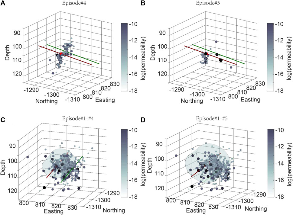
FIGURE 6. Spatial in situ permeability map. (A) and (B) show spatial permeability distribution for episodes #4 and #5 only. (C) and (D) show local fracture permeability cumulated from episodes #1–#4 and #1–#5. The outer contour of the cylindrical volume follows the extent of water migration with the color indicating average reservoir permeability predicted from the ML model at the end of episodes #4 and #5. Red and blue lines represent injection and production well, respectively.

FIGURE 7

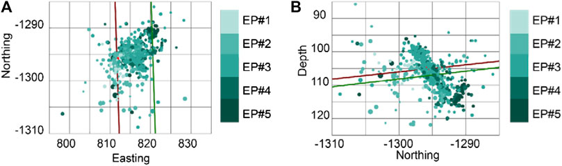
FIGURE 7. Top view (A) and side view (B) of the 3D permeability map show the fracture propagation and potential fluid paths.

FIGURE 8

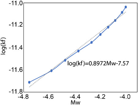
FIGURE 8. Log–log plot of the fracture permeability versus the seismic moment magnitude. Data from Li et al. (2021).

We average the evolving spatial distribution of permeability recovered from Equation 10 (step 3) to compare it against the average permeability recovered from the previous steps. We mesh a 20×20×10 m cube that contains a 10-m radius cylinder and discretize the volume using a 0.1 m grid. Each calculated fracture permeability value is then assigned into the mesh block based on its location. If several fractures are in the same mesh block, then the largest (most dominant) of the fracture permeabilities is selected. Mesh blocks without fractures are assigned as a matrix permeability of 10⁻¹⁹ m². We arithmetically average and volume-weight the permeability across all mesh blocks. The cross comparison of the average permeability by different methods at the end of episodes #4 and #5 are shown in Table 2. Permeability between two wells for episode #4 is calculated by Darcy’s law as shown in Figure 3E-insert. No data on the flow rate and the pressure at the production well for episode #5 have been collected, thus permeability estimated using this method is missing. It is observed that the average permeability estimated by the physics-inspired model is slightly higher than that of the other methods. This may be because the model estimates the arithmetical mean of both the fracture and matrix permeability without considering if fractures created by MEQs are connected to the main fluid path, and thus there is the possibility of overestimation in the average permeability. The deterministic permeabilities for episodes #4 and #5 recovered from the injectivity ground truth (Step 1) are in the magnitude of average permeabilities estimated from the fracture permeability maps (Step 3)—indicating that fracture permeabilities may be directly constrained from MEQs and based on the moment’s magnitude.

TABLE 2

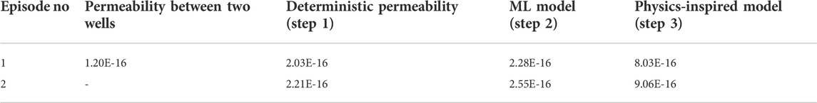
TABLE 2. Cross validation of permeability by different methods.

Discussion

Our hybrid ML methods applied to this EGS-Collab stimulation experiment can define an inherent correlation between MEQs and well injection history. Based on ML methods, injectivity is predicted from the statistical features of the seismic events, corresponding to a history of injectivity that the model has never seen. This is accomplished by training the ML model in early episodes of observation and predicting over the final two episodes. The average permeability of the fractured reservoir is then calculated from injectivity, using a geometric correction of the steady state. This causality between injectivity/permeability and MEQs is then used to develop a physics-inspired model linking permeability evolution to MEQ magnitude. This relies on the parallel plate analog linking permeability to dilation and is then supplemented by laboratory observations scaling dilation to the equivalent MEQ magnitude. These data are then scaled to link individual MEQs of known magnitude and location to define incremental changes in permeability in both space and in time. This pointwise distribution of permeability is then used to define a map of permeability structure and then averaged to recover the mean permeability evolution. This prediction closely matches the measured ground truth of the ensemble permeability recovered from this unusually well-constrained injection experiment. The promising approach to quantify the evolution of permeability as a function of observable MEQs proves a valuable tool in the characterization of reservoirs with the potential to visualize the evolution of potential fluid flow paths, the generation of reactive/heat-transfer surface area, and the capability of further constraint using superimposed signals, say of tracer response. Challenges for the application of this method to a larger scale include dealing with much noisier data, applying longer injection histories, and data on operation under various conditions need to be collected as a database to build ML models and to evaluate and improve accuracy.

Domain knowledge plays an essential role in choosing statistic features in ML models. We chose nine statistic features in the model to eliminate the dependence of injectivity on 1) number of MEQs, 2) magnitude of MEQs, and 3) the distance of MEQs from the injection well in the regression problem. The results illustrate that the distance of MEQs from the injection well is the dominant feature in predicting injectivity, followed by the number of MEQs and then the magnitude of MEQs. It should also be mentioned that the success of the supervised ML approach is heavily dependent on the training dataset used. Our results show that using the data of episode #3 only to predict episodes #4 or #5 is much more accurate than using all three episodes. This is because flow rates after episode #3 were more than ten times higher than those used in prior stimulations (episodes #1–2) with a similar injection pressure, which led to tenfold increased injectivity. If we choose episodes #1–3 instead of episode #3 only, this will include ∼78% (110 out of 140 min) of injectivity data and ∼33% (150 out of 450 seismic events) of MEQs data irrelevant for higher injectivities like the later episodes. This undoubtedly decreases the accuracy in prediction. Therefore, choosing the dataset with similar characteristics delivers better prediction than using the bigger but irrelevant dataset.

Conclusion

We show that hybrid ML methods applied to this EGS-Collab stimulation experiment are capable of defining an inherent correlation between MEQs and well-injection history—specifically, the injectivity, defined as the ratio of the instantaneous flow rate and the wellhead pressure. This is accomplished by training the ML model in early episodes of observation (episodes #1–#3) and predicting over the final two episodes (#4). Thus, injectivity is predicted from the statistical features of the seismic events from a history of injectivity that the model has never seen. The average permeability of the fractured reservoir is then calculated from injectivity, using a geometric correction of the steady state—which is then assumed as the ground truth. This causality between injectivity/permeability and MEQs is then used to develop a physics-based model linking permeability evolution to the MEQ magnitude. This relies on the parallel plate analog linking permeability to dilation and then supplemented by laboratory observations scaling dilation to the equivalent MEQ magnitude. These data are then scaled to link individual MEQs of known magnitude and location to define incremental changes in permeability in both space and time. This pointwise distribution of permeability is then used to define a map of permeability structure and then averaged to recover the mean permeability evolution. This prediction closely matches the measured ground truth of the ensemble permeability recovered from this unusually well-constrained injection experiment. The promising approach to quantify the evolution of permeability as a function of observable MEQs proves a valuable tool in the characterization of reservoirs with the potential to visualize the evolution of potential fluid-flow paths, the generation of reactive/heat-transfer surface area, and the capability of further constraint using superimposed signals, say of tracer response. Challenges for the application of this method to a larger scale include dealing with much noisier data, applying longer injection histories, and data on operation under various conditions need to be collected as a database to build ML models and to evaluate and improve accuracy.

Methods

Data analysis and machine learning methods

1) Data arrangement: In this project, well injection data are continuously recorded every second, and a seismic catalogue is recorded for each seismic event, which is not continuous in time-like well data. We start by creating files of the well injection history and seismic catalogue with a common time base. We then scan both well data and seismic data using the same moving time windows, and compute statistic features of seismic data and average injectivity for each of these windows. We define nine features (the statistic features of seismic data) for the ML model including maximum seismic magnitude (Mwmax), minimum seismic magnitude (Mwmin), average seismic magnitude (Mwmean) within each window, maximum value (Dmax), minimum value (Dmin), and average value (Dmean) of distance from seismic events to the injection well; estimated flow radius (R); the number of seismic events within each window (N); and the cumulative number of seismic events from the beginning to the current window (Ntotal). Thus, each line of the database contains the variables and the corresponding average injectivity during the same time. The time series of variables is then labeled with the injectivity correspondingly. The size of the time moving window is picked for a minute, and each time window moves forward for a second. We build variables and the corresponding labels, and then add the resulting list of labeled features to the database at each time increment. Finally, each line of the dataset i is a list {x_i¹, x_i², x_i³ … x_iⁿ, y_i}, with x_iⁿ the n th feature of the i-th time window of the seismic data, n is the total number of features, and y_i is the average injectivity during the same time moving window.

2) Train–validate–test split: We aim to use the ML model to predict injectivity in episodes #4 and #5. The training dataset can be the dataset of one single episode or the combination of a few episodes that occurred before the predicted episode. For example, to estimate injectivity in episode #4 (testing data), the training dataset can be episode #3 only or episodes #1 to #3. The details of training data and testing data are given in Table 1. As the database has time series features of the seismic data and the corresponding average injectivity, the train–validate split must be of two continuous datasets in time, not a random split. Here, we use the first 80% of the training dataset to construct the ML model and the rest 20% of the training dataset for validating the model.

3) Choose the features: The dataset is now composed of nine features describing the seismic data versus the time moving window. Our goal is to predict the injectivity based on the given features. The features can be any combinations of these nine features, which results in 511 possibilities.

4) Training and tuning the ML model: We build trail models using both the train and test datasets with default hyperparameters and evaluate the model performance by the root mean square error (RMSE). Then hyperparameters are tuned on the training dataset to minimize the RMSE using cross-validation. We tune hyperparameters in the model, and all the combinations of hyperparameters with specific values in a range are tested to guarantee the optimal solution (max depth [1,10], min child weight [1,10], eta [0.005,0.5], subsample [0,1], and colsample by tree [0,1]. Five-fold cross-validation is applied for each combination of hyperparameters, where the training dataset is split into 5 folds and iteratively keeps one of the folds for test purposes and returns an RMSE score. The optimum hyperparameters are chosen with the minimum RMSE. Then, the model is checked by the validation dataset to make sure this model is not overfitting. The final model is then created using the training and validation datasets with updated hyperparameters.

5) Make prediction: We can now make predictions using the best model (final model). The combination of features will be selected and then input into the best model to predict injectivity. The predicted data will be compared with the ground truth of injection to assess the performance of the model.

6) Feature importance: We can look for the best features identified by our model to try to understand how the model reached its estimations. Here, we apply the feature importance type as “gain,” which implies the relative contribution of the corresponding feature to the model calculated by taking each feature’s contribution for each tree in the model. A higher value of this metric when compared to another feature implies that it is more important for generating a prediction.

Linking seismic magnitude with the fracture permeability using an empirical equation.

Here, we develop a new method to link MEQs and a fracture permeability change during hydraulic stimulation of a fractured reservoir. First, a simple configuration of hydro-shear failure is assumed to be generated by microearthquakes (MEQs) during stimulation, with a shear displacement of u (m) uniformly applied to a square fracture plane of fracture length L (m). The fracture area A (m²) is then simply defined as follows

$\mathit{A}={\mathit{L}}^{\mathbf{2}}.(1)$

It has been demonstrated that the fracture length can be estimated by an aperture using an exponent relationship as follows (Ishibashi et al., 2016):

$\mathit{b}=\mathit{\alpha }{\mathit{L}}^{\mathit{\beta }},(2)$

where $b$ is the fracture aperture $\left(m\right)$, and $\alpha$ and $\beta$ are the coefficients that link the fracture aperture and length. Permeability ${\mathit{k}}_{\mathit{f}}\left(m^2\right)$ can be estimated from the fracture aperture using the cubic law as follows:

${\mathit{k}}_{\mathit{f}}=\frac{{\mathit{b}}^{\mathbf{2}}}{\mathbf{12}}.(3)$

Based on the concept of the seismic moment ${\mathit{M}}_{\mathbf{0}}$ (Scholz, 2019),

${\mathit{M}}_{\mathbf{0}}=\mathit{A}\mathit{G}\mathit{u},(4)$

where G is the shear modulus of the reservoir rock, usually of the order of 30 GPa (McGarr, 2014).

Seismic moment can be converted to an MEQ magnitude ${\mathit{M}}_{\mathit{w}}$ using the following equation:

$\mathit{log}{\mathit{M}}_{\mathbf{0}}=\mathbf{1.5}{\mathit{M}}_{\mathit{w}}+\mathbf{9.1},(5)$

(Hanks and Kanamori, 1979).

The seismic moment related to fracture area can be expressed as follows:

$\mathit{log}{\mathit{M}}_{\mathbf{0}}=\mathbf{1.5}\mathbf{log}\left(\mathit{A}\right)+\mathbf{6.09},(6)$

(Leonard, 2010).

If we combine Equations (1–3) and (5–6), we can successfully link the fracture permeability with the seismic magnitude:

${\mathit{k}}_{\mathit{f}}=\frac{{\mathit{\alpha }}^{\mathbf{2}}}{\mathbf{12}}{\mathbf{10}}^{\mathit{\beta }\left(\mathbf{0.5}{\mathit{M}}_{\mathit{w}}+\mathbf{1}\right)}.(7)$

Assuming ${\mathit{\alpha }}_{\mathbf{1}}=\frac{{\mathit{\alpha }}^{\mathbf{2}}}{\mathbf{12}}$, taking the logs of both sides of Equation 7 yields

$\mathbf{log}\left({\mathit{k}}_{\mathit{f}}\right)=\mathit{\beta }\left(\mathbf{0.5}{\mathit{M}}_{\mathit{w}}+\mathbf{1}\right)+\mathbf{log}\left({\mathit{\alpha }}_{\mathbf{1}}\right).(8)$

To determine the coefficients ${\alpha }_1$ and $\beta$ for the reservoir injection here (EGS-Collab project), we used experimental data that concurrently measured the aperture and shear displacement during slip on laboratory faults as the pore pressure was incremented due to fluid injection (Figure 1A of Li et al., 2021). These are the same reservoir rocks as in the field experiment. The seismic moment is then calculated from measured reactivation displacement (Equation 4), and permeability is evaluated from the measured aperture (Equation 3)—both independently. Substitution of multiple correlated values of permeability $k_f$ and moment $M_w$ into Equation 8 then yields the coefficients ${\alpha }_1$ and $\beta$. The results for change in fracture permeability $k_f$ as a function of seismic moment $M_w$ are shown in Figure 7, with regression defining the fitting parameters as

$\mathbf{log}\left({\mathit{k}}_{\mathit{f}}\right)=\mathbf{0.8972}{\mathit{M}}_{\mathit{w}}-\mathbf{7.57},(9)$

and therefore, from Eq. 8 ,we obtain ${\mathit{\alpha }}_{\mathbf{1}}=4.6\times {10}^{-10}$ and $\beta =1.7584$.

MEQs are then linked to the fracture permeability change during the hydraulic stimulation as follows:

$\mathbf{k}=\mathbf{4.6}\times {\mathbf{10}}^{-\mathbf{10}}\times {\mathbf{10}}^{\mathbf{0.8972}{\mathbf{M}}_{\mathbf{w}}+\mathbf{1.7584}}.(10)$

EGS-collab

CSM—Y.S. Wu, J. Miskimins, P. Winterfeld, K. Kutun; DOE, L. Boyd, Z. Frone, E. Metcalfe, A. Nieto, S. Porse, and W. Vandermeer; J. McLennan, the University of Utah; INL, R. Podgorney, G. Neupane, LBNL; J. Ajo-Franklin, P.J. Cook, P.F. Dobson, C.A. Doughty, Y. Guglielmi, M. Hu, R.S. Jayne, K. Kim, T. Kneafsey, S. Nakagawa, G. Newman, P. Petrov, M. Robertson, J. Rutqvist, M. Schoenball, E.L. Sonnenthal, F.A. Soom, C. Ulrich, C.A. Valladao, T. Wood, Y.Q. Zhang, Q. Zhou; LANL, L. Huang, Y. Chen, B. Chi, Z. Feng, L.P. Frash, K. Gao, E. Jafarov, S. Karra, N. Makedonska, W. Pan, R. Pawar, N. Welch; LLNL, P. Fu, R.J. Mellors, J.P. Morris, M.M. Smith, D. Templeton, H. Wu; Mattson Hydrology LLC: E. Mattson; NETL—J. Moore, S. Brown, D. Crandall, P. Mackey, T. Paronish, S. Workman; NREL, B. Johnston, K. Beckers, J. Weers; ORNL, Y. Polsky, Monica Maceira, Chengping Chai; Penn State—D. Elsworth, K.J. Im, Z. Li, C.J. Marone, E.C. Yildirim; PNNL, A. Bonneville, J.A. Burghardt, J. Horner, T.C. Johnson, H. Knox, J. Knox, B.Q. Roberts, P. Sprinkle, C.E. Strickland, J.N. Thomle, V.R. Vermeul, M.D. White; Stanford—M.D. Zoback - A. Singh; Stanford—M.D. Zoback - A. Singh; Stanford—R.N. Horne, K. Li, A. Hawkins, Y. Zhang; Rice University—Jonathan Ajo-Franklin; ResFrac - M.W. McClure; South Dakota School of Mines and Technology—W. Roggenthen, C. Medler, N. Uzunlar, Carson Reimers; SNL, D. Blankenship, M. Ingraham, J. Pope, P. Schwering, A. Foris, DK King, J. Feldman, M. Lee, J. Su; SURF, T. Baumgartner, J. Heise, M. Horn, B. Pietzyk, D. Rynders, G. Vandine, D. Vardiman; Subs, Thomas Doe, TDoeGeo Rock Fracture Consulting; Golder Associates Inc; the University of Oklahoma - A. Ghassemi, Dharmendra Kumar, Varahanaresh Sesetty, Alex Vachaparampil; the University of Wisconsin-Madison—H.F. Wang, Hiroki Sone, Kate Condon, and Bezalel Haimson.

Data availability statement

The raw data supporting the conclusions of this article will be made available by the authors, without undue reservation.

Author contributions

DE conceived the study; ZL conducted data analyses, and prepared the manuscript and figures. CW contributed to the interpretation of all the results. All authors discussed the results and implications, and revised the manuscript.

Acknowledgments

This work is a partial result of support from the DOE EGS Collab Project: Stimulation Investigations for Geothermal Modeling, Analysis, and Validation. This support is gratefully acknowledged. We acknowledge support from DOE-GTO under the EGS-Collab Project and Project DE-EE0008763. In addition DE acknowledges support from the G. Albert Shoemaker endowment.

Conflict of interest

The authors declare that the research was conducted in the absence of any commercial or financial relationships that could be construed as a potential conflict of interest.

Publisher’s note

All claims expressed in this article are solely those of the authors and do not necessarily represent those of their affiliated organizations, or those of the publisher, the editors, and the reviewers. Any product that may be evaluated in this article, or claim that may be made by its manufacturer, is not guaranteed or endorsed by the publisher.

References

Bauer, J. F., Krumbholz, M., Meier, S., and Tanner, D. C. (2017). Predictability of properties of a fractured geothermal reservoir: The opportunities and limitations of an outcrop analogue study. Geotherm. Energy 5 (1), 24–27. doi:10.1186/s40517-017-0081-0

CrossRef Full Text | Google Scholar

Bauer, J. F., Krumbholz, M., Luijendijk, E., and Tanner, D. C. (2019). A numerical sensitivity study of how permeability, porosity, geological structure, and hydraulic gradient control the lifetime of a geothermal reservoir. Solid earth. 10 (6), 2115–2135. doi:10.5194/se-10-2115-2019

CrossRef Full Text | Google Scholar

Cheng, Q., Wang, X., and Ahmad, G. (2019). Numerical simulation of reservoir stimulation with reference to the Newberry EGS. Geothermics 77, 327–343. doi:10.1016/j.geothermics.2018.09.011

CrossRef Full Text | Google Scholar

Frash, L. P., Carey, J. W., and Welch, N. J. (2019b). “EGS collab experiment 1 geomechanical and hydrological properties by triaxial direct shear,” in Proceedings of the 44th Workshop on Geothermal Reservoir Engineering, California, 11-13 Feb. 2019.

Google Scholar

Fridleifsson, I. B. (2008). Present status and potential role of geothermal energy in the world. Renew. Energy 20 (25), 34–39. doi:10.1016/0960-1481(96)88816-1

CrossRef Full Text | Google Scholar

Fu, P., Kneafsey, T. J., Morris, J. P., and White, M. D. (2018). “Predicting hydraulic fracture trajectory under the influence of a mine drift in EGS Collab experiment I,” in Proceedings of the 43rd Workshop on Geothermal Reservoir Engineering, February 12–14, 2018.

Google Scholar

Fu, P., Schoenball, M., Morris, J. P., Ajo-Franklin, J., Knox, H., Kneafsey, T., et al. (2019). “Microseismic signatures of hydraulic fracturing: A preliminary interpretation of intermediate-scale data from the EGS collab experiment 1,” in Proceedings of the Stanford Geothermal Workshop 44th Annual, CA, United States, 11-13 Feb. 2019.

Google Scholar

Hanks, T. C., and Kanamori, H. (1979). A moment magnitude scale. J. Geophys. Res. 84, 2348–2350. doi:10.1029/jb084ib05p02348

CrossRef Full Text | Google Scholar

Ishibashi, T., Watanabe, N., Asanuma, H., and Tsuchiya, N. (2016). Linking microearthquakes to fracture permeability change: The role of surface roughness. Geophys. Res. Lett. 43 (14), 7486–7493. doi:10.1002/2016gl069478

CrossRef Full Text | Google Scholar

Kneafsey, T. J., Dobson, P., Blankenship, D., Morris, J., Knox, H., Schwering, P., et al. (2018). “An overview of the EGS collab project: Field validation of coupled process modeling of fracturing and fluid flow at the sanford underground research facility, lead, SD,” in Proceedings of the 43rd Workshop on Geothermal Reservoir Engineering, California, 12-14 Feb. 2018. paper SGP-TR-213. Preprint at https://pangea.stanford.edu/ERE/pdf/IGAstandard/SGW/2018/Kneafsey.pdf.

Google Scholar

Kneafsey, T. J., Blankenship, D., Knox, H. A., Johnson, T. C., Ajo-Franklin, J. B., Schwering, P. C., et al. (2019). “EGS Collab project: Status and progress,” in Proceedings of the 44th Workshop on Geothermal Reservoir Engineering, California, 11-13 Feb. 2019.

Google Scholar

Kushnir, A. R. L., Heap, M. J., and Baud, P. (2018). Assessing the role of fractures on the permeability of the Permo-Triassic sandstones at the Soultz-sous-Forêts (France) geothermal site. Geothermics 74, 181–189. doi:10.1016/j.geothermics.2018.03.009

CrossRef Full Text | Google Scholar

Laubach, S. E., Olson, J. E., and Gross, M. R. (2009). Mechanical and fracture stratigraphy. Am. Assoc. Pet. Geol. Bull. 9311, 1413–1426. doi:10.1306/07270909094

CrossRef Full Text | Google Scholar

Li, Z., Elsworth, D., and Wang, C. (2021). Constraining maximum event magnitude during injection-triggered seismicity. Nat. Commun. 121, 1528–1529. doi:10.1038/s41467-020-20700-4

PubMed Abstract | CrossRef Full Text | Google Scholar

McGarr, A. (2014). Maximum magnitude earthquakes induced by fluid injection. J. Geophys. Res. Solid Earth 119 (2), 1008–1019. doi:10.1002/2013jb010597

CrossRef Full Text | Google Scholar

Neupane, G. H., Podgorney, R. K., Huang, H., Mattson, E. D., Kneafsey, T. J., Dobson, P. F., et al. (2019). EGS Collab Earth modeling: Integrated 3D model of the testbed. Idaho Falls, ID (United States): Idaho National Lab INL.

Google Scholar

Schoenball, M., Ajo-Franklin, J. B., Blankenship, D., Chai, C., Chakravarty, A., Dobson, P., et al. (2020). Creation of a mixed-mode fracture network at mesoscale through hydraulic fracturing and shear stimulation. JGR. Solid Earth 125 (12), e2020JB019807. doi:10.1029/2020jb019807

CrossRef Full Text | Google Scholar

Scholz, C. H. (2019). The mechanics of earthquakes and faulting. Cambridge, United Kingdom: Cambridge University Press.

Google Scholar

Williams, C. F., Reed, M. J., Mariner, R. H., DeAngelo, J., and Peter Galanis, S. (2008). Assessment of moderate-and high-temperature geothermal resources of the United States. USA: Geological Survey US.

Google Scholar