 Jizhong Yang
 Jian Zhou
 Heng Zhang
 Tuanwei Xu
 Dimin Deng
 Jianhua Geng
95% of researchers rate our articles as excellent or good
Learn more about the work of our research integrity team to safeguard the quality of each article we publish.
Find out more
ORIGINAL RESEARCH article
Front. Earth Sci. , 11 January 2023
Sec. Solid Earth Geophysics
Volume 10 - 2022 | https://doi.org/10.3389/feart.2022.1018116
This article is part of the Research Topic Advances and Applications of Distributed Optical Fiber Sensing (DOFS) in Multi-scales Geoscience Problems View all 13 articles
The harsh and extreme environmental and near surface conditions of the Tibetan Plateau have limited the conventional electrical-based seismic instruments from obtaining high-quality seismic data through long-term and continuous observations, setting challenges for environmental seismology study and natural hazard monitoring in this area. Distributed acoustic sensing (DAS) is an emerging technique based on optical fiber communication and sensing. It provides a possible solution for subsurface imaging in extreme conditions at high spatiotemporal resolution by converting fiber-optic cables into dense seismic strainmeters. We deploy two survey lines with armored optical fiber cables in the Yigong Lake area, Southeastern Tibetan Plateau, to record ambient noise for a week. The DAS interrogator is specifically designed in a portable size with very low power consumption (25 W/h). Hence, we can use a 12V-DC battery for power supply to adjust the power limitation during the field recording. Ambient noise interferometry and multichannel analysis of surface waves are used to get 2D shear wave velocity profiles along the fiber paths. The results highlight the great potential of DAS for dynamic monitoring of the geological evolution of lakes and rivers in areas of extreme environments as in the Tibetan Plateau.
Seismic data acquisition is the foundation of data processing and interpretation in seismological research. High-quality seismic data may significantly improve the accuracy of geological understanding. Recently, seismologists have tried to use denser and denser observational networks to obtain high-spatiotemporal-resolution seismic data for a better knowledge of the Earth’s dynamic processes and monitoring of natural hazards (Karplus and Schmandt, 2018; Nishikawa et al., 2019; Kohler et al., 2020). Although conventional electrical seismic instruments can be deployed in most areas for seismological research, it is very challenging to meet the aims of long-term monitoring in harsh environments, such as the volcano, glaciers, and plateaus due to the high cost of deployment and maintaining.
Distributed acoustic sensing (DAS) is an emerging seismic measurement technique that benefits from the development of optical fiber communication and sensing. Typically, a DAS system is composed of a standard optical fiber cable and an interrogation unit (IU). The IU lights the fiber using short laser pulses and measures Rayleigh back-scattering (RBS) along the fiber through a form of coherent optical time domain interferometry. A phase shift in the RBS is caused by the compression or elongation along the fiber, which is proportional to axial strain along the cable. Thus, DAS is working as a dense network for dynamic strain measurements (Parker et al., 2014; Hartog, 2017). DAS has initially been used for downhole applications in oil and gas exploration (Mateeva et al., 2014; Daley et al., 2016; Lellouch and Biondi, 2021). Currently, it has been widely adapted to seismological investigations, such as earthquake detection (Lindsey et al., 2017; Jousset et al., 2018; Wang et al., 2018; Yu et al., 2019), near-surface characterization (Dou et al., 2017; Fang et al., 2020; Spica et al., 2020; Shao et al., 2022), observing oceanic and atmospheric phenomena (Lindsey et al., 2019; Sladen et al., 2019; Williams et al., 2019; Zhu and Stensrud, 2019; Shinohara et al., 2022), monitoring volcano and glacier (Booth et al., 2020; Walter et al., 2020; Klaasen et al., 2021; Nishimura et al., 2021), and so forth. For the most up-to-date review of DAS application in seismology, we refer the readers to Lindsey and Martin (2021).
In this study, we use DAS to record continuous ambient noise in the Yigong Lake area in Tibetan Plateau. Yigong Lake is a barrier lake in the Yigong village, Bome County, Nyingchi, Tibet, characterized by a high altitude, a weak geological foundation, and an active modern crustal movement. It is located in the southeast of the Tibetan Plateau, about 2,600 m above sea level and spanned about 20 square kilometers (Figure 1). The strong uplift of the Earth’s crust makes it the heaviest and wettest region on the Tibetan Plateau and prone to natural disasters such as landslides, avalanches, and debris flows. Historic records show that two giant landslides occurred in 1,900–2,000 resulting a deposit of total volume about 5
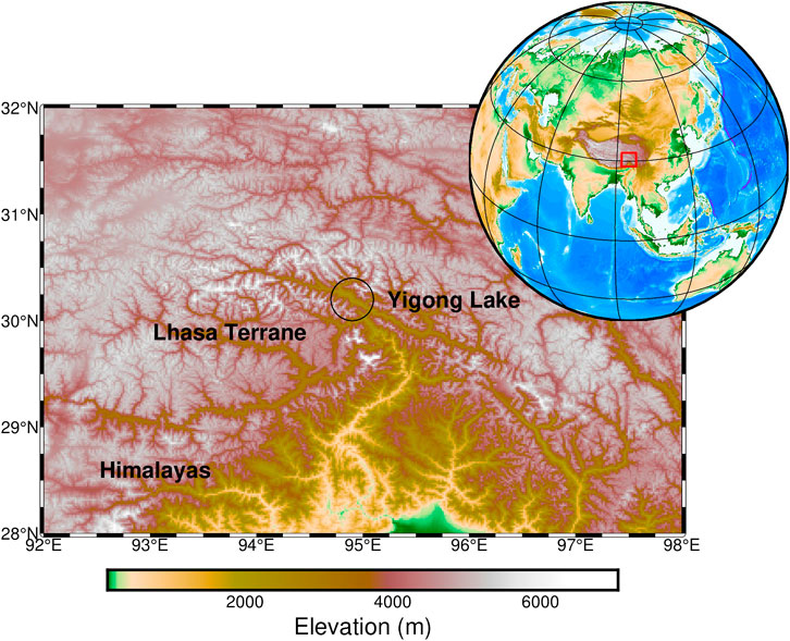
FIGURE 1. Geographic location and map overview.
In the following parts, we first introduce the field deployment of seismic data acquisition using DAS. Thereafter, seismic interferometry is applied to the pre-processed data to obtain the noise correlation functions (NCFs) following the workflow of Bensen et al. (2007). After extracting surface waves from NCFs, multichannel analysis of surface waves (MASW) (Park et al., 1999) is utilized to retrieve dispersion curves and invert the shear wave velocity. According to the variations of the shear wave velocity, the sedimentary thickness in the study area can be inferred. These results confirm the reliability of DAS in capturing data and performing near-surface characterization in extreme environments.
The ambient noise data acquisition is located between a highway and the Yigong Lake, as shown in Figure 2. In this area, it is not readily available to get access to the industrial power supply, and there is no facility room for equipment installation. To perform seismic data acquisition under such an extreme condition, the DAS IU is specially manufactured to have a portable size of 150 mm
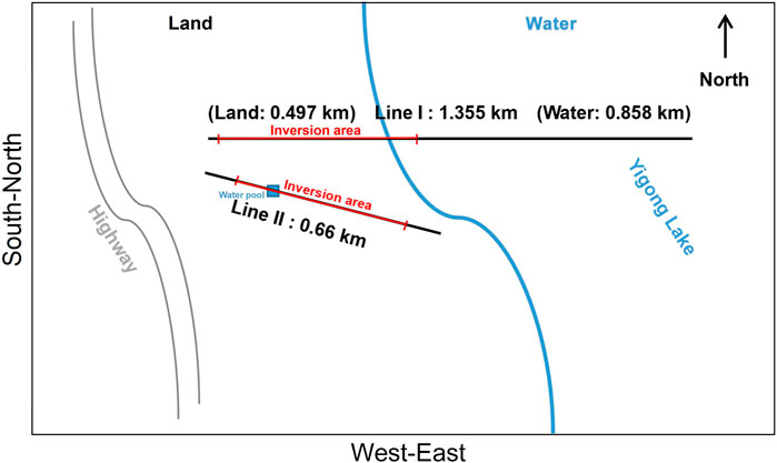
FIGURE 2. Schematic layout of the trenched optical fiber cables.
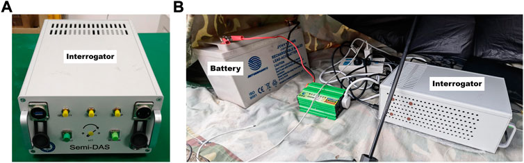
FIGURE 3. Photos for the interrogator in a front view (A) and the battery connection during field data acquisition (B).
DAS data were acquired during the local daytime from 10 a.m. to 7 p.m. on 28 October 2021 to 3 November 2021. The maximum continuous recording length is 8 h because of running out of battery power. We installed two trenched DAS arrays. The surface trenches, which are 10cm–20 cm deep, are dug with hand tools. The optical fiber cables were backfilled with excavated soil to ensure coupling between DAS and the ground, as shown in Figure 4A. Line I is 1.355 km long with 755 channels. A 0.497 km-long session of the line was settled on the ground while the rest of the line was deployed underwater across the Yigong Lake. This line was originally installed in April 2021, when the Yigong Lake is in the dry season so that we could easily get access to the lake bottom to deploy optical fiber cables. During the data acquisition time, the Yigong Lake is in the wet season and optical fiber cables are buried underwater. At the transition zone from the land to the water, parts of optical fiber cables are suspended in the air, as shown in Figure 4B. Consequently, the DAS data are discontinuously recorded during the test stage. After realizing this, we buried the suspended parts using the sand nearby, as shown in Figure 4C. Line II is 0.66 km long with 410 channels. Most parts are located on land, and only a small portion was across a water pool.
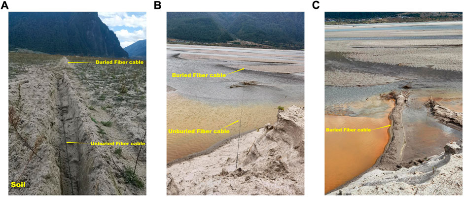
FIGURE 4. Field deployment of the optical fiber cables on land (A) and underwater across the Yigong Lake (B,C).
We select a 5-h DAS dataset in Line I and an 8-h DAS dataset in Line II for analysis, respectively. The sampling rate is 1000 Hz, and the gauge length is 10 m. The channel spacing is 1.6 m. We drop the data in the first 10 channels of Line I and the first 50 channels of Line II because of the contamination by the wandering man-walks.
Following Bensen et al. (2007), we process the DAS data with the workflow as summarized in Figure 5. The long-time raw data are split into short-time windows of 30-min long. The two ends of the segmented time series became discontinuous. We performed 10% tapering to reduce the numerical oscillation known as the Gibbs effect when filtering and performing Fourier transforms and to minimize the impact of discontinuities at both ends of the signal (Figure 6) (Xu Y et al., 2021). The influence of the DC component and linear trend is removed by de-meaning and de-trending. According to the spectrum of the original data in Figure 6, the energy is mainly concentrated below 25 Hz. We down-sample the data to 50 Hz to reduce the computational time and the memory requirements. The corresponding resampled waveform and its spectrum are shown in Figure 7. When seismic data are collected in the field, it is inevitable to be affected by environmental and human factors, resulting in a high amplitude in the time-domain signal, as shown in the red box in Figure 7.

FIGURE 5. Data processing procedure to compute NCFs in this study.
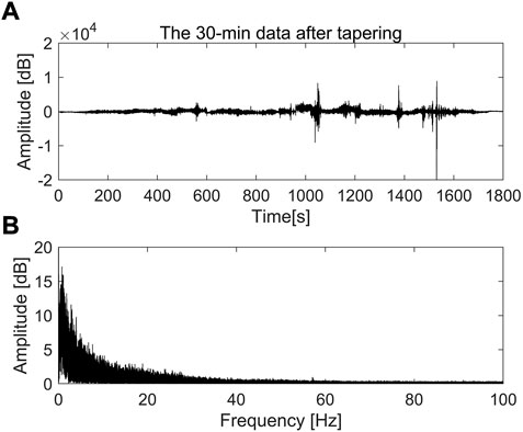
FIGURE 6. (A) Waveform, and (B) corresponding spectrum of the 30-min record of Channel 200 in Line II after tapering.
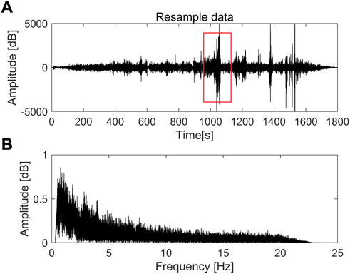
FIGURE 7. (A) Waveform, and (B) corresponding spectrum of the resampled 30-min record of Channel 200 in Line II. The red box denotes the high amplitude signal caused by environmental and human factors.
The introduction of temporal normalization can eliminate the effect of strong signals and improve the quality of the correlation results (Bensen et al., 2007). By selecting a time window of a certain length, the average of the absolute amplitude value is obtained in the time window, which is used as the weight of the center of the time window. The weight of all data is calculated by sliding the window, and then the original data is divided by the corresponding weight. Finally, the normalized sequence in the time domain is obtained. This procedure can be formulated as follows:
in which
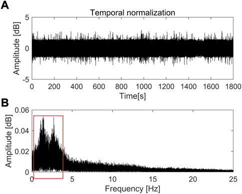
FIGURE 8. (A) Waveform, and (B) corresponding spectrum of the 30-min record of Channel 200 in Line II after temporal normalization. The red box denotes that the signal still has unbalanced high and low-frequency energy after the temporal normalization.
After the temporal normalization, the signal still has unbalanced high and low-frequency energy, and the signal spectrum is not flat, as shown in the red box in Figure 8B. Therefore, it needs to be “flattened”, also called spectrum whitening. The Hanning window
in which
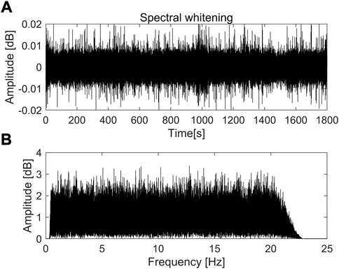
FIGURE 9. (A) Waveform, and (B) corresponding spectrum of the 30-min record of Channel 200 in Line II after spectral whitening.
Surface waves are reconstructed by using ambient noise interferometry, which has been of great interests in variant research areas (Claerbout, 1968; Weaver and Lobkis, 2001; Shapiro et al., 2005). By cross-correlating the continuous recorded ambient noise at two receiver locations, empirical Green’s functions between these two receivers can be obtained. After temporal stacking of the correlations in a long range, coherent waveforms will emerge (Campillo and Paul, 2003; Shapiro and Campillo, 2004). In the frequency domain, the cross-correlation can be formulated as:
where
After the surface wave reconstruction using ambient noise interferometry, we apply MASW (Park et al., 1999) to extract dispersion curves. First, the data in the time-offset domain are slant-stack-transformed into the frequency-velocity domain as follows:
in which
The extracted dispersion curves are further used to invert the shear wave velocity. The misfit function is defined as minimizing the difference between the picked dispersion curves and the theoretical dispersion curves calculated using the fast delta-matrix algorithm (Buchen and Ben-Hador, 1996). Considering the non-linearity and non-convexity of the inverse problem, a Mente Carlo-based global search method is used to potentially escape from being stuck at the local minimum. Detailed description of the software used in this study can be found in Olafsdottir et al. (2018) and Olafsdottir et al. (2020).
In Line I, data from Channel 11 to Channel 360 are used for calculating NCFs. From Channel 11 to Channel 185, we select every channel as a virtual source, and the other 175 channels on the right of the virtual source are cross-correlated with the virtual source. From Channel 186 to Channel 360, we select every channel as a virtual source, and the other 175 channels on the left of the virtual source are cross-correlated with the virtual source. In Line II, data from Channel 51 to Channel 350 are used for calculating NCFs. From Channel 51 to Channel 200, we select every channel as a virtual source, and the other 150 channels on the right of the virtual source are cross-correlated with the virtual source. From Channel 201 to Channel 350, we select every channel as a virtual source, and the other 150 channels on the left of the virtual source are cross-correlated with the virtual source. Next, we perform linear stacking of all the time segments for each cross-correlation pair to average the effect of temporal noise and spatial irregularity. Finally, we get 350 virtual gathers for Line I and 300 virtual gathers for Line II.
Figure 10 shows the NCFs in Line I at Channel 11 (Figure 10A) and Channel 175 (Figure 10B), and in Line II at Channel 51 (Figure 10C) and Channel 200 (Figure 10D) as virtual sources, respectively. From the reconstructed virtual gathers, it can be seen that NCFs are bilateral time functions divided into positive and negative half lags, representing positive and negative wave propagation directions, respectively. There is an obvious asymmetry that the dispersive Rayleigh-wave on the positive lag is much stronger than that on the negative lag, suggesting that the azimuth of the ambient noise is not uniformly distributed. According to the schematic layout in Figure 2, we can infer that the higher energy results from the traffic noise on the highway. Similar asymmetry is also observed by Zeng et al. (2017) from field DAS data.
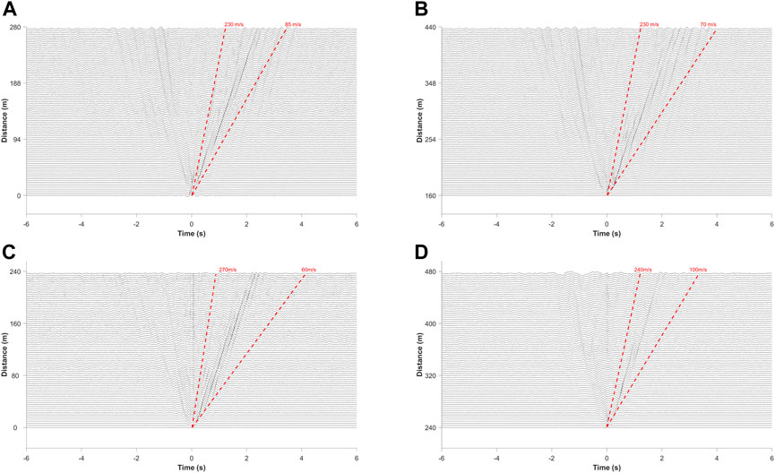
FIGURE 10. NCFs of the virtual source at Channel 11 (A), and Channel 175 (B) in Line I, and at Channel 51 (C), and Channel 200 (D) in Line II, respectively. The red dashed lines show the apparent velocity.
Before the dispersion curve extraction, the positive and negative half branches of NCFs are stacked in reverse order, and the positive half lags are reserved for subsequent processing to improve the signal-to-noise ratio (Huang et al., 2021). Such a procedure can help to mitigate the influence of uneven energy distribution of noise sources on surface wave velocity measurements.
The initial phase velocity picks are automatically chosen as the maximum value of the dispersion image in each frequency bin. Then, they are manually assigned with mode numbers and spurious picks are removed.
For the inversion of each 1D dispersion curve, we set the depth of the bottom of the interface to 90 m, and the whole model is divided into six layers. The thickness of the first layer is 8 m, the thickness of the second layer is 10 m, and the thickness of all other layers is 18 m. Since both P-wave velocity and density can affect the dispersion curve, the empirical formula of Brocher (2005) is used to convert the shear wave velocity into P-wave velocity and density. Finally, we obtain the 2D shear wave velocity profiles using cubic spline interpolation.
Figure 11 shows the dispersion images of NCFs at Channel 11 (Figure 11A) and Channel 175 (Figure 11B) in Line I, and at Channel 51 (Figure 11C) and Channel 200 (Figure 11D) in Line II, respectively. Although fundamental- and higher-mode surface waves are visible, only the fundamental mode dispersion curves, the black lines in Figure 11, are used for inversion.
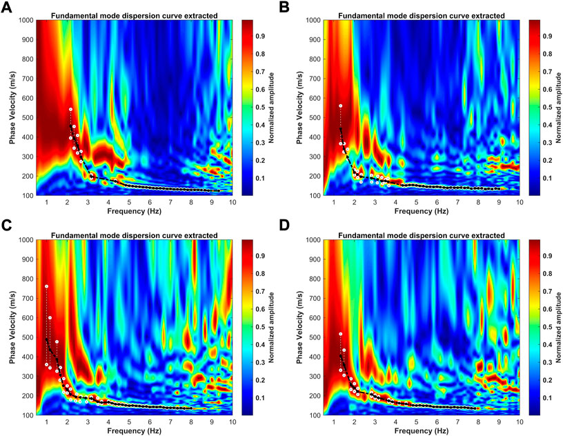
FIGURE 11. Dispersion images from the virtual gathers at Channel 11 (A) and Channel 175 (B) in Line I, and at Channel 51 (C) and Channel 200 (D) in Line II, respectively. The black curves with solid circles are the extracted fundamental model dispersion curves for inversion. The while open circles denote the upper and lower boundaries by setting as 95% of the peak value.
Figure 12 shows the 1D dispersion curve inversion results of the fundamental mode in Figure 11. The red lines denote the best inverted velocities which have the lowest misfit values. The other lines denote the top 2% best fitting models. To evaluate the accuracy of the inverted velocity models, we calculate the theoretical dispersion curves using the best inverted velocities in Figure 12. The corresponding results are shown in Figure 13 as the red lines, and they match well with the picked dispersion curves marked by the blue circles in Figure 13. Such a comparison suggests that the inverted velocity models could interpret the observed data in a good performance.
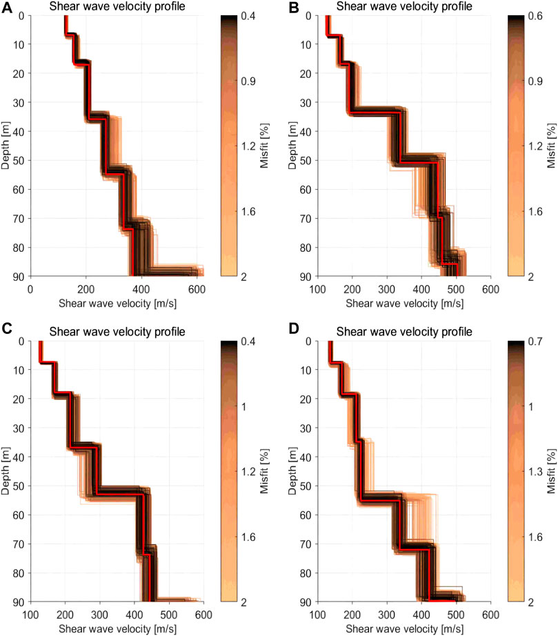
FIGURE 12. The inverted 1D shear wave velocities using the fundamental-mode dispersion curves in Figures 11A–D at Channel 11 (A) and Channel 175 (B) in Line I, and at Channel 51 (C) and Channel 200 (D) in Line II, respectively. The red lines denote the best fitted models that have the lowest misfit, and the other lines denote the top 2% best fitting models.
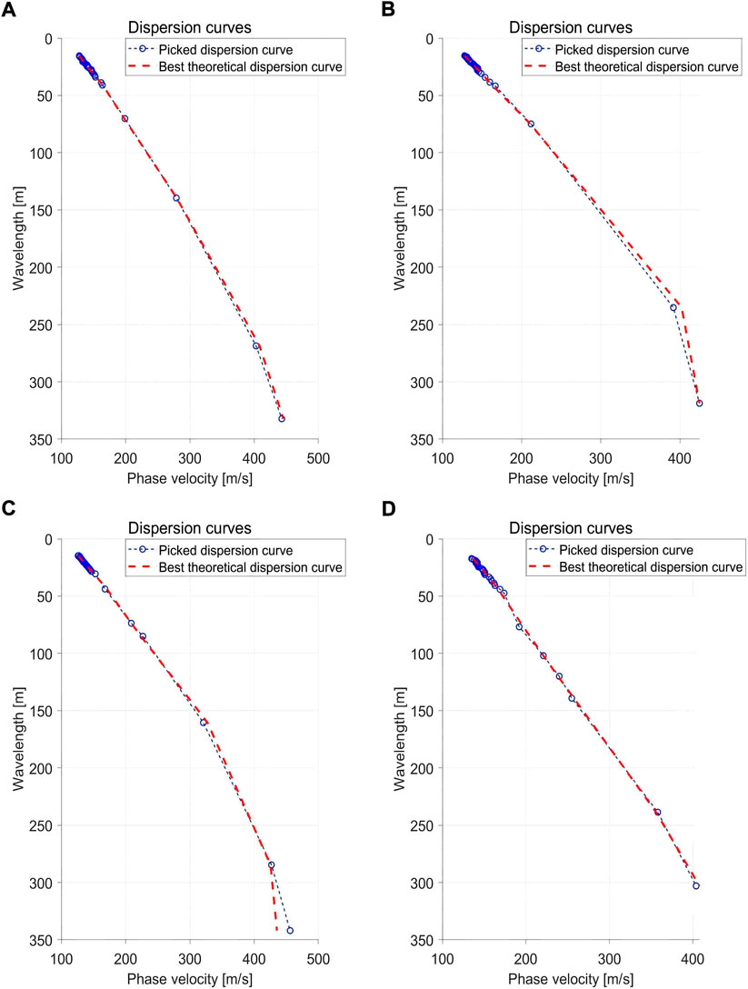
FIGURE 13. The fitting of the theoretical fundamental-mode dispersion curve using the inverted velocity in Figures 12A–D to the picked ones in Figures 11A–D at Channel 11 (A) and Channel 175 (B) in Line I, and at Channel 51 (C) and Channel 200 (D) in Line II, respectively.
The final 2D shear wave velocity profiles are shown in Figure 14. The shear wave velocity variation above 40 m depth along the two survey lines is small. There is no obvious velocity discontinuity interface, and the shear wave velocity is between 100 and 320 m/s. When the depth exceeds 40 m, the shear wave velocity gradually decreases from west to east. The lateral velocity change in Line II is greater than that in Line I. In Line I, the stratification is obvious, and the shear wave gradually decreases in the horizontal direction at the depth range of 50–70 m. In Line II, starting from the depth of 40 m, shear wave velocity presents lateral variation, and the velocity is between 250 and 350 m/s. The lateral variation of shear wave velocity increases with the gradual increase of depth, and the shear wave velocity decreases in the horizontal direction at a depth of 58–60 m.
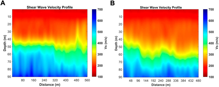
FIGURE 14. The 2D shear wave velocity profiles along the DAS Line I (A) and Line II (B).
The maximum velocity of the two profiles above the depth of 80 m is only 700 m/s, which is smaller than the velocity of the shear wave in the bedrock, so it can be inferred that the thickness of the sedimentary layer in this area should be greater than 80 m. In addition, the different features between these two profiles suggest a strong lateral variation of the sedimentary layer along the Yigong Lake. Considering the location of the lake water (blue line in Figure 2), the different shallow structures and increased thickness of the sediments in the Yigong Lake can be attributed to the accumulation of debris flow alluvium from the surrounding mountains (Zhang et al., 2021).
We have demonstrated the feasibility of using DAS to record ambient noise data in the Tibetan Plateau. By applying the well-established seismic interferometry to the DAS data, we can reveal the shallow sedimentary structure of the Yigong Lake, which is very helpful to understand the dynamic evolution of this area. Considering the extreme conditions of the Tibetan Plateau, it is difficult, if not possible, to deploy traditional geophones or portable nodes for environmental seismology study, our method can be a promising alternative for the interested readers.
We should note that since the surface wave inversion is highly non-unique, further studies are needed to verify the reliability of the inversion results by incorporating other geological information, such as the drilling data. Due to the limited recording time, we could not get enough low frequency information below 1 Hz. Only when these low frequency data are available, we can get access to the deeper parts to reveal the actual depth of the bedrock. In addition, we only use the land data and a small portion of the underwater data of Line I in this study. The noise characteristics in the rest parts are more complex than those used in this study, which need further processing and evaluation. Future work with integration of the complete DAS dataset might give chances for a better interpretation of the geologic evolution history of the Yigong Lake.
This study introduces a shallow sedimentary structure imaging method in extreme conditions of the Yigong Lake in the Tibetan Plateau using ambient noise data recorded by DAS. By applying proper data pre-processing and seismic interferometry to the ambient noise data, clear NCFs are obtained and surface waves can be easily identified. Dispersion curves are then extracted using MASW and are inverted to get the shear wave velocity model of the study area. The results show that the lateral variation is not evident in the shallow subsurface layer, and the lateral inhomogeneity of shear wave velocity increases with depth. Since the shear wave velocity is smaller than conventional bedrock at depths greater than 80 m, it can be assumed that the sedimentary thickness is greater than 80 m in the Yigong Lake area. The increased thickness is likely due to debris-flow deposits in the surrounding mountains. The low-cost, high-density acquisition and processing of DAS data demonstrate the effectiveness and practicality of DAS in detecting shallow sedimentary structures in extreme environments in the Tibetan Plateau. We are expecting that DAS will be a powerful tool for studies of remote and harsh environments in the future.
The datasets presented in this article are not readily available because it is still being used for scientific research. Requests to access the datasets should be directed to the corresponding author.
JY, JZ, and JG studied the method, processed the data and wrote the draft of the manuscript. JY, HZ, and DD acquired the DAS data in the field. HZ planned the project, and TX designed the DAS system. All the authors contributed to the final manuscript.
This research was financially supported by the Second Tibetan Plateau Scientific Expedition and Research Program (Grant No. 2019QZKK0708), the National Natural Science Foundation of China (Grant Nos. 42004096, 41974109, and 61875184), Shanghai Sheshan National Geophysical Observatory (No. SSOP202205), the Fundamental Research Funds for the Central Universities of China, the Scientific Instrument Developing Project of the Chinese Academy of Sciences (Grant No. YJKYYQ20190075), the Strategic Priority Research Program of the Chinese Academy of Sciences (Grant Nos. XDA20070301 and XDA22040105), the Grants of the Wong K.C. Education Foundation (No. GJTD-201904), and the Research Program of Sanya Yazhou Bay Science and Technology City (Grant No. SKJC-2020-01-009).
The authors declare that the research was conducted in the absence of any commercial or financial relationships that could be construed as a potential conflict of interest.
All claims expressed in this article are solely those of the authors and do not necessarily represent those of their affiliated organizations, or those of the publisher, the editors and the reviewers. Any product that may be evaluated in this article, or claim that may be made by its manufacturer, is not guaranteed or endorsed by the publisher.
Bensen, G. D., Ritzwoller, M. H., Barmin, M. P., Levshin, A. L., Lin, F. F., Moschetti, M. P., et al. (2007). Processing seismic ambient noise data to obtain reliable broad-band surface wave dispersion measurements. Geophys. J. Int. 169, 1239–1260. doi:10.1111/j.1365-246X.2007.03374.x
Booth, A. D., Christoffersen, P., Schoonman, C., Clarke, A., Hubbard, B., Law, R., et al. (2020). Distributed acoustic sensing of seismic properties in a borehole drilled on a fast-flowing Greenlandic outlet glacier. Geophys. Res. Lett. 47, e2020GL088148. doi:10.1029/2020GL088148
Brocher, T. M. (2005). Empirical relations between elastic wavespeeds and density in the Earth's crust. Bull. Seismol. Soc. Am. 95 (6), 2081–2092. doi:10.1785/0120050077
Campillo, M., and Paul, A. (2003). Long-range correlations in the diffuse seismic coda. Science 299, 547–549. doi:10.1126/science.1078551
Claerbout, J. F. (1968). Synthesis of a layered medium from its acoustic transmission response. Geophysics 33, 264–269. doi:10.1190/1.1439927
Daley, T. M., Miller, D. E., Dodds, K., Cook, P., and Freifeld, B. M. (2016). Field testing of modular borehole monitoring with simultaneous distributed acoustic sensing and geophone vertical seismic profiles at Citronelle, Alabama. Geophys. Prospect. 64 (5), 1318–1334. doi:10.1111/1365-2478.12324
Dou, S., Lindsey, N., Wagner, A. M., Daley, T. M., Freifeld, B., Robertson, M., et al. (2017). Distributed acoustic sensing for seismic monitoring of the near surface: A traffic-noise interferometry case study. Sci. Rep. 7, 11620. doi:10.1038/s41598-017-11986-4
Fang, G., Li, Y. E., Zhao, Y., and Martin, E. R. (2020). Urban near-surface seismic monitoring using distributed acoustic sensing. Geophys. Res. Lett. 47 (6), e2019GL086115. doi:10.1029/2019GL086115
Guo, C., Montgomery, D. R., Zhang, Y., Zhong, N., Fan, C., Wu, R., et al. (2020). Evidence for repeated failure of the giant Yigong landslide on the edge of the Tibetan Plateau. Sci. Rep. 10, 14371. doi:10.1038/s41598-020-71335-w
Hartog, A. H. (2017). An introduction to distributed optical fibre sensors. Florida, United States: CRC Press.
Huang, X., Ding, Z. F., Ning, J. Y., and Chang, L. J. (2021). Rayleigh wave phase velocity and azimuthal anisotropy of central North China Craton derived from ambient noise tomography. Chin. J. Geophys. 64, 2701–2715. doi:10.6038/cjg2021O0442
Jousset, P., Reinsch, T., Ryberg, T., Blanck, H., Clarke, A., Aghayev, R., et al. (2018). Dynamic strain determination using fibre-optic cables allows imaging of seismological and structural features. Nat. Commun. 9, 2509. doi:10.1038/s41467-018-04860-y
Karplus, M., and Schmandt, B. (2018). Preface to the focus section on geophone array seismology. Seismol. Res. Lett. 89 (5), 1597–1600. doi:10.1785/0220180212
Klaasen, S., Paitz, P., Lindner, N., Dettmer, J., and Fichtner, A. (2021). Distributed acoustic sensing in volcano-glacial environments-Mount Meager, British Columbia. JGR. Solid Earth 126, e2021JB022358. doi:10.1029/2021JB022358
Kohler, M. D., Hafner, K., Park, J., Irving, J. C., Caplan-Auerbach, J., Collins, J., et al. (2020). A plan for a long-term, automated, broadband seismic monitoring network on the global seafloor. Seismol. Res. Lett. 91, 1343–1355. doi:10.1785/0220190123
Lellouch, A., and Biondi, B. L. (2021). Seismic applications of downhole DAS. Sensors 21 (9), 2897. doi:10.3390/s21092897
Lindsey, N. J., Dawe, T. C., and Ajo-Franklin, J. B. (2019). Illuminating seafloor faults and ocean dynamics with dark fiber distributed acoustic sensing. Science 366, 1103–1107. doi:10.1126/science.aay5881
Lindsey, N. J., Martin, E. R., Dreger, D. S., Freifeld, B., Cole, S., James, S. R., et al. (2017). Fiber-optic network observations of earthquake wavefields. Geophys. Res. Lett. 44 (23), 11–792. doi:10.1002/2017GL075722
Lindsey, N. J., and Martin, E. R. (2021). Fiber-optic seismology. Annu. Rev. Earth Planet. Sci. 49, 309–336. doi:10.1146/annurev-earth-072420-065213
Mateeva, A., Lopez, J., Potters, H., Mestayer, J., Cox, B., Kiyashchenko, D., et al. (2014). Distributed acoustic sensing for reservoir monitoring with vertical seismic profiling. Geophys. Prospect. 62, 679–692. doi:10.1111/1365-2478.12116
Nishikawa, T., Matsuzawa, T., Ohta, K., Uchida, N., Nishimura, T., and Ide, S. (2019). The slow earthquake spectrum in the Japan Trench illuminated by the S-net seafloor observatories. Science 365, 808–813. doi:10.1126/science.aax5618
Nishimura, T., Emoto, K., Nakahara, H., Miura, S., Yamamoto, M., Sugimura, S., et al. (2021). Source location of volcanic earthquakes and subsurface characterization using fiber-optic cable and distributed acoustic sensing system. Sci. Rep. 11, 6319. doi:10.1038/s41598-021-85621-8
Olafsdottir, E. A., Erlingsson, S., and Bessason, B. (2020). Open-source MASW inversion tool aimed at shear wave velocity profiling for soil site explorations. Geosciences 10 (8), 322. doi:10.3390/geosciences10080322
Olafsdottir, E. A., Erlingsson, S., and Bessason, B. (2018). Tool for analysis of multichannel analysis of surface waves (MASW) field data and evaluation of shear wave velocity profiles of soils. Can. Geotech. J. 55, 217–233. doi:10.1139/cgj-2016-0302
Park, C. B., Miller, R. D., and Xia, J. H. (1999). Multichannel analysis of surface waves. Geophysics 64, 800–808. doi:10.1190/1.1444590
Parker, T., Shatalin, S., and Farhadiroushan, M. (2014). Distributed Acoustic Sensing–a new tool for seismic applications. First Break 32 (2), 61–69. doi:10.3997/1365-2397.2013034
Shang, Y., Yang, Z., Li, L., Liao, Q., and Wang, Y. (2003). A super-large landslide in Tibet in 2000: Background, occurrence, disaster, and origin. Geomorphology 54, 225–243. doi:10.1016/S0169-555X(02)00358-6
Shao, J., Wang, Y., Zheng, Y., Yao, Y., Wu, S., Yang, Z., et al. (2022). Near-surface characterization using urban traffic noise recorded by fiber-optic distributed acoustic sensing. Front. Earth Sci. (Lausanne). 10, 943424. doi:10.3389/feart.2022.943424
Shapiro, N. M., and Campillo, M. (2004). Emergence of broadband Rayleigh waves from correlations of the ambient seismic noise. Geophys. Res. Lett. 31, L07614. doi:10.1029/2004GL019491
Shapiro, N. M., Campillo, M., Stehly, L., and Ritzwoller, M. H. (2005). High-resolution surface-wave tomography from ambient seismic noise. Science 307, 1615–1618. doi:10.1126/science.1108339
Shinohara, M., Yamada, T., Akuhara, T., Mochizuki, K., and Sakai, S. I. (2022). Performance of seismic observation by distributed acoustic sensing technology using a seafloor cable off Sanriku, Japan. Front. Mar. Sci. 9, 844506. doi:10.3389/fmars.2022.844506
Sladen, A., Rivet, D., Ampuero, J. P., De Barros, L., Hello, Y., Calbris, G., et al. (2019). Distributed sensing of earthquakes and ocean-solid Earth interactions on seafloor telecom cables. Nat. Commun. 10, 5777. doi:10.1038/s41467-019-13793-z
Spica, Z. J., Perton, M., Martin, E. R., Beroza, G. C., and Biondi, B. (2020). Urban seismic site characterization by fiber-optic seismology. J. Geophys. Res. Solid Earth 125 (3), e2019JB018656. doi:10.1029/2019JB018656
Walter, F., Gräff, D., Lindner, F., Paitz, P., Köpfli, M., Chmiel, M., et al. (2020). Distributed acoustic sensing of microseismic sources and wave propagation in glaciated terrain. Nat. Commun. 11, 2436. doi:10.1038/s41467-020-15824-6
Wang, H. F., Zeng, X., Miller, D. E., Fratta, D., Feigl, K. L., Thurber, C. H., et al. (2018). Ground motion response to an ML 4.3 earthquake using co-located distributed acoustic sensing and seismometer arrays. Geophys. J. Int. 213 (3), 2020–2036. doi:10.1093/gji/ggy102
Weaver, R. L., and Lobkis, O. I. (2001). Ultrasonics without a source: Thermal fluctuation correlations at MHz frequencies. Phys. Rev. Lett. 87 (13), 134301. doi:10.1103/PhysRevLett.87.134301
Williams, E. F., Fernández-Ruiz, M. R., Magalhaes, R., Vanthillo, R., Zhan, Z., González-Herráez, M., et al. (2019). Distributed sensing of microseisms and teleseisms with submarine dark fibers. Nat. Commun. 10, 5778. doi:10.1038/s41467-019-13262-7
Xu, T., Feng, S., Li, F., Ma, L., and Yang, K. (2021). “Distributed acoustic sensing system based on phase-generated carrier demodulation algorithm,” in Distributed Acoustic Sensing in Geophysics, Editor Y. Li, M. Karrenbach, and J. B. Ajo-Franklin. doi:10.1002/9781119521808.ch4
Xu, Y., Lebedev, S., Meier, T., Bonadio, R., and Bean, C. J. (2021). Optimized workflows for high-frequency seismic interferometry using dense arrays. Geophys. J. Int. 227, 875–897. doi:10.1093/gji/ggab260
Yu, C., Zhan, Z., Lindsey, N. J., Ajo-Franklin, J. B., and Robertson, M. (2019). The potential of DAS in teleseismic studies: Insights from the Goldstone experiment. Geophys. Res. Lett. 46 (3), 1320–1328. doi:10.1029/2018GL081195
Zeng, X., Lancelle, C., Thurber, C., Fratta, D., Wang, H., Lord, N., et al. (2017). Properties of noise cross-correlation functions obtained from a distributed acoustic sensing array at Garner Valley, California. Bull. Seismol. Soc. Am. 107 (2), 603–610. doi:10.1785/0120160168
Zhang, H., Xu, T. W., Pei, S. P., and Zhao, J. M. (2021). Application of distributed acoustic sensing in structural investigation of Lake Yigong in Tibet. Earth Sci. Front. 28, 227–234. doi:10.13745/j.esf.sf.2021.11.10
Zhou, J. W., Cui, P., and Hao, M. H. (2016). Comprehensive analyses of the initiation and entrainment processes of the 2000 Yigong catastrophic landslide in Tibet, China. Landslides 13, 39–54. doi:10.1007/s10346-014-0553-2
Keywords: distributed acoustic sensing, sedimentary thickness, Tibetan Plateau, ambient noise tomography, seismic interferometry
Citation: Yang J, Zhou J, Zhang H, Xu T, Deng D and Geng J (2023) Revealing the shallow soil structure of the Yigong Lake in the Tibetan Plateau using a portable distributed acoustic sensing interrogator. Front. Earth Sci. 10:1018116. doi: 10.3389/feart.2022.1018116
Received: 12 August 2022; Accepted: 17 October 2022;
Published: 11 January 2023.
Edited by:
Xiaowei Chen, University of Oklahoma, United StatesReviewed by:
Xiaoyun Wan, China University of Geosciences, ChinaCopyright © 2023 Yang, Zhou, Zhang, Xu, Deng and Geng. This is an open-access article distributed under the terms of the Creative Commons Attribution License (CC BY). The use, distribution or reproduction in other forums is permitted, provided the original author(s) and the copyright owner(s) are credited and that the original publication in this journal is cited, in accordance with accepted academic practice. No use, distribution or reproduction is permitted which does not comply with these terms.
*Correspondence: Heng Zhang, emhhbmdoZW5nNDE1QGl0cGNhcy5hYy5jbg==
Disclaimer: All claims expressed in this article are solely those of the authors and do not necessarily represent those of their affiliated organizations, or those of the publisher, the editors and the reviewers. Any product that may be evaluated in this article or claim that may be made by its manufacturer is not guaranteed or endorsed by the publisher.
Research integrity at Frontiers
Learn more about the work of our research integrity team to safeguard the quality of each article we publish.