 Xuewei Liu1,2*Dongping Li1Yunpeng Jia1Yang Liyong1Gou Xiaoting1Zhao Tao1Chen Ziwei1Li Mao1Wang Juan1Sui Xiangyun1Zhao Donghua1Tang Hongxia1Li Yulin2*Zhang Yu2
- 1Petroleum Engineering Research Institute, PetroChina Dagang Oilfield Company, Tianjin, China
- 2State Key Laboratory of Oil and Gas Reservoir Geology and Exploitation, Southwest Petroleum University, Chengdu, China
Shale oil is mainly extracted by fracturing. However, it is difficult to determine the optimum construction parameters to obtain maximum productivity. In this paper, a fuzzy comprehensive production evaluation model for fractured shale oil horizontal wells based on random forest algorithm and coordinated principal component analysis is proposed. The fracturing parameters of the target wells are optimized by combining this model with an orthogonal experimental design. The random forest algorithm was used to calculate the importance of data sample factors. The main controlling factors of the production of fractured horizontal wells in shale oil were obtained. To reduce the noise of the sample data, principal component analysis was used to reduce the dimensions of the main control factors. Furthermore, the random forest algorithm was used to determine the weight of the principal components after reducing the dimensionality. The membership function of the main control factors after reducing dimensionality was established by combining the fuzzy statistics and assignment methods. In addition, the membership matrix of the effect prediction of fractured horizontal wells in shale oil was determined. The fuzzy comprehensive evaluation method is used to score and evaluate the effect of fractured horizontal wells. Combined with the orthogonal experimental design method, the optimized parameter design of a fractured horizontal well considering the comprehensive action of multiple parameters is realized. After construction according to the optimized parameters, production following fracturing increases significantly. This verifies the rationality of the optimization method that is proposed in this paper.
1 Introduction
Shale oil resources are rich, and show good exploration and development potential (Rodriguez and Soeder, 2015). Shale oil reservoirs have strong heterogeneity, small pore throat structure, complex fluid phase, and oil and gas properties. The success of exploration and development is due to the effective “liberation” of the reservoir by multi-cluster volume fracturing of horizontal wells (Hu et al., 2020). Meanwhile, the hydraulic fracturing effect of shale oil mainly depends on the matching of construction parameters and geological parameters. The fracturing optimization design largely determines the fracturing improvement effect. The productivity of fractured horizontal wells for shale oil can be improved by establishing an effective optimization method for the construction parameters of fractured horizontal wells for shale oil (Rahmanifard and Plaksina, 2018).
Currently, there are two main methods for fracturing parameters optimization. First, a fracture propagation model is established to simulate the fracture extension process in the fracturing process. The fracture parameters are optimized by maximizing the reconstruction volume (Guo et al., 2015). However, the actual fracture extension is very complex, and the simplified simulation model cannot accurately reflect the real situation of reservoir fracture extension. Second, the reservoir numerical simulation method has been used to set the cumulative production or stimulation period as the objective function, and the optimal objective function has been used to select the best fracture parameters (Moradidowlatabad and Jamiolahmady, 2018). However, it is easy to form a multi-scale fracture network with a highly complex topological structure in the large-scale hydraulic fracturing of shale oil. In addition, the non-Darcy seepage of shale nanopores lengthens the time required for the numerical simulation of a shale reservoir, which greatly reduces the efficiency of the parameter optimization (Xiao et al., 2022). The optimization of the construction parameters of fractured horizontal wells in shale oil faces considerable challenges thanks to the complexity of the shale reservoir’s characteristics and fracture system, as well as the large number of design variables (Ma et al., 2022).
A large amount of valuable fracturing operation and production performance data have been gathered. Consequently, data mining and machine learning are increasingly being used in the study of fracturing parameter optimization. For the supervised machine-learning model with small samples, the approximate model of objective function and constraint function with variable variation is constructed from a small number of sample points. For wells that need to optimize fracturing parameters, the stimulation effect of fractured wells under different parameter combinations is calculated by changing the combination of fracturing parameters and using the established approximate model to optimize the fracturing parameters. Deng et al. (2022) proposed a new integrated optimization algorithm that is based on the field data, aiming at NPV, and realized the integrated optimization of continuous and discrete fracture parameters. Based on a large number of CFD modeling results, Wang et al. (2022a) established an artificial neural network model to optimize construction parameters, which can then be used to optimize the design of the perforation and fracturing parameters. Li-Yang et al. (2022) adopted a BP neural network and genetic algorithm to establish a productivity prediction model and form a genetic optimization design method for horizontal well fracturing. Zhang et al. (2021) used the unsupervised K-means clustering algorithm based on Euclidean distance to cluster reservoirs according to reservoir seepage and geo-mechanical parameters, identify the compressible area of the reservoir fracturing stage, and obtain the fracturing area and fracture morphology through numerical simulation of the reservoir perforation and fracturing process to evaluate the fracturing effect. However, these studies only proposed the optimization of some construction parameters, which should also include horizontal stage length, number of fracturing stages, proppant consumption, and fluid volume (Wang and Chen, 2019). Based on this, some scholars have further established the optimal design model by considering the matching of construction parameters and geological parameters.
Shahkarami et al. (2018) used a publicly available data database from more than 2000 Wells in southwest Pennsylvania to establish a hydraulic fracturing parameter optimization design model that is based on linear regression, support vector machine, artificial neural network, Gaussian process, and other machine-learning methods. Through sensitivity analysis, Nguyen-Le and Shin (2019) determined the framework of controlling factors to put forward a dynamic economic index, and realized the Np value optimization model considering the comprehensive influence of reservoir parameters and fracturing parameters. Duplyakov et al. (2020) used a boosting algorithm to optimize hydraulic fracturing design based on the data of 22 oil fields, which considered the influence of geological parameters on the optimization of construction parameters. Tan et al. (2021) took the statistical data of fractured wells in WY block as the data set and established a production prediction model based on six machine-learning algorithms, including random forest, support vector regression, back propagation neural network, XGBoost, LightGBM, and multiple linear regression. They then optimized each construction parameter with the goal of improving yield and the cost-profit ratio. Guo et al. (2022) adopted the PCA-GRA method to determine the main control factors of tight oil production. They established a BP neural network model with tight oil production as output and main control factors as input. This model could predict production and optimize construction parameters. Taking 75 fractured horizontal wells in Mahu area as an example, Ma et al. (2021) adopted the random forest algorithm to determine the main control factors of post-pressure productivity according to 16 influencing factors in two types of reservoirs and engineering. They established a productivity prediction model that is optimized by a genetic algorithm with inverse propagation algorithm and neural network, and then optimized the fracturing design of horizontal wells based on this. Hui et al. (2021) used Pearson correlation coefficient and feature selection process method. They used 13 geological and construction parameters (e.g., logging and core experiment) as input variables, and established an optimization model with the goal of maximizing accumulations in 12 months through the Extra Trees algorithm. Their results showed that a 73% increase in fluid volume and a 38% increase in proppant use could double post-fracture production. Under boundary constraints, Duplyakov et al. (2022) used the high-dimensional black box approximation function to optimize fracturing design parameters based on Ridge regression and CatBoost algorithm. They also used particle swarm optimization, sequential least squares programming, surrogate optimization model and differential evolution optimization method to solve the problem. Xiao et al. (2022) proposed a machine-learning assisted global optimization framework that is based on radial basis functions, K-nearest neighbors, and multi-layer perceptrons to quickly obtain the optimal fracture parameters. Syed et al. (2022) established Pearson correlation estimation between each pair of input parameters and developed a prediction model using deep learning that could integrate basic geological information with a completion strategy. Wang et al. (2022b) used fracturing fluid (e.g., reflux ratio and first production) as the objective function, based on the least square method, support vector regression algorithm, and the non-dominant sorting genetic algorithm. They established a fracturing parameters optimization design method using length, horizontal well fracturing series, fracture length, fracture fluid injection, the viscosity of fracturing fluid, fracturing fluid volume, and amount of proppant as optimization variables. They were then able to establish the optimization framework of objective parameters.
This optimization design method of fracturing parameters has achieved satisfactory results. However, the fracturing parameter optimization method based on machine learning still experiences the following problems. First, the reservoir parameter values are derived from the limit value and the average deterministic numerical, without fully considering the reservoir parameters, due to uncertainties or under experimental apparatus, experimental method, or calculation error (e.g., ignoring that these parameters have a characteristic certain fuzziness). Second, when the reservoir parameters, fracturing parameters, and stimulation effect of fractured wells are used to establish a mathematical relationship through mathematical statistics, there is always a strong correlation between these influencing factors. When establishing the optimization model of fracturing parameters, a large number of parameters are directly input into the model. However, the network structure constructed is too complex and the learning of the network model is difficult. The deviation of optimal fracturing parameters will increase when there is no definite mathematical relationship between the stimulation effect and reservoir parameters, and between the fracturing parameters and reservoir parameters. Finally, there are too few optimal fracturing parameters to choose and the final optimization may only be equivalent to finding the local optimal fracturing parameters rather than the global optimal fracturing parameters in the true sense.
To tackle the issues of optimizing the shale oil construction parameters, random forest was used to determine the main control factors and weights of the fracturing effect. The dimensionality of the parameters affecting the fracturing effect was reduced by principal component analysis. The principal components after reducing dimensionality were used as the input parameters of the fuzzy comprehensive evaluation model. The fuzzy mathematical evaluation method was introduced to establish the fracturing effect evaluation model considering the comprehensive effects of single factor and multiple factors, predict the stimulation effect of different fracturing construction parameters, and to select the optimal scheme.
2 Data sources and research methods
2.1 Study area overview
The research area is located between Cangxian Uplift, Xuhei Uplift, and Kongdian Uplift in the hinterland of the Bohai Bay Basin. It is a fault-depression lake basin that was developed under the background of Paleogene regional stretching, and is divided into five tectonic units: Nanpi slope, Kongdong slope, Kongxi slope, Kongdian tectonic belt, and Shenusi faulting (Ren et al., 2010). The main sedimentary strata in the lake basin are Kongdian Formation, which are Kong3 member, Kong2 member, and Kong1 member (from bottom to top). Among them, Kong2 member is a lake flood deposition of Kongdian Formation with thick mud shale and sandstone, coarse-grained deposition of braided river delta medium fine sandstone is developed at the edge of the lake basin, and mud shale is mainly found in the middle of the lake basin. The second member of the hole can be divided into four fourth-order sequences (SQEk24—SQEk21) and 10 fifth-order sequences (Ek21SQ①—Ek24SQ⑩) from bottom to top (Pu et al., 2015), among which SQEk23—SQEk21 is a shale segment with high organic matter abundance 300–500 m thick, covering an area of 1187 km2. The 21 layers which can be traced and compared in the whole region, which were further divided. The preliminary exploration practice shows that, first, the reservoir has strong heterogeneity, complex physical properties, and many lithologic types encountered in a single well. Post-pressure oil production is comprehensively affected by geological factors, engineering parameters and production system, and the fracturing effect is quite different. It is therefore necessary to further clarify the main controlling factors that affect the fracturing effect. Second, the production of different wells varies greatly after fracturing, which reflects the poor matching between the construction parameters of some wells and the reservoir, which affects the stimulation effect. Consequently, research on the optimization of construction parameters matching the geological characteristics of single well is urgently required.
2.2 Data source and analysis
In total, 24 fractured horizontal wells of shale oil in area W were taken as samples to fully collect on-site geological, engineering, and production parameters, as well as production data. The collected data results are shown in Table 1. Well W24 was selected as the test well to verify the rationality of the proposed method and to optimize the construction parameters. The remaining fractured wells were used as training wells to obtain the main control factors of the production of shale oil fractured horizontal wells. The function model of fuzzy comprehensive score and production was fitted.
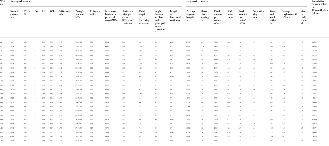
TABLE 1. W Data collection results.
2.2.1 Main control factors and weight determination method selection
The characteristics of tight shale oil reservoirs and low-pressure coefficient in W area determine whether industrial production can only be obtained through large-scale reconstruction, and whether the oil production is affected by geological and engineering factors. To establish an optimization method for the construction parameters of fractured horizontal wells, the construction parameters can quickly and efficiently be optimized by identifying the main controlling factors and assigning reasonable weights.
In this paper, the random forest algorithm is chosen to select representative main control factors. Compared with traditional prediction models, random forest has the following advantages. First, it has strong adaptability to data sets, does not need the data to meet the preset assumptions or specific functional forms, is insensitive to multivariate collinearity, and is robust to missing data and unbalanced data. Second, the modeling is simple and efficient, and the generalization ability is strong, which can quickly capture the inflection point by using the advantages of multi-path parallel decision tree. With the increase of the number of regression trees, the error of random forest model can be reduced on the whole. Compared with a support vector machine or an artificial neural network, it has fewer calibration parameters, and only needs to specify the number of regression trees and the number of features sampled from each bifurcation node, consequently the training process is simpler and faster. Third, it can deal with high-dimensional data sets and random forest can avoid the common problems of machine learning (e.g., over-fitting and under-fitting). Finally, random forest can get the weight of each variable and avoid the interference of subjective factors when the weight is artificially assigned. Therefore, this paper intends to use random forest to analyze the main control factors and determine the weight.
2.2.2 Principle of the random forest algorithm
The random forest algorithm is another combination prediction algorithm that was proposed by Breiman after the Bagging algorithm (Breiman, 2001). Based on decision trees, it builds multiple decision trees through random repeated sampling technology (Boostrap technology; Freeman, 1998) and random node splitting technology, and finally combines the prediction results of a large number of decision trees and outputs them as a whole. Ensemble learning through multiple decision trees can effectively overcome the problems of over-fitting and low classification accuracy of a single decision tree, and can effectively reduce the generalization error of the learning system (He et al., 2020). The steps that are used by the random forest method to determine the weight are described in the following subsections.
2.2.2.1 Screening the main control factors
The data that are randomly sampled and not drawn during random forest modeling are called out-of-pocket data sets, which are not involved in the fitting of the training set model and can be used to test the generalization ability of the model (Lei et al., 2020). When ranking the importance of the model, the corresponding out-of-pocket data is used to calculate its out-of-pocket error r1. The order of a feature in the out-of-pocket data is then randomly transformed and the out-of-pocket error r2 is calculated again. Assuming that the random forest has N trees, the importance of a feature I is:
where I is the importance of a feature, and is dimensionless; N is the number of trees in the random forest, and is dimensionless; r1 is the out-of-pocket error, and is dimensionless; and r2 is the out-of-pocket error of a feature sequence after random transformation, and is dimensionless.
The importance of each characteristic parameter of 23 trained fractured horizontal wells can be obtained using the random forest algorithm, among which the most important is the main control factor of the production of fractured horizontal wells in shale oil. The screened results according to the above principles are shown in Table 2. As can be seen from Table 2, the rock brittleness index and the sand-liquid ratio in the main control factors of the production of fractured horizontal wells in shale oil in this block are significantly more important than other main control factors in geological parameters, which indicates that these main control factors contribute greatly to the production of fractured horizontal wells in shale oil.
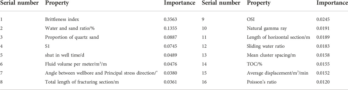
TABLE 2. Screening results of the main control factors.
2.2.2.2 Weight determination
With regard to random forests, impurity has been adopted as the best division of the measurement classification tree and the impurity calculation has been made with the Gini index method, which is one of the most widely used segmentation rules. Assuming that the set T contains records of k categories, then the Gini index is:
where Gini(T) is the Gini index of set T, and is dimensionless; k is the number of categories, and is dimensionless; and pj denotes the frequency of T occurrence of category j, and is dimensionless.
The maximum useful information can be obtained when the Gini(T) minimum is 0 (i.e., all of the records on this node belong to the same category). Gini(T) is maximum when all of the records in this node are uniformly distributed with respect to the category field, which indicates that the minimum useful information is obtained. If the set T is divided into s parts Ti (i = 1,2...,s). To calculate the Gini coefficient, the reduction in the Gini coefficient of the variable xi used to split at each split node is calculated. Then, the Gini index for this segmentation is:
where Ginisplit(T) is the segmented Gini index, and is dimensionless.
For the classification regression tree, if the node T does not satisfy that the samples in T belong to the same category or there is only one sample left in T, then this node is a non-leaf node. The original segmentation Gini index of the ith classification regression tree is Ginisplit (xi), and the Gini index after randomly replacing the variable attribute value j of the separation point is Ginisplit (xij). Therefore, the importance of attribute j in the corresponding single classification regression tree can be expressed as Ginisplit (xi)-Ginisplit(xij). The importance
where
The weight of indicator variables is:
where wj is the weight coefficient of the jth index variable, and is dimensionless; and n is the number of indicator attributes, and is dimensionless.
Because the dimensionality of the main control factors needs to be reduced before the weight is determined, the weight results of each principal component are shown in Section 3.1 (Model Establishment).
2.3 Optimization of fracturing parameters
2.3.1 Reducing dimensionality with principal component analysis
The random forest algorithm requires high levels of time and cost, and is only suitable for small data sets (Chen and Min, 2022). Taking the main control factors of the production of a large number of shale oil fractured horizontal wells as input parameters of the model will increase the difficulty and complexity of the analysis problem, and reduce the optimization efficiency. The problem can be simplified based on the principal component analysis of the dimensionality reduction, integrating multiple correlation factors for the linear unrelated principal component, using the correlation between the main control factors with a dimension reduction after less principal components instead of many factors, and using the principal component as much as possible to leave the factors reflected in information. The calculation steps are as follows:
1) Data collection, with m evaluation fracturing wells and e main control factor indicators, a sample matrix a with size of m×e can be formed:
where a is the sample matrix; aij is the main control factor; and aj is the vector of main control factors.
2) When the index dimensions are inconsistent, the mean and standard deviation are calculated to obtain standardized data (Li et al., 2020), and the correlation coefficient matrix R is established. The original sample matrix is normalized to:
where A is the sample matrix after standardization; Aij is the main control factor after standardization; and Aj is the normalized vector of master factors.
Thus, the corresponding correlation coefficient matrix of the sample matrix can be obtained:
where R is the correlation coefficient matrix; and rij is the correlation coefficient, where:
The correlation coefficient matrix shows the correlation degree among e indexes.
3) Calculate the eigenvalues and eigenvectors of R.
Eigenvalues:
Feature vector:
4) Calculate the variance contribution rate bi and cumulative contribution rate b(o) of each eigenvector of corresponding eigenvalue:
where bi is the variance contribution rate of each eigenvector of the eigenvalue, and is dimensionless; and b(o) is the cumulative contribution rate of each eigenvector of the eigenvalue, and is dimensionless.
5) Calculate the number of principal components and calculate the expression of each principal component. In general, the number of eigenvectors corresponding to eigenvalues whose value is greater than or equal to 1 and cumulative contribution rate exceeds 85% is taken as the number of principal components. The score of each principal component is calculated according to the linear expression composed of its corresponding feature vector and each index. The ith principal component Fi is calculated as follows:
where Fi is the ith principal component, and is dimensionless.
The data of 16 main control factors selected from the collected data of 23 fractured horizontal wells were used as input, and the output was used as the objective function to reduce the dimension of principal components. The variance contribution rate of principal components is shown in Figure 1. The analysis found that the information of the first six principal components accounted for 87% in total, so the first six principal components were selected to replace the original 16 feature parameters.
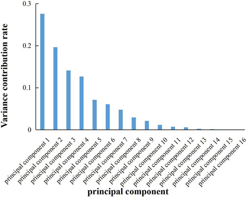
FIGURE 1. Variance explained by principal components.
The characteristics of principal components corresponding to the factors of the six principal components are shown in Table 3. According to the data in Table 3, the main control factor data selected from different fractured horizontal wells are substituted into Eqs 7, 14 to obtain the principal component values of different fractured wells. The results are shown in Supplementary Table S1. The normalized principal component matrix is obtained as shown in Supplementary Table S2.

TABLE 3. Characteristics of the principal components corresponding to the main control factors.
2.3.2 Fuzzy comprehensive evaluation mathematical model
The post-fracturing effect of shale horizontal wells involves geological and engineering parameters, which are specifically related to petrophysical properties, oil content, mineral composition, fracturing operation parameters, and many other contents. However, each project usually includes multiple parameters, so the optimization of fracturing parameters based on conventional methods is a huge challenge. In addition, ambiguity exists in the optimization of construction parameters for fractured horizontal wells. There are uncertainties in the boundaries of single factors in various types of fractured wells, such as the fuzzy boundaries of porosity, oil content, displacement, sand amount, and so on. There are many factors affecting the production of fractured horizontal wells with different advantages and disadvantages, and each parameter has “I,” “II,” “III,” or “IV” ratings. It is difficult to evaluate multiple parameters that are interwoven together. It can also be seen that there are some defects in using classical mathematical methods to deal with deterministic problems to deal with fuzzy reservoir quality evaluation data. Fuzzy mathematics is an effective tool to deal with the problem of uncertainty fuzziness. It uses the concept of membership function to describe the problem where the boundary of objective things is not clear. The steps of fuzzy comprehensive evaluation are described in the following subsections.
2.3.2.1 Establish the evaluation factor set
The factor is the evaluation index that is involved in the production of fractured wells. In the production evaluation of fractured wells, the factor set is a fuzzy subset composed of n principal components involved in the evaluation well, which is denoted as F=(F1F2, … . .., Fn).
2.3.2.2 Establish the evaluation set
Evaluation set v = (v1,v2, … ,vn),v is a fully ordered set (i.e., the rank difference between any two comments in v). Note that v is the set of evaluation criteria corresponding to the evaluation factor in F. In the production evaluation of fractured wells, v is the set of production levels (levels I, II, III, and IV) corresponding to each evaluation factor. In this paper, v = [100,75,50,25].
2.3.3.3 Fuzzy weight vector of evaluation factors
Usually, the importance of each factor to the evaluation result is different, so it is necessary to assign a corresponding weight wi (i = 1,2,3,......,n) to each factor Fi, thus forming the weight set W. The determination of the weight of the accurate quantization index will directly affect the quantization result. Here, random forest is introduced to seek the primary and secondary relationship of each factor in the system and find out the important factors affecting each evaluation index. The weight wi of different principal component factors can be obtained by substituting the principal component factor data of different fractured wells into Eqs 2–5.
2.3.3.4 Determine the single factor evaluation matrix
2.3.3.4.1 Determine the membership function
Membership functions are generalizations of indicator functions in general sets. A function can indicate whether elements in a set belong to a particular subset. An element’s indicator function may have a value of 0 or 1, while an element’s membership function may have a value between 0 and 1, which indicates the “degree of truth” that the element belongs to a fuzzy set. Membership function is the foundation of fuzzy mathematics engineering applications. There are generally four methods to determine the membership function: fuzzy statistical method, assignment method, borrowing the existing “objective” scale method, and binary contrast ranking method (Xie and Liu, 2013). In view of the objectivity of membership determination, this paper relies on the correlation between the normalized principal component factors and production in Table 2 in the Appendix, according to the corresponding reservoir quality grades (I, II, III, and IV) of each evaluation factor. The fuzzy statistics method and assignment method are integrated to determine the membership function and three forms of membership function are selected, which are large, small, and intermediate. According to the normalization range of different principal component data, the results of different forms of membership functions of different reservoir quality grades are shown in Table 4.
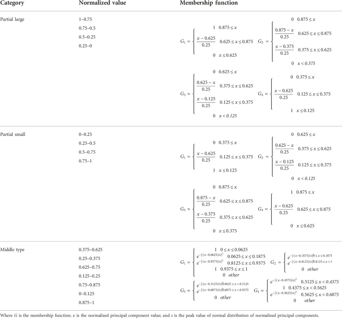
TABLE 4. Membership function table.
2.3.3.4.2 Membership matrix of fractured wells
We can get different membership function form of the principal component factors through the existing m fracturing wells of geological and engineering parameters dimension reduction after principal component factors and yield of fitting relationship. The membership is divided into class I, II, III, and IV level grades, and into slants big, partial, small, and middle-type membership function expression, respectively. The n principal component factors of m fractured wells were substituted into the membership function expression of four grades to obtain m n ×4 membership matrix Hi.
where Hi is the membership matrix; hij is the membership degree of different principal components, and is dimensionless.
2.3.2.5 Fuzzy comprehensive evaluation
where Di is the fuzzy set of comprehensive evaluation of the ith fractured well; and dj is the fuzzy comprehensive evaluation value of different principal components of fractured wells.
where fi is the fuzzy comprehensive score of the ith fractured well.
2.3.3 Optimizing construction parameters
2.3.3.1 Orthogonal experimental design
Orthogonal experiment design, and its analysis of the variance method and intuitive analysis are based on probability theory, mathematical statistics, linear algebra theory of scientific arrangement of the test scheme, and the correct analysis of the test results. Meanwhile, the qualitative index quantitatively determines the parameters of the influence of trend, primary and secondary order, and significant degree to obtain a mathematical optimization method as quickly as possible. By introducing the method of orthogonal experimental design and using the “orthogonal table” to arrange the multi-factor experimental schemes, the intrinsic essential laws contained in a large number of schemes are reflected by a limited number of typical and representative schemes, and the influence trend, primary and secondary order, and the significance degree of parameters on cumulative yield can be quantitatively determined (Zeng et al., 2012). In addition, an orthogonal test can eliminate part of the interference caused by test errors and the results are easy to analyze (Dai et al., 2022).
The target block of the shale oil fracturing engineering parameters of horizontal wells can be optimized and compared through random forest algorithm optimization of fluid, quartz sand proportion, shut in well time/d, sand amount per meter and slippery water ratio, average cluster spacing, the average displacement. These seven factors can influence the production of cumulative gain according to the factors to select the four levels (Table 5). We use a four-level experimental design, and therefore the Lα(4β) orthogonal table should be selected. There are seven factors in the experiment. If the interaction between the factors is not considered, then the orthogonal table with β≥7 should be selected. L216(47) is the minimum Lα(4β) orthogonal table meeting the condition of β≥7. The orthogonal table was used to conduct the 12-month cumulative production experiment, and the influence of various factors on the cumulative production was investigated, from which the optimal parameter scheme of horizontal well was obtained.
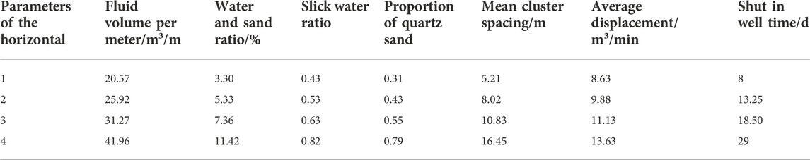
TABLE 5. Factor level table of horizontal well fracturing parameter optimization experiment.
Through the orthogonal design, 216 simulation schemes can be used to complete 47=16384 simulation schemes. This greatly reduces the simulation workload and is conducive to improving the efficiency.
2.3.3.2 Procedure for selecting the construction parameters
1) The random forest method was used to screen out the main controlling factors that affect the production of m training fracturing wells.
2) Principal component analysis was used to reduce the dimensions of the selected main control factors into n principal components to obtain a principal component matrix with m rows and n columns.
3) Based on the relationship between the principal component data of different columns in the principal component matrix and the yield, the membership function is divided into four parts. The analytical formula of different intervals is obtained for each part according to the form of membership function.
4) The membership matrix of m n rows and four columns of fractured wells can be calculated by substituting the data of each column in the principal component matrix of m rows and n columns into the membership function in Step 3.
5) Based on the relationship between the principal component data of different columns in the principal component matrix and the production, the weight values of the main control factors of shale oil fractured horizontal wells can be obtained using random forest.
6) The fuzzy comprehensive scores of different fractured horizontal wells can be obtained using Eqs 17, 18.
7) The function model of main control factors and production was obtained by fitting the relationship between the fuzzy comprehensive score of different fractured horizontal wells and production.
8) A fracturing construction parameter scheme for U test fractured horizontal wells based on the principle of positive price experiment was designed according to the range of fracturing construction parameters.
9) The schemes in Step 8 are evaluated and compared using the fuzzy comprehensive evaluation model. The scheme with the highest score is the optimized construction parameter. The predicted production of the optimized test fractured horizontal well can be obtained by substituting the score into the function model in Step 7.
3 Results and analysis
3.1 Model establishment
3.1.1 Weight determination
Based on the data in Supplementary Table S1, the principal components of different fractured horizontal wells were applied to determine the weights by the random forest algorithm. The results are shown in Figure 2, which shows that the weight of principal components reaches 0.63.
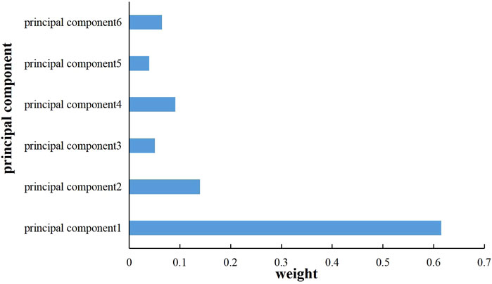
FIGURE 2. Principal component weight values.
3.1.2 Fuzzy comprehensive evaluation
The principal component data of different fractured wells in Supplementary Table S2 were substituted into the membership function and the fuzzy set results of comprehensive evaluation of different fractured horizontal wells were obtained using Eqs 16, 17, as shown in Supplementary Table S3. The fuzzy comprehensive scores of different fractured horizontal wells can be obtained by substituting the fuzzy set data of comprehensive evaluation of different fractured horizontal wells in Supplementary Table S3 into Eq. 18. Figure 3 shows the fitting result of the score and 12-month kilometer cumulative production obtained by fitting the score to the 12-month kilometer cumulative production. Figure 4 is the fitting result of the score obtained without dimension reduction and the 12-month kilometer cumulative production. It can be obtained by comparison that the model accuracy is higher and the fitting effect is better after dimension reduction. Therefore, the rationality of the proposed method is fully illustrated.
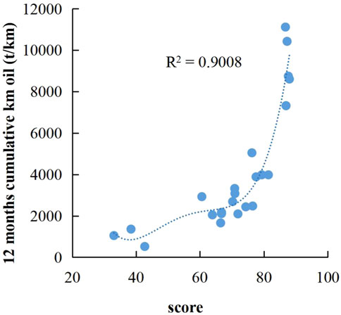
FIGURE 3. Fitting results after reducing dimensionality.
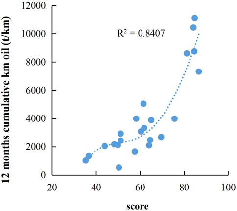
FIGURE 4. Fitting results without reducing dimensionality.
3.2 Model verification
After reducing the dimensionality of the main control factor data of well W24 by principal components, the data were substituted into Eqs 15–17 to obtain the fuzzy comprehensive score and fitted to obtain the predicted production. A comparison between the actual production and the predicted production results is shown in Table 6. It can be found from this that the relative error of the prediction results is 4.8%, which verifies the rationality of the model in this paper.
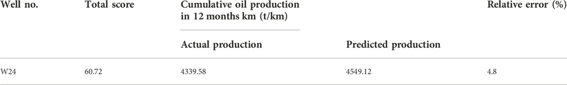
TABLE 6. Comparison between the actual yield and the model’s prediction results.
3.3 Field application
The data of the L216 (47) orthogonal test design scheme can be substituted into the established fuzzy comprehensive evaluation model to predict the output under different construction parameter combinations, as shown in Table 7, which lists the yield prediction results after optimizing parameter combination under 216 simulation schemes. It can be seen that under different construction parameter combinations, the predicted 12-month cumulative production of km varies significantly from 2588.81 t/km to 10742.54 t/km. This shows that the optimization of construction parameters matching with the reservoir can significantly increase production. The optimal No. 147 scheme is selected for construction and the cumulative output of 12 months km is 10144.7 T. The cumulative yield over the 12 months prior to parameter optimization (Table 1) was significantly improved.
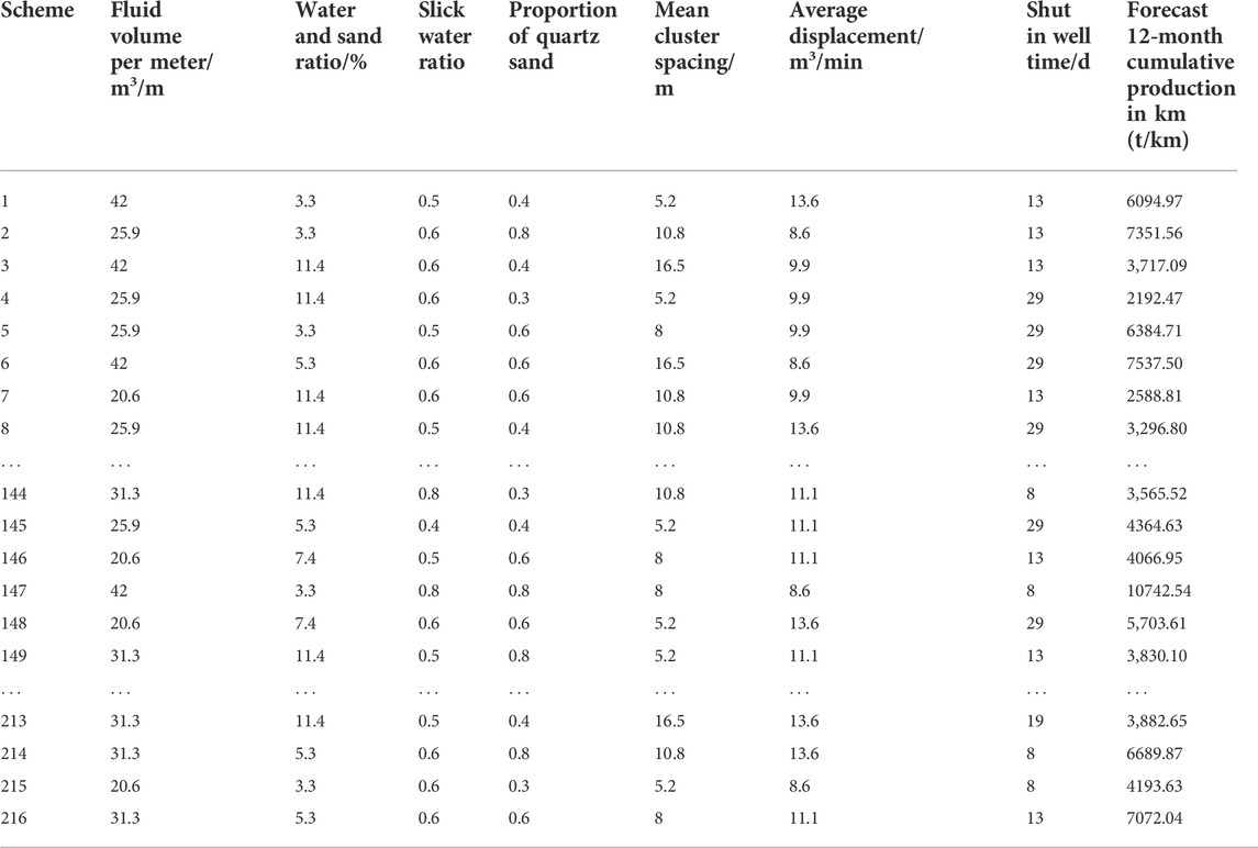
TABLE 7. Design scheme of the orthogonal experiment.
Finally, we compare typical wells (The results are shown in Table 8): wells w24 (before optimization) and w25 (after optimization) are two adjacent horizontal wells of similar length on the same platform. The production of well w25 was 2.34 times that of well w24 after the implementation of optimized parameters, and the stimulation effect was obvious (Figure 5). A comparison of the construction scale of the two wells shows that the fluid volume, the proportion of slick water, the proportion of quartz sand, and the cluster spacing of well w25 are increased, while the cluster spacing and the average displacement are decreased. This shows that the production can be significantly increased by optimizing the construction parameters.
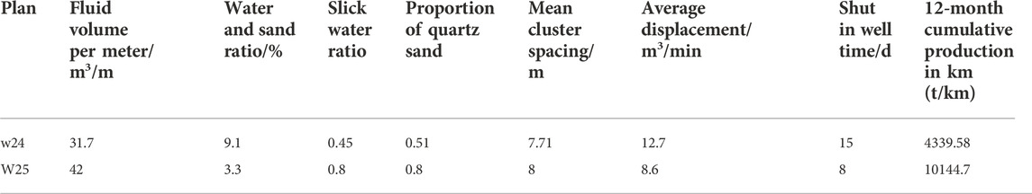
TABLE 8. Comparison table of the optimization parameters and construction effect.

FIGURE 5. Production comparison of W24 and W25.
4 Conclusion
1) Using the random forest method, the main controlling factors of the production of fractured horizontal wells in block W are, successively, the brittleness index (mineral), sand-liquid ratio, quartz sand proportion, S1, soaking length, meter liquid volume, angle between wellbore and principal stress direction, total length of fracturing stage, OSI, natural gamma ray, and so on. Among them, the brittleness index (mineral) has a far greater impact on the yield than other main controlling factors, with an importance of 0.36.
2) After reducing the dimensionality of the 16 original input variables through principal components, the first six principal components extracted contain most of the information of the original variables and these principal components are linearly independent. Selecting the first six principal components as input parameters of the model can reduce noise and error. The R2 value of the model after reducing dimensionality is 0.9 and that of the model without reducing dimensionality is only 0.84.
3) The fuzzy comprehensive evaluation yield model based on principal component analysis and random forest algorithm that we established in this paper shows that the average relative error of the test well is 4.8%, which verifies the rationality of the model in this paper.
4) Compared with adjacent wells, the fluid volume, slippage water proportion, quartz sand proportion, and cluster spacing of the fractured horizontal well in W25 all increased after optimized parameters, while the cluster spacing and average displacement decreased. W25 well was 2.34 times more productive than the offset well. This shows that the production can be significantly increased by optimizing the construction parameters.
Data availability statement
The raw data supporting the conclusion of this article will be made available by the authors, without undue reservation.
Author contributions
DL conceived and designed the experiments; YL and YJ performed the experiments; XL, GX, ZT, LM, CZ, WJ, SX, ZD, TH, ZY, and LY wrote the paper.
Funding
This research was supported by the Natural Science Foundation of China (Grant No. U21A20105).
Conflict of interest
XL, DL, YJ, YL, XG, ZT, CZ, LM, WJ, SX, ZD, and TH were employed by PetroChina Dagang Oilfield Company.
The remaining authors declare that the research was conducted in the absence of any commercial or financial relationships that could be construed as a potential conflict of interest.
Publisher’s note
All claims expressed in this article are solely those of the authors and do not necessarily represent those of their affiliated organizations, or those of the publisher, the editors and the reviewers. Any product that may be evaluated in this article, or claim that may be made by its manufacturer, is not guaranteed or endorsed by the publisher.
Supplementary material
The Supplementary Material for this article can be found online at: https://www.frontiersin.org/articles/10.3389/feart.2022.1015107/full#supplementary-material
References
Chen, R., and Min, M. (2022). Random forest algorithm based on PCA and hierarchical selection in Spark[J]. Comput. Eng. Appl. 58 (06), 118–127.
Dai, S., Wang, H., An, S., and Yuan, L. (2022). Mechanical properties and microstructural characterization of metakaolin geopolymers based on orthogonal tests. Materials 15 (8), 2957. doi:10.3390/ma15082957
Deng, H., Sheng, G., Zhao, H., Meng, F., Zhang, H., Ma, J., et al. (2022). Integrated optimization of fracture parameters for subdivision cutting fractured horizontal wells in shale oil reservoirs. J. Petroleum Sci. Eng. 212, 110205. doi:10.1016/j.petrol.2022.110205
Duplyakov, V. M., Morozov, A. D., Popkov, D. O., Shel, E., Vainshtein, A., Burnaev, E., et al. (2022). Data-driven model for hydraulic fracturing design optimization. Part II: Inverse problem. J. Petroleum Sci. Eng. 208, 109303. doi:10.1016/j.petrol.2021.109303
Duplyakov, V., Morozov, A., Popkov, D., Vainshtein, A., Osiptsov, A., Burnaev, E., et al. (2020). “Practical aspects of hydraulic fracturing design optimization using machine learning on field data: Digital database, algorithms and planning the field tests[C],” in SPE Symposium: Hydraulic Fracturing in Russia. Experience and Prospects.
Guo, D., Kang, Y., Wang, Z., Zhao, Y., and Li, S. (2022). Optimization of fracturing parameters for tight oil production based on genetic algorithm. Petroleum 8 (2), 252–263. doi:10.1016/j.petlm.2021.11.006
Guo, J., Lu, Q., Zhu, H., Wang, Y., and Ma, L. (2015). Perforating cluster space optimization method of horizontal well multi-stage fracturing in extremely thick unconventional gas reservoir. J. Nat. Gas Sci. Eng. 26, 1648–1662. doi:10.1016/j.jngse.2015.02.014
He, J., Wen, X., Nie, W.-L., Li, L., and Yang, J. (2020). Prediction of fracture zones using random forest algorithm [J]. Oil Geophys. Prospect. 55 (1), 161–166.
Hu, S., Zhao, W., Hou, L., Yang, Z., Zhu, R., Wu, S., et al. (2020). Development potential and technical countermeasures of continental shale oil in China[J]. Petroleum Explor. Dev. 47 (04), 819–828.
Hui, G., Chen, S., He, Y., Wang, H., and Gu, F. (2021). Machine learning-based production forecast for shale gas in unconventional reservoirs via integration of geological and operational factors. J. Nat. Gas Sci. Eng. 94, 104045. doi:10.1016/j.jngse.2021.104045
Lei, J., Ju-Hua, L., and Jia-Lin, X. (2020). Application of random forest algorithm in multi-stage fracturing of shale gas field [J]. Petroleum Geol. oilfield Dev. daqing 39 (06), 168–174.
Li, Yongxiang, Cao, Zeyang, and Yang, Zhiwei (2020). Evaluation of maintenance support ability of maintenance personnel based on principal component analysis[J]. Mod. Def. Technol. 48 (04), 110–116.
Li-Yang, S., Wang, J.-w., and Chang-yin, L. (2022). Intelligent fracturing design method for horizontal Wells based on BP-GA algorithm[J]. Fault block oil field 29 (03), 417–421.
Ma, C., Xing, Y., Qu, Y., Cheng, X., and Wu, H. (2022). A new fracture parameter optimization method for the horizontal well section of shale oil[J]. Front. Earth Sci. 10, 2296–6463.
Ma, J., shi, S., jin, C., Zhang, J., He, X., Li, X., et al. (2021). Optimization of fracture design for horizontal wells in Mahu region based on machine learning. J. Shenzhen Univ. Sci. Technol. 38 (06), 621–627. doi:10.3724/sp.j.1249.2021.06621
Moradidowlatabad, M., and Jamiolahmady, M. (2018). The performance evaluation and design optimisation of multiple fractured horizontal wells in tight reservoirs. J. Nat. Gas Sci. Eng. 49, 19–31. doi:10.1016/j.jngse.2017.10.011
Nguyen-Le, V., and Shin, H. (2019). Development of reservoir economic indicator for Barnett Shale gas potential evaluation based on the reservoir and hydraulic fracturing parameters. J. Nat. Gas Sci. Eng. 66, 159–167. doi:10.1016/j.jngse.2019.03.024
Pu, X., Han, W., Zhou, L., Chen, S., Zhang, W., Shi, W., et al. (2015). Lithologic characteristics and geological significance of fine-grained facies area of kong2 high level system domain in cangdong sag, huanghua depression[J]. China Pet. Explor. 20 (05), 30–40.
Rahmanifard, H., and Plaksina, Q., (2018). Application of fast analytical approach and AI optimization techniques to hydraulic fracture stage placement in shale gas reservoirs. J. Nat. Gas. Sci. Eng. 52, 367–378. doi:10.1016/j.jngse.2018.01.047
Ren, J., Liao, Q., Lu, G., Fu, L., Zhou, J., Qi, P., et al. (2010). Tectonic deformation pattern and evolution process analysis in huanghua depression[J]. Tect. metallogeny 34 (04), 461–472.
Rodriguez, R. S., and Soeder, D. J. (2015). Evolving water management practices in shale oil & gas development. J. Unconv. Oil Gas Resour. 10, 18–24. doi:10.1016/j.juogr.2015.03.002
Shahkarami, A., Ayers, K., Wang, G., and Ayers, A. (2018). “Application of machine learning algorithms for optimizing future production in marcellus shale, case study of southwestern Pennsylvania[C],” in SPE/AAPG Eastern Regional Meeting.
Syed, F. I., Alnaqbi, S., Muther, T., Dahaghi, A. K., and Negahban, V. (2022). Smart shale gas production performance analysis using machine learning applications[J]. Petroleum Res. Engl. 7 (1), 21–31.
Tan, C., Yang, J., Cui, M., Hua, W., Chunqiu, W., Hanwen, D., et al. (2021). Lithosphere, 2021.Fracturing productivity prediction model and optimization of the operation parameters of shale gas well based on machine learning[J]
Wang, J., Singh, A., Liu, X., Rijken, M., Tan, Y., and Naik, S. (2022). Efficient prediction of proppant placement along a horizontal fracturing stage for perforation design optimization. SPE J. 27 (02), 1094–1108. doi:10.2118/208613-pa
Wang, L., Yao, Y., Wang, K., Adenutsi, C. D., Zhao, G., and Lai, F. (2022). Data-driven multi-objective optimization design method for shale gas fracturing parameters. J. Nat. Gas Sci. Eng. 99, 104420. doi:10.1016/j.jngse.2022.104420
Wang, S., and Chen, S. (2019). Insights to fracture stimulation design in unconventional reservoirs based on machine learning modeling. J. Petroleum Sci. Eng. 174, 682–695. doi:10.1016/j.petrol.2018.11.076
Xiao, C., Zhang, S., Ma, X., Zhou, T., and Li, X. (2022). Surrogate-assisted hydraulic fracture optimization workflow with applications for shale gas reservoir development: A comparative study of machine learning models. Nat. Gas. Ind. B 9 (3), 219–231. doi:10.1016/j.ngib.2022.03.004
Xie, Jijian, and Liu, Chengping (2013). Fuzzy mathematics method and its application[M]. Wuhan: Huazhong University of Science and Technology Press.
Zeng, F., Guo, J., He, S., and Zeng, L. (2012). Optimization of fracture parameters for fractured horizontal Wells in tight sandstone gas reservoirs [J]. Nat. gas industry 32 (11), 54–58.
Keywords: shale oil, random forest, principal component analysis, fuzzy comprehensive evaluation, orthogonal test design, construction parameters optimization
Citation: Liu X, Li D, Jia Y, Liyong Y, Xiaoting G, Tao Z, Ziwei C, Mao L, Juan W, Xiangyun S, Donghua Z, Hongxia T, Yulin L and Yu Z (2023) Optimizing construction parameters for fractured horizontal wells in shale oil. Front. Earth Sci. 10:1015107. doi: 10.3389/feart.2022.1015107
Received: 09 August 2022; Accepted: 30 August 2022;
Published: 09 January 2023.
Edited by:
Jinze Xu, University of Calgary, CanadaReviewed by:
Huzhen Wang, Northeast Petroleum University, ChinaQi Zhang, China University of Geosciences Wuhan, China
Copyright © 2023 Liu, Li, Jia, Liyong, Xiaoting, Tao, Ziwei, Mao, Juan, Xiangyun, Donghua, Hongxia, Yulin and Yu. This is an open-access article distributed under the terms of the Creative Commons Attribution License (CC BY). The use, distribution or reproduction in other forums is permitted, provided the original author(s) and the copyright owner(s) are credited and that the original publication in this journal is cited, in accordance with accepted academic practice. No use, distribution or reproduction is permitted which does not comply with these terms.
*Correspondence: Xuewei Liu, dg_liuxwei@petrochina.com.cn; Li Yulin, 1732875754@qq.com