 Heng Wang
 Yungui Xu
 Shuhang Tang1,2
 Weiping Cao
 Xuri Huang
95% of researchers rate our articles as excellent or good
Learn more about the work of our research integrity team to safeguard the quality of each article we publish.
Find out more
ORIGINAL RESEARCH article
Front. Earth Sci. , 07 July 2023
Sec. Environmental Informatics and Remote Sensing
Volume 11 - 2023 | https://doi.org/10.3389/feart.2023.1153619
This article is part of the Research Topic Advances and Applications of Artificial Intelligence in Geoscience and Remote Sensing View all 14 articles
Well log prediction while drilling estimates the rock properties ahead of drilling bits. A reliable well log prediction is able to assist reservoir engineers in updating the geological models and adjusting the drilling strategy if necessary. This is of great significance in reducing the drilling risk and saving costs. Conventional interactive integration of geophysical data and geological understanding is the primary approach to realize well log prediction while drilling. In this paper, we propose a new artificial intelligence approach to make the well log prediction while drilling by integrating seismic impedance with three neural networks: LSTM, Bidirectional LSTM (Bi-LSTM), and Double Chain LSTM (DC-LSTM). The DC-LSTM is a new LSTM network proposed in this study while the other two are existing ones. These three networks are thoroughly adapted, compared, and tested to fit the artificial intelligent prediction process. The prediction approach can integrate not only seismic information of the sedimentary formation around the drilling bit but also the rock property changing trend through the upper and lower formations. The Bi-LSTM and the DC-LSTM networks achieve higher prediction accuracy than the LSTM network. Additionally, the DC-LSTM approach significantly promotes prediction efficiency by reducing the number of training parameters and saving computational time without compromising prediction accuracy. The field data application of the three networks, LSTM, Bi-LSTM, and DC-LSTM, demonstrates that prediction accuracy based on the Bi-LSTM and DC-LSTM is higher than that of the LSTM, and DC-LSTM has the highest efficiency overall.
During the drilling process, reliable prediction of the rock properties of the geological formation below the drill bit is of great significance. If well logs can be effectively obtained within a certain depth range below the drill bit, it can surely help to improve the drilling process with lower risk and optimal strategy. Researchers have proposed various methods for well log prediction while drilling (Wang, 2017; Tamim et al., 2019). Wang (2017) established a 3D model by analyzing the drilling core, rock chip, and seismic data. The well log curve values below the drilling bit along the borehole trajectory are predicted based on the 3D model. Tamim et al. (2019) constructed a Bayesian classifier using well logs as the classification target. With the posterior probability calculated with prior distribution and conditional probability, the spatial distribution of well logs can be predicted. However, the actual geological formations are non-homogeneous and complex. The logging curve values show great fluctuations with depth even when the sampling interval of the well log is small. The mapping relationships between different data points are strongly non-linear, and the traditional methods are not able to effectively predict the actual formation changes.
Predicting rock property with geophysical data is often a non-linear problem in many cases. Describing the intrinsic relationship between properties and their geophysical responses using explicit mathematical or physical equations can be challenging. However, machine learning has shown great potential in recent years, as it can describe these relationships with network parameters by using a large number of training datasets. Examples of relevant machine learning applications include geological parameter estimation (Ahmed Ali Zerrouki and Baddari, 2014; Iturrarán-Viveros and Parra, 2014), lithology discrimination (Wang et al., 2014; Silva et al., 2015), and stratigraphic boundary determination (Singh, 2011; Silversides et al., 2015). In recent years, there has been a surge of research on well log prediction, resulting in significant improvements in performance (Rolon et al., 2009; Alizadeh et al., 2012; Mo et al., 2015; Long et al., 2016; Salehi et al., 2017).
The well log prediction methods discussed above use fully connected neural networks (FCNN) to construct a point-to-point mapping. However, FCNN shows less effectiveness in characterizing the trend of the data because it cannot capture the relations between the point data of well log at different depths. This means that the correlation between the rock properties at a shallower depth and those at a deeper depth is ignored, potentially contradicting the sedimentary principles in the geological sense. To fix this problem with FCNN in well log prediction, many researchers have improved FCNN by coupling non-machine learning methods, such as wavelet transform (Adamowski and Chan, 2011) and singular spectrum analysis (Sahoo et al., 2017). However, these improvements are often complex and cumbersome to implement. An alternative way to utilize recurrent neural networks (RNNs) is able to deal the problems (Schuster and Paliwal, 1997). In the RNN structure, there is a self-looping structure within each neural unit, which allows previous information to be retained and used later. Since the information can flow freely in the RNN, well log prediction with this method integrates the intrinsic connection between different logs and the overall trend with depth, which follows geological principles.
Long Short-Term Memory Neural Networks (LSTM), an advanced form of RNN, have become widely utilized in the deep learning community for various tasks. LSTM incorporates gate structures within each automatic cycle structure to mimic biological neurons’ information conduction patterns, thereby storing more long-term sequential information without additional tuning. This attribute has facilitated LSTM’s extensive use in natural language processing (Deng et al., 2019), machine translation (Lokeshkumar et al., 2020), and speech recognition (Graves and Jaitly, 2014). Moreover, RNNs and LSTMs have also found applications in the field of hydrology to deal with time series data-related problems (da Silva and Saggioro, 2013), and some researchers have used LSTM to generate logs (Jin, 2018).
In the case of well log prediction while drilling, Wang et al. (2020) employed the LSTM model, whereas Shan et al. (2021) utilized the CNN-LSTM hybrid model to achieve the goal. Both methods employed neighboring well logs to predict the logs at the undrilled segment, resulting in successful outcomes. However, when neighboring wells are too distant (as in the case of sparse neighboring wells) and well correlation is weak, the prediction results can become biased. In certain scenarios, prediction may not be possible due to the unavailability of well logs from neighboring wells at the prediction depth.
This study proposes a novel approach for well log prediction while drilling, utilizing seismic impedance and three different artificial intelligence networks: the LSTM network and its two derivative networks, namely, the Bi-LSTM and the newly developed Double Chain LSTM (DC-LSTM). The proposed methodology effectively integrates seismic impedance constraints for well log prediction. The results demonstrate that the two derivative networks outperform the LSTM network in terms of prediction accuracy. Additionally, the DC-LSTM network exhibits superior computational efficiency as compared to the Bi-LSTM network, owing to the reduction in the number of network parameters and consequently the computing time, while maintaining prediction accuracy. A practical case study is conducted to verify the effectiveness of the proposed methodology.
The acquisition of well logs is traditionally carried out after drilling, while well log prediction while drilling refers to the real-time estimation of well logs at a certain depth below the drill bit during the drilling process. This paper presents a workflow for such prediction, as depicted in Figure 1. The known observed logs are shown in red, whereas the logs yet to be predicted are shown in blue. The seismic impedance obtained through seismic inversion is utilized as input data for the training and prediction of well logs using three different networks, as outlined in Table 1.
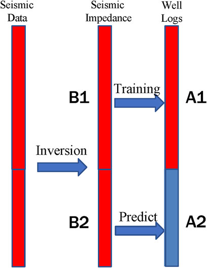
FIGURE 1. Workflow of data procession. (Red means known value and blue means unknown value).
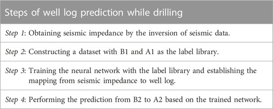
TABLE 1. The steps of the work.
The LSTM neural network (Hochreiter and Schmidhuber, 1997) is a specialized type of recurrent neural network (RNN) designed to capture long-term dependencies within sequential data. This makes it particularly suitable for processing well logs, which are a type of sequential data with a relatively small sampling interval. A significant characteristic of well logs is the representation of long-term depth trends within a large depth interval, which can play an essential role in prediction tasks. Unfortunately, these trends are often overlooked in existing models. However, LSTM’s ability to retain information with long-term dependencies from previous, more distant steps allows it to capture and incorporate these trends into its predictions. As a result, LSTM represents an effective tool for well log prediction.
Figure 2 illustrates the architecture of the LSTM network. The inputs to the network are denoted by
FIGURE 2. The architecture of the LSTM. (Each green box stands for one LSTM unit).
The Bi-LSTM neural network (Graves and Schmidhuber, 2005) represents a variant of the LSTM architecture that incorporates two parallel LSTMs: one running forward along the input sequence, and another running backward in reverse order. By exploiting both the past and future context of the input data, the Bi-LSTM model can capture more comprehensive and accurate representations of sequential data. Specifically, the forward and backward LSTMs compute hidden state vectors in opposite directions, and the final output of the network is produced by combining the two LSTM’ outputs with appropriate weights in the output layer. A diagram of the Bi-LSTM structure is presented in Figure 3.

FIGURE 3. The architecture of the BiLSTM.
In Figure 3, the input is denoted by
where a ⊗ is a matrix operator, which is utilized to couple
Figures 4, 5 present the prediction framework using a Bi-LSTM network for mapping the relationship between well logs and seismic impedance. The prediction framework is comprised of three layers, namely, the input layer, the output layer, and the hidden layer. The network is trained using the training set to obtain the mapping relationship between the log segment of the well and seismic impedance. The seismic impedance within the undrilled well segment is then used to predict well logs.
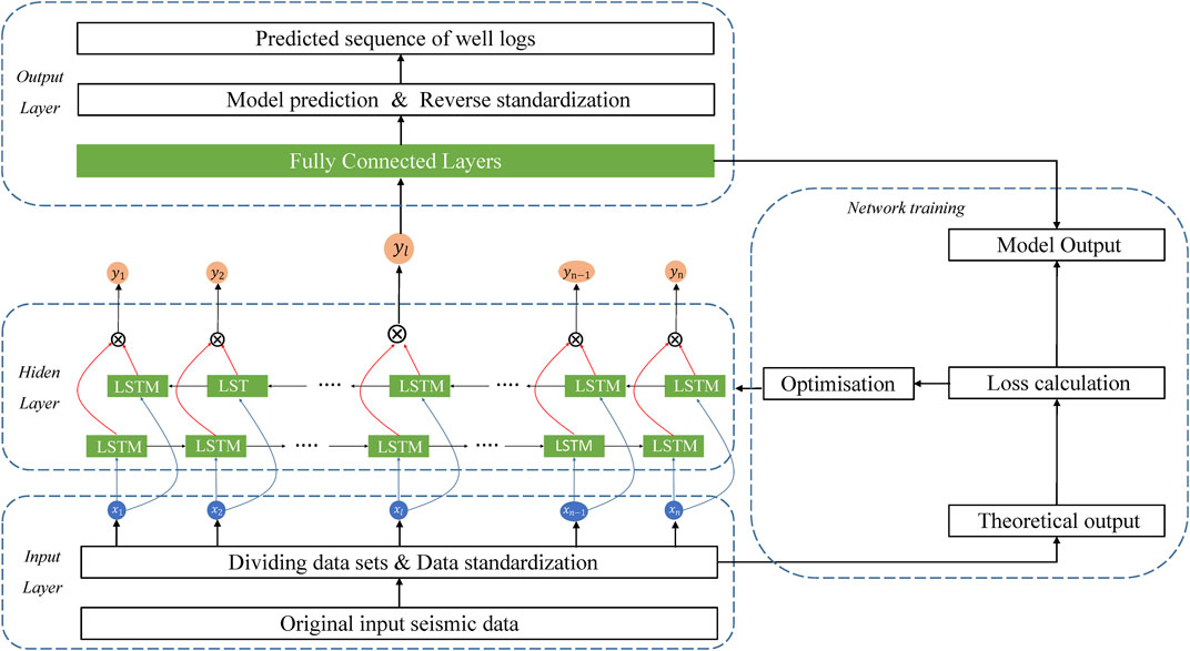
FIGURE 4. Prediction framework of Bi-LSTM network.
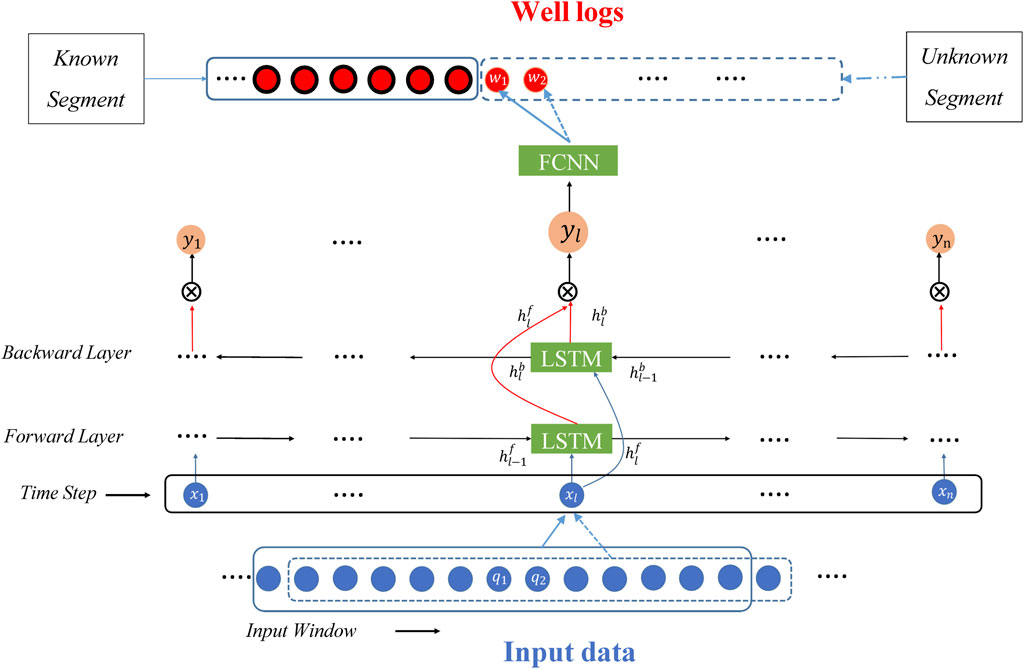
FIGURE 5. Flow chart for prediction of Bi-LSTM network.
In Figure 5, the model is trained using well logs observed from the drilled segment and the corresponding seismic impedance to optimize the network. The trained model is subsequently used to predict log values of the well segment below the training data along the well trajectory. The input window specifies the length of the input seismic impedance sequence to the network, and the input window length should be consistent between the training and prediction phases. In the current example,
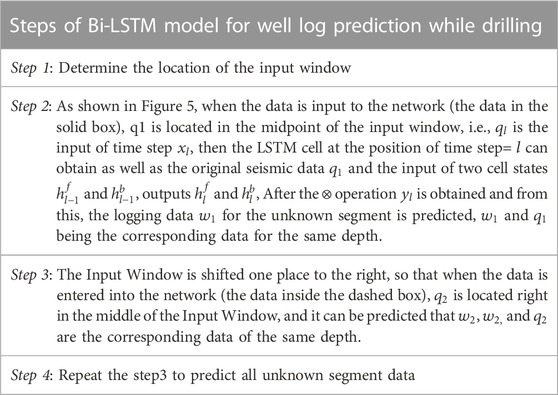
TABLE 2. The specific steps of the prediction phase.
The Bi-LSTM model utilized for well log prediction while drilling entails numerous prediction parameters. Specifically, the final output of a Bi-LSTM layer is expressed as a set of vectors, denoted as
The DC-LSTM network is an optimized network that aims to enhance the computational efficiency in well log prediction while drilling in comparison to the Bi-LSTM model. As shown in Figure 6, DC-LSTM divides the input sequence, represented by
FIGURE 6. The architecture of the Double-chain network.
Figures 7, 8 depict the prediction process with DC-LSTM, which is a simplified and more efficient version of Bi-LSTM in well log prediction while drilling. As illustrated in Figure 7, DC-LSTM replaces Bi-LSTM in the hidden layer, resulting in a simpler overall structure. Furthermore, Figure 8 shows that DC-LSTM requires only n+1 LSTM units, whereas Bi-LSTM utilizes 2n LSTM units. This reduces the number of parameters and improves computational efficiency. Importantly,
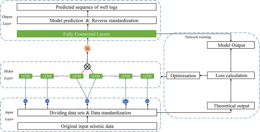
FIGURE 7. Prediction framework of DC-LSTM network.
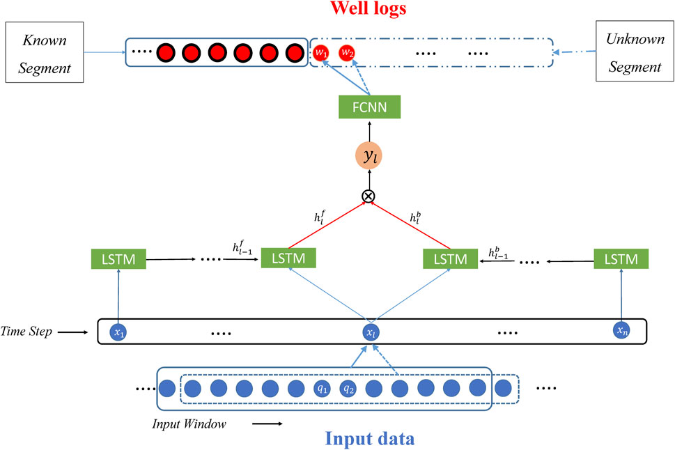
FIGURE 8. Flow chart for prediction of DC-LSTM.
The steps of prediction with DC-LSTM are largely analogous to those outlined in Table 2 for Bi-LSTM. The only difference is that DC-LSTM divides the input sequence
In this part, we present the results of well log prediction while drilling using seismic impedance with the LSTM, Bi-LSTM, and DC-LSTM.
In this experiment, a pilot area of an oil field in East China is selected for well log prediction. Two wells and a seismic impedance cube in the area are used in this experiment (see Figure 9). The two wells have four logs for testing, density (DEN), natural gamma ray (GR), compensated neutron log (CNL), and induction (CON).
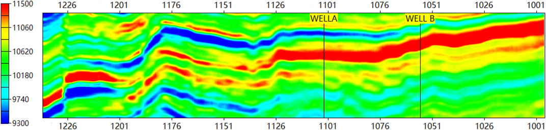
FIGURE 9. Seismic impedance profile of input data.
Before the prediction with the three networks, two data preprocessing tasks, data cleaning, and standardization are required.
Data cleaning (Zhang et al., 2015) aims to improve the data quality of input data. Common problems with logs, such as invalid and missing values, are cleared. Check on the data value range are necessary as well. Any data point, falling outside the normal range, logically unreasonable, or contradictory, is also cleared.
The purpose of data standardization is to centralize data values so that the characteristics of each type of data are balanced. Data standardization also reduces the disturbance of anomalous values that still exist after data cleaning. This paper uses the z-score normalization method (Hrynaszkiewicz, 2010) to standardize input data standardization, expressed in the equations below,
where
The problem discussed in this paper is called the ‘regression task’ in the field of the neural network, and the common loss functions of the regression task are Mean Square Error (MSE), Root Mean Square Error (RMSE), and Mean Absolute Error (MAE). If there are some unusual values (large or small) in the data, these values are more likely to indicate the important geological contrast in rock properties, such as sudden change of lithology, measured acoustic velocity, etc. Therefore, it is necessary to attach more weight on the unusual values. This is achieved by using MSE as the loss function.
MAE and RMSE are used as criteria to evaluate prediction accuracy. MAE is the average of the absolute error between the predicted value and the true value, indicating the true situation of the error, while RMSE is generally used to indicate the deviation between the predicted value and the true value. MAE, MSE, and RMSE are defined as,
where
In this study, the MAE and RMSE of four logs are calculated and averaged to evaluate the performance of different models. However, the value ranges of these four curves are very different, and the value ranges of the same curve in different wells are also different. For the fair evaluation of the results, the true and predicted values of each curve are put together and normalized before calculating the MAE and RMSE, according to the following equation,
where
In this experiment, two wells, namely, Well A (with measured depth ranging from 3220m to 3960 m) and Well B (ranging from 3700 to 4400 m), along with a seismic impedance segment traversing both wells, were utilized as input data (as depicted in Figure 9). The training data set was constructed by incorporating the first 70% of the well log data (the section above the red line shown in Figure 10), along with the corresponding seismic impedance. The remaining 30% of the logs (the section below the red line in Figure 10) and their corresponding seismic impedance were used for blind test validation. The sampling interval for both wells was set to 0.076 m. The input window length for the networks was fixed at 51 neighboring data points, which corresponds to an actual sampling length of 3.876 m. By using seismic impedance, each input window predicts a single well log point at the depth of the middle point of the input window. The window length determines the memory range of the network model during both the training and prediction processes.

FIGURE 10. Logging curves for well A and well B used in training and validation: (A) well A, (B) well B
In this study, the training data set is obtained by dividing the impedance and well logs into segments with a length of 51. The impedance is utilized as the input, while four well logs, including density (DEN), natural gamma ray (GR), compensated neutron log (CNL), and induction (CON) curves, serve as the output. The optimal training parameters, as demonstrated in Table 3, are determined through several rounds of parameter tests.
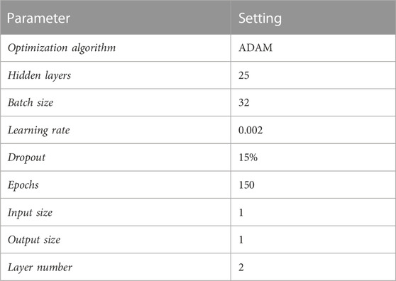
TABLE 3. Training parameter setting.
The training sequences (impedance and well logs) are divided into segments with a length of 51 to produce the training and prediction data set. The impedance is used as the input. Four well logs, including density (DEN), natural gamma ray (GR), compensated neutron log (CNL), and induction (CON) curves, are used as the output. The best results are obtained by using the training parameters shown in Table 3 after a few times of parameter tests.
Figures 11, 12 depict the outcomes of the three methods employed in the analysis of the two wells, where the red and blue curves indicate the predicted and actual values, respectively. As illustrated in these figures, the performance of the LSTM-based method is suboptimal, as it fails to capture the geological changes adequately, leading to inaccurate overall predictions. Conversely, the Bi-LSTM and DC-LSTM methods yield favorable results in both detecting the geological variations in detail and predicting the overall trend.
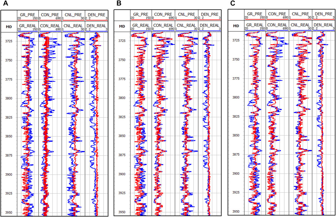
FIGURE 11. Results of the three networks applied to well A: (A) LSTM, (B) Bi-LSTM, (C) DC-LSTM.
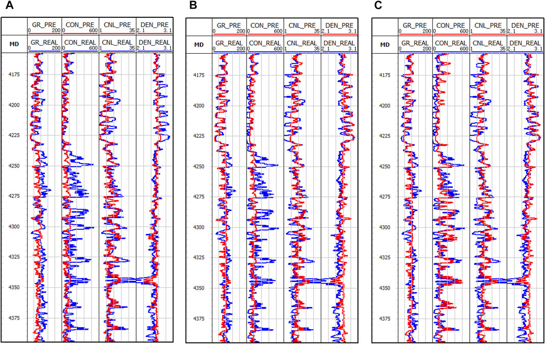
FIGURE 12. Results of the three networks applied to well B: (A) LSTM, (B) Bi-LSTM, (C) DC-LSTM.
Table 4, 5 present the Mean Absolute Error (MAE) and Root Mean Squared Error (RMSE) values of three methods applied to two wells. Figure 13 is a bar chart illustrating the performance of these methods. The results indicate that the MAE and RMSE values of the Bi-LSTM and DC-LSTM models are significantly lower than those of the LSTM model in terms of average value. This finding implies that the predicted values of Bi-LSTM and DC-LSTM are closer to the true values than those of the LSTM model. The MAE and RMSE values of DC-LSTM are similar to those of Bi-LSTM. However, Table 6 shows that using DC-LSTM significantly reduces the time required for model training and prediction.
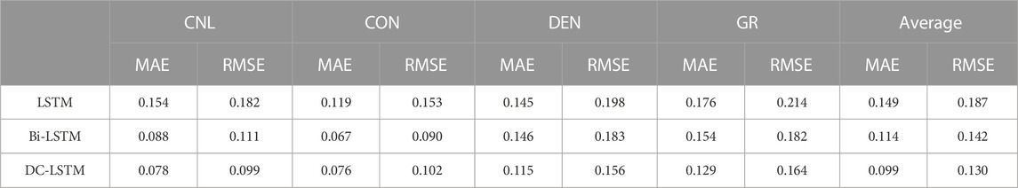
TABLE 4. MAE and RMSE of the three methods applied to well A.
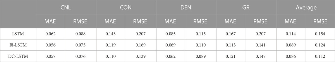
TABLE 5. MAE and RMSE of the three methods applied to well B.
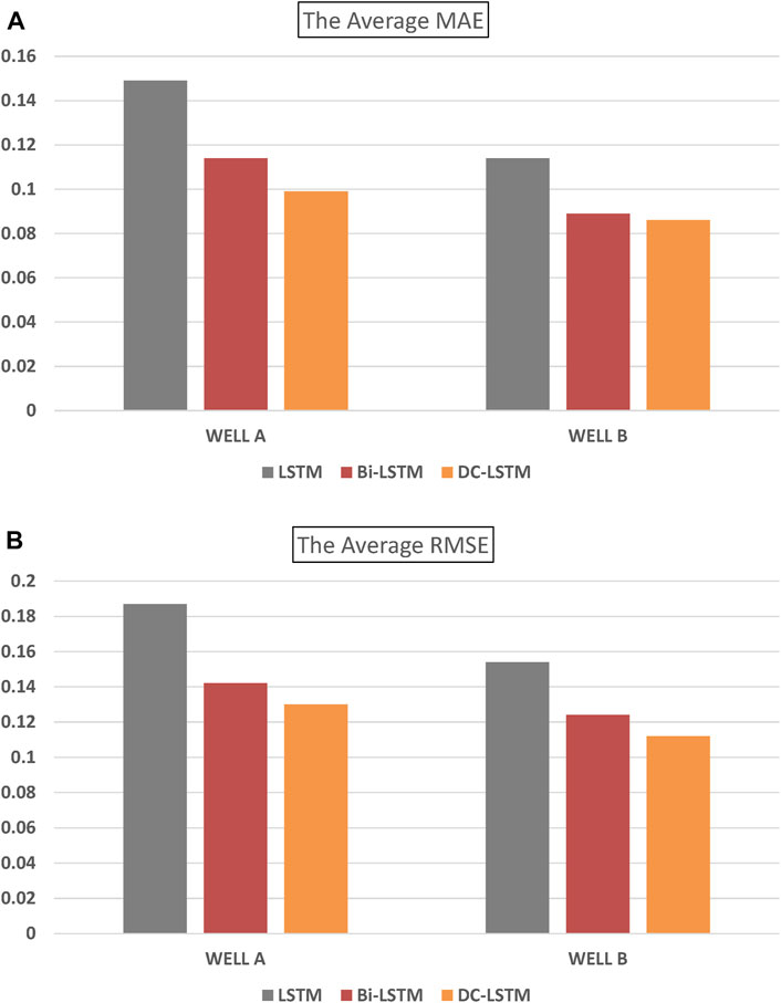
FIGURE 13. The average MAE and RMSE of three methods on three wells: (A) MAE, (B) RMSE.
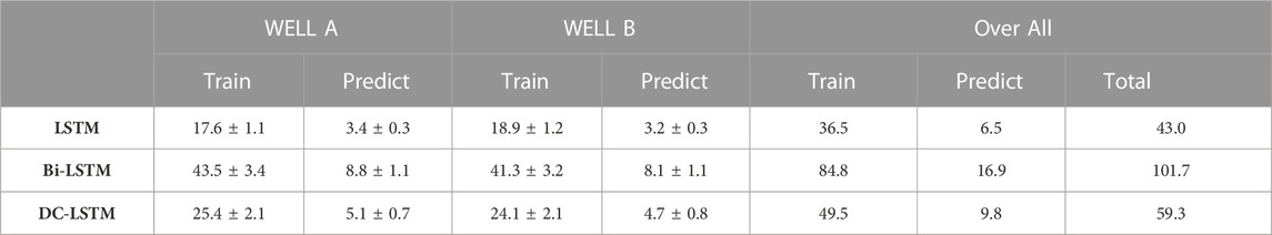
TABLE 6. Time spent on three methods (Unit: seconds).
In well log prediction while drilling, accuracy is a crucial reference factor. In this study, the models are evaluated based on the time spent, using the same personal computer with NVIDIA GPU (GTX 1650 with 4 GB video storage) and the same set of parameters for training and prediction. Table 6 and Figure 14 show the time spent on the models. Results reveal that the running time of the LSTM model is the shortest among the three methods, but its accuracy is the lowest. Bi-LSTM and DC-LSTM models exhibit comparable higher accuracy, with DC-LSTM being more efficient in terms of computational time.
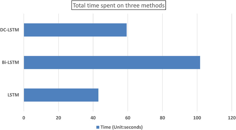
FIGURE 14. Total time spent on three methods.
This paper presents a novel approach for predicting well logs using artificial intelligence while drilling, utilizing seismic impedance and three related LSTM networks. The proposed approach incorporates the constraints of sedimentary formation seismic impedance at the drill bit and the changing trend of impedance through the upper and lower formations. This optimization of the prediction process results in improved computational efficiency. Through experimentation, the Bi-LSTM and DC-LSTM derivative networks are demonstrated to have higher prediction accuracy than the base LSTM. Notably, the DC-LSTM network, developed in this paper, is more efficient in reducing the number of training parameters and computational time without compromising prediction accuracy, as compared to the Bi-LSTM. Field data tests of the three networks were conducted using two wells, and the results demonstrate their effectiveness and efficiency.
The data-driven approach utilizing the three networks is effective for predicting well logs in laterally homogeneous target formations, particularly in the case of clastic sedimentation. However, if the formation exhibits significant lateral heterogeneity, such as fractures and faults near the drilling bits, the prediction accuracy may be compromised. Therefore, the challenge of making reliable predictions under such conditions with limited quality data and rapidly changing trends is an important research topic for the future.
The datasets presented in this article are not readily available because Oilfield sensitive. Requests to access the datasets should be directed to eXVuZ3VpLnh1QG91dGxvb2suY29t.
HW was responsible for the preliminary literature research, the writing of the whole manuscript, and the drawing of the figure. YX and ST were responsible for the late revision and submission of the manuscript. LW, WC, and XH were responsible for providing inspiration and ideas for the manuscript.
National Natural Science Foundation of China: U20B2016. Study on high temperature high pressure seismic rock model and integrated intelligent reservoir characterization methods for a mid-deep reservoir in Yingqiong basin.
LW was employed by Shale Gas Project Management Department of CNPC Chuanqing Drilling Engineering Co., Ltd.
The remaining authors declare that the research was conducted in the absence of any commercial or financial relationships that could be construed as a potential conflict of interest.
All claims expressed in this article are solely those of the authors and do not necessarily represent those of their affiliated organizations, or those of the publisher, the editors and the reviewers. Any product that may be evaluated in this article, or claim that may be made by its manufacturer, is not guaranteed or endorsed by the publisher.
Adamowski, J., and Chan, H. F. (2011). A wavelet neural network conjunction model for groundwater level forecasting. J. Hydrology 407 (1-4), 28–40. doi:10.1016/j.jhydrol.2011.06.013
Ahmed Ali Zerrouki, T. A., and Baddari, K. (2014). Prediction of natural fracture porosity from well log data by means of fuzzy ranking and an artificial neural network in Hassi Messaoud oil field, Algeria. J. Petroleum Sci. Eng. 115, 78–89. doi:10.1016/j.petrol.2014.01.011
Alizadeh, B., Najjari, S., and Kadkhodaie-Ilkhchi, A. (2012). Artificial neural network modeling and cluster analysis for organic facies and burial history estimation using well log data: A case study of the south pars gas field, Persian gulf, Iran. Comput. Geosciences 45, 261–269. doi:10.1016/j.cageo.2011.11.024
da Silva, J. A. C. I., and Saggioro, N. J. (2013). Recurrent neural network based approach for solving groundwater hydrology problems. London, United Kingdom: IntechOpen.
Deng, H., Zhang, L., and Wang, L. (2019). Global context-dependent recurrent neural network language model with sparse feature learning. Neural Comput. Appl. 31 (2), 999–1011. doi:10.1007/s00521-017-3065-x
Graves, A., and Jaitly, N. (2014). Towards end-to-end speech recognition with recurrent neural networks. Beijing, China: International Conference on Machine Learning.
Graves, A., and Schmidhuber, J. (2005). Framewise phoneme classification with bidirectional LSTM networks. Montreal, QC: 2005 IEEE International Joint Conference on.
Hochreiter, S., and Schmidhuber, J. (1997). Long short-term memory. Neural Comput. 9 (8), 1735–1780. doi:10.1162/neco.1997.9.8.1735
Hrynaszkiewicz, I. (2010). A call for BMC Research Notes contributions promoting best practice in data standardization, sharing and publication. BMC Res. notes 3, 235. doi:10.1186/1756-0500-3-235
Iturrarán-Viveros, U., and Parra, J. O. (2014). Artificial Neural Networks applied to estimate permeability, porosity and intrinsic attenuation using seismic attributes and well-log data. J. Appl. Geophys. 107, 45–54. doi:10.1016/j.jappgeo.2014.05.010
Jin, Z. D. C. Y. M. (2018). Synthetic well logs generation via recurrent neural networks. Beijing, China: Petroleum Exploration and Development (4), 629–639.
Lokeshkumar, R., Jayakumar, K., Prem, V., and Nonghuloo, M. S. (2020). Analyses and modeling of deep learning neural networks for sequence-to-sequence translation(Article). Int. J. Adv. Sci. Technol. 29 (5), 3152–3159.
Long, W., Chai, D., and Aminzadeh, F. (2016). Pseudo density log generation using artificial neural network. Anchorage, AK: SPE Western Regional Meeting.
Mo, X., Zhang, Q., and Li, X. (2015). Well logging curve reconstruction based on genetic neural networks. Jilin Changchun, China: Jilin University. College of Geoexploration Science and Technology.
Rolon, L., Mohaghegh, S. D., Ameri, S., Gaskari, R., and McDaniel, B. (2009). Using artificial neural networks to generate synthetic well logs. J. Nat. Gas Sci. Eng. 1 (4-5), 118–133. doi:10.1016/j.jngse.2009.08.003
Sahoo, S., Russo, T. A., Elliott, J., and Foster, I. (2017). Machine learning algorithms for modeling groundwater level changes in agricultural regions of the U.S. U.S. Water Resour. Res. 53 (5), 3878–3895. doi:10.1002/2016wr019933
Salehi, M. M., Rahmati, M., Karimnezhad, M., and Omidvar, P. (2017). Estimation of the non records logs from existing logs using artificial neural networks. Egypt. J. Petroleum 26 (4), 957–968. doi:10.1016/j.ejpe.2016.11.002
Schuster, M., and Paliwal, K. K. (1997). Bidirectional recurrent neural networks. IEEE Trans.45 (11), 2673–2681. doi:10.1109/78.650093
Shan, L., Liu, Y., Tang, M., Yang, M., and Bai, X. (2021). CNN-BiLSTM hybrid neural networks with attention mechanism for well log prediction. J. Petroleum Sci. Eng. 205, 108838. doi:10.1016/j.petrol.2021.108838
Silva, A. A., Neto, I. A. L., Misságia, R. M., Ceia, M. A., Carrasquilla, A. G., and Archilha, N. L. (2015). Artificial neural networks to support petrographic classification of carbonate-siliciclastic rocks using well logs and textural information. J. Appl. Geophys. 117, 118–125. doi:10.1016/j.jappgeo.2015.03.027
Silversides, K., Melkumyan, A., Wyman, D., and Hatherly, P. (2015). Automated recognition of stratigraphic marker shales from geophysical logs in iron ore deposits. Comput. Geosciences 77, 118–125. doi:10.1016/j.cageo.2015.02.002
Singh, U. K. (2011). Fuzzy inference system for identification of geological stratigraphy off Prydz Bay, East Antarctica. J. Appl. Geophys. 75 (4), 687–698. doi:10.1016/j.jappgeo.2011.08.001
Tamim, N., Laboureur, D. M., Hasan, A. R., and Mannan, M. S. (2019). Developing leading indicators-based decision support algorithms and probabilistic models using Bayesian network to predict kicks while drilling. Process Saf. Environ. Prot. Trans. Institution Chem. Eng. Part B 121, 239–246. doi:10.1016/j.psep.2018.10.021
Wang, G., Carr, T., Ju, Y., and Li, C. (2014). Identifying organic-rich Marcellus Shale lithofacies by support vector machine classifier in the Appalachian basin. Comput. GEOSCIENCES 64, 52–60. doi:10.1016/j.cageo.2013.12.002
Wang, J., Cao, J., Liu, Z., Zhou, X., and Lei, X. (2020). Method of well logging prediction prior to well drilling based on long short-term memory recurrent neural network(Article). J. Chengdu Univ. Technol. Sci. Technol. Ed. 47 (2), 227–236. doi:10.3969/j.issn.1671-9727.2020.02.11
Wang, W., Qiu, Z. S., Zhong, H. Y., Huang, W. A., and Dai, W. H. (2017). Thermo-sensitive polymer nanospheres as a smart plugging agent for shale gas drilling operations. J. Xi'an Shiyou Univ. Nat. Sci. Ed. 32 (2), 116–125. doi:10.1007/s12182-016-0140-3
Keywords: machine learning, long short-term memory, well log prediction, drilling bit, seismic impedance, neural networks
Citation: Wang H, Xu Y, Tang S, Wu L, Cao W and Huang X (2023) Well log prediction while drilling using seismic impedance with an improved LSTM artificial neural networks. Front. Earth Sci. 11:1153619. doi: 10.3389/feart.2023.1153619
Received: 29 January 2023; Accepted: 11 April 2023;
Published: 07 July 2023.
Edited by:
Peng Zhenming, University of Electronic Science and Technology of China, ChinaReviewed by:
Jiachun You, Chengdu University of Technology, ChinaCopyright © 2023 Wang, Xu, Tang, Wu, Cao and Huang. This is an open-access article distributed under the terms of the Creative Commons Attribution License (CC BY). The use, distribution or reproduction in other forums is permitted, provided the original author(s) and the copyright owner(s) are credited and that the original publication in this journal is cited, in accordance with accepted academic practice. No use, distribution or reproduction is permitted which does not comply with these terms.
*Correspondence: Yungui Xu, eXVuZ3VpLnh1QG91dGxvb2suY29t
Disclaimer: All claims expressed in this article are solely those of the authors and do not necessarily represent those of their affiliated organizations, or those of the publisher, the editors and the reviewers. Any product that may be evaluated in this article or claim that may be made by its manufacturer is not guaranteed or endorsed by the publisher.
Research integrity at Frontiers
Learn more about the work of our research integrity team to safeguard the quality of each article we publish.