 Yanbo Mai
 Zheng Sheng
 Hanqing Shi1
- 1College of Meteorology and Oceanography, National University of Defense Technology, Nanjing, China
- 2Collaborative Innovation Center on Forecast and Evaluation of Meteorological Disasters, Nanjing University of Information Science and Technology, Nanjing, China
- 3School of Automation, Southeast University, Nanjing, China
- 4Wuxi First Research Institute, Wuxi, China
This paper develops a new method for the diagnosis and prediction of the evaporation duct heights on the sea, which has certain reference significance for the study of the evaporation ducts. Based on traditional diagnostic and predictive models of evaporation duct heights, a new diagnostic model is proposed. By determining the overall Richardson number Rib, the Monin-Obukhov (M-O) length L and the wind speed characteristic parameter u∗, temperature characteristic parameter θ∗ and humidity characteristic parameters q∗ are calculated, and then the evaporation duct height is diagnosed. Taking the diagnosed heights as a time series, and using the support vector regression (SVR) algorithm improved by a simulated annealing operator, then the time series is analyzed by taking three consecutive sample steps as input and the next sample step as output in order to develop an algorithm for predicting future heights. Finally, the prediction results are compared with those from the traditional auto-regressive (AR) algorithm and classical SVR algorithm to identify the advantages and disadvantages of the improved SVR algorithm. The results show that the root-mean-square error (RMSE) of the traditional AR, the classical SVR and the improved SVR algorithms is 0.60, 0.45, and 0.38, and the mean absolute percentage error (MAPE) of the three algorithms is 7.79%, 6.10% and 4.78%, respectively. The prediction error of the improved SVR algorithm is 37% less than that of the traditional AR algorithm and 15% less than that of the classical SVR algorithm, signifying an improvement in its prediction capability.
Introduction
The propagation of electromagnetic waves in the atmosphere is affected not only by absorption and scattering by molecules and aerosol particles but also by refraction (Kang et al., 2014). Abnormal refraction, such as negative refraction, super refraction, and trapping refraction, can cause abnormal propagation of electromagnetic waves (Kang et al., 2014). Under trapping refraction conditions, part of the electromagnetic wave is captured within a certain thickness of atmosphere and propagates back and forth between the upper and lower layers, just like waves propagating in a metal pipe; Regions of atmosphere causing this sort of propagation are called atmospheric ducts (Kang et al., 2014). There are four kinds of atmospheric ducts: surface ducts, surface-based ducts, elevated ducts, and evaporation ducts (Kang et al., 2014). Evaporation ducts often appear close to the sea surface and it is formed by the evaporation of sea water, which leads to the rapid change of humidity in the vertical direction, and then produces the evaporation ducts. The evaporation ducts have an important influence on the propagation of electromagnetic waves, so they are a vital factor affecting the communication systems of ships and low altitude airborne radar (Shi et al., 2019). The height of an evaporation duct refers to its top height, which is numerically equal to the thickness of the evaporation duct layer (Ivanov et al., 2007). It is the key parameter in determining the refractive index profile of the atmosphere in lower layers and has an important reference significance for the propagation loss of electromagnetic waves. Babin et al. (1997) proposed and tested a new model that uses recently refined bulk similarity expressions developed for the determination of the ocean surface energy budget in the Tropical Ocean Global Atmosphere Coupled Ocean-Atmosphere Response Experiment. Tian et al. (2009a) studied the applicability of evaporation duct Model A in Chinese sea areas by using modified refractivity profiles and meteorological data measured during recent years. To evaluate a method for detecting evaporation ducts, Yang et al. (2016) used hydrological and meteorological data from the South China Sea to compare and analyze measured and predicted evaporation duct heights. Babin and Dockery (2002) developed a wave-riding catamaran with a mast-traveling sensor package (profiling buoy) to generate time-averaged modified refractivity (M) profiles that were then compared with those determined from four evaporation duct models based on the surface layer theory of Liu, Katsaros, and Businger (LKB). Burk et al. (2003) investigated the conditions under which atmospheric island wakes form leeward of Kauai, Hawaii, by using idealized numerical simulations and real forecast data from the U.S. Navy's Coupled Ocean-Atmosphere Mesoscale Prediction System (COAMPS). Tian et al. (2009b) analyzed model sensitivity to air-sea temperature difference, wind speed and relative humidity, and studied the applicability of their model in semitropical sea areas using measured data from recent years. Based on a theoretical derivation, Sheng and Huang (2009, 2010) used simulated and measured radar echo data to retrieve evaporation duct parameters, and analyzed the inversion results and the anti-noise capability of the inversion system. Zhang et al. (2016) and Xie et al. (2017) analyzed the variation of arctic polar vortex in the stratosphere, which may affect the generation of atmospheric ducts. Mai et al. (2020) studied the spatiotemporal distribution of atmospheric ducts in Alaska. Li et al. (2014) proposed a non-iterative scheme using multiple regression to produce similar results to those from classical iterative computation. Liu et al. (2019) compared the sensitivity of four evaporation duct prediction models to meteorological factors, and calculated evaporation duct heights using the four models, based on meteorological observations of the South China Sea, providing a theoretical basis and practical experience for future applications. In order to improve the applicability of the Babin model, Yu et al. (2015) performed a theoretical derivation of the model and conducted simulations to analyze its sensitivity to input parameters. Based on atmospheric boundary layer theory, Liu et al. (2001) studied a theoretical formula for estimating the heights of evaporation ducts using similarity theory, with pseudo refractive index as the similarity parameter. Paulus (1985) applied the P-J model of evaporation ducts in operational and climatological assessments of propagation and examined the sensitivity of the model to meteorological measurements.
As discussed above, there have been many studies on diagnostic model calculations of heights of evaporation ducts over the ocean surface. The common models are the P-J model (Paulus, 1985), the Babin model (Babin et al., 1997), and the Naval Postgraduate School (NPS) model (Babin and Dockery, 2002). In addition, Sheng and Huang (2009, 2010) used radar echo to reverse the height of evaporation ducts. At present, traditional auto-regressive (AR) algorithms are mainly used to predict the heights of evaporation ducts (He et al., 2018). However, with the development of artificial intelligence in recent years, machine learning is being used more and more in meteorological prediction (Tag and Peak, 1996; Bankert et al., 2002; Wang et al., 2010; Lee et al., 2014; Rhee and Im, 2017; Czernecki et al., 2018). For example, Wang et al. (2010) predicted wind speeds using SVR. Xue et al. (2009) introduced the theory of the SVR, and developed an optimal meteorological prediction model based on SVR with genetic algorithms. Ham et al. (2019) showed that a statistical forecast model employing a deep-learning approach produces skillful El Niño-Southern Oscillation (ENSO) forecasts for lead times of up to one and a half years. Ebtehaj and Bonakdari (2016) proposed a novel method based on a combination of SVR and the firefly algorithm (FFA) to predict the minimum velocity required to avoid sediment settling in pipe channels. Besides, some new optimization algorithms can be seen from Wang et al. (2019), Zhao et al. (2019), and Chang et al. (2020). However, little research has so far been carried out on the prediction of evaporation duct heights using machine learning, so this is a key theme for the ongoing study of evaporation ducts. The traditional prediction method is AR method, which is a linear method. So this paper attempts to use SVR which is a non-linear method to predict evaporation duct heights. After that, we use the simulated annealing operator to improve SVR and apply it to the prediction of evaporation duct heights. Finally, the three prediction results are compared and analyzed to determine which is the best.
In this paper, a new diagnostic model of evaporation duct height, the Liuli 2.0 model, is proposed. High-resolution global positioning system (GPS) sounding data (He et al., 2020) and sea surface temperature (SST) data from the DMSP satellite from 2008 to 2009 over Hawaii are selected as the observational dataset. Based on the new model, the heights of evaporation ducts near the station at Coordinated Universal Time (UTC) = 12:00 are diagnosed on each day. Taking the diagnosed heights of evaporation ducts as a time series, and using the SVR algorithm improved by the simulated annealing operator, the first three quarters of the time series which has 549 samples is selected as training data. For each time step, three consecutive time steps are taken as input and the next time step as the output predicted evaporation duct heights. The last quarter of the time series which has 182 samples is then used as the test sample, using RMSE and MAPE to evaluate the prediction by comparing the predicted value with the real value. Finally, the prediction results of the improved SVR algorithm are compared with those of a traditional AR algorithm and classical SVR algorithm to identify the advantages and disadvantages of the improved SVR algorithm. The new diagnosis and prediction method will provide a new method for studying the evaporation duct heights, which has certain reference significance for the study of the evaporation ducts.
Atmospheric Duct Data
Atmospheric Duct Definitions
Atmospheric refraction in radio meteorology refers to the bending of electromagnetic waves propagating in atmospheric media. The degree of refraction can be measured by the refractive index n (Kang et al., 2014), which is defined as the ratio of the propagation velocity c (speed of light) of a radio wave in free space to the propagation velocity v in the medium, as follows:
The normal value of the atmospheric refractive index at the Earth's surface is generally 1.00025−1.0004 (Kang et al., 2014). Because of the small departure from unity, n is not convenient for practical application in the study of radio wave propagation. Therefore, the refractivity N of the atmosphere is defined (Kang et al., 2014) as follows:
where p is the atmospheric pressure (hPa), T is the atmospheric thermodynamic temperature (K), and e is the vapor pressure (hPa). The atmospheric refractivity N near the surface generally varies between 250 and 400 (Kang et al., 2014). As the atmospheric pressure and water vapor decrease rapidly with increasing altitude, while the temperature decreases slowly, the atmospheric refractive index or refraction generally decreases with increasing height (Kang et al., 2014). When the distance of the propagation of the electromagnetic waves is short, the surface of the Earth can be approximated as a plane, but when this distance is long the curvature of the Earth must be considered. Treating the surface of the Earth as a plane means that the atmospheric refractivity gradient and its effect on the propagation of the electromagnetic waves can be evaluated more easily; in this case the atmospheric corrected refractivity M (Kang et al., 2014) is defined as follows:
where M is a dimensionless number. For statistical convenience, M is used as the variable under consideration. p, T, e, and Z are the atmospheric pressure (hPa), temperature (K), vapor pressure (hPa), and height above ground (m), respectively. The lowest height at which the atmospheric corrected refractivity M satisfies is defined as the bottom of the atmospheric duct layer. Above this, the lowest height at which is defined as the top of the atmospheric duct layer (Kang et al., 2014). The difference between these two heights is defined as the thickness of the atmospheric duct and is represented by H. The difference in atmospheric corrected refractivity M between the bottom and the top of the atmospheric duct layer is defined as the intensity of the atmospheric duct, represented by ΔM. According to the changes in M with height, atmospheric ducts are primarily divided into four categories: surface ducts, surface-based ducts, elevated ducts, and evaporation ducts; as illustrated in Figure 1.
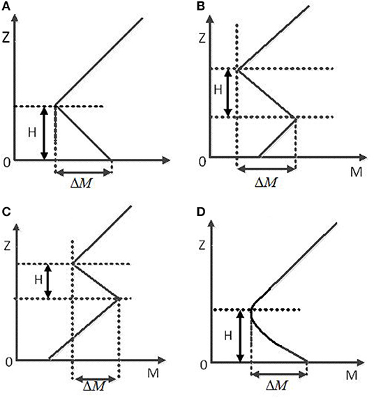
Figure 1. Atmospheric duct definitions: (A) surface duct; (B) surface-based duct; (C) elevated duct; (D) evaporation duct. (A–C) usually appears over land. The difference between (B) and (C) is that the atmospheric corrected refractivity M at the second inflection point of (B) is smaller than that at the ground, while (C) is larger than that at the ground. (D) usually appears over the ocean and its height h does not exceed 40 m.
Preprocessing of Atmospheric Duct Data
The meteorological data used in this paper are high-resolution radiosonde data from the global telecommunication system and inversion data from the DMSP satellite. The data location is an observation station in Hawaii (U.S. state), with longitude and latitude (155.1°W, 19.7°N). Data are taken daily at UTC = 12:00 from 2008 to 2009. The high-resolution sounding data include meteorological parameters such as temperature, pressure, humidity, and wind at the height of the sounding balloon. The vertical resolution is 10–80 m below 100 m and 30–300 m at 100–1,000 m, and the typical thicknesses of atmospheric ducts are between tens of meters and hundreds of meters, so these sounding data are appropriate for studying atmospheric ducts. The SST data from the DMSP satellite were provided by NOAA, with a spatial resolution of 0.25° × 0.25° and a temporal resolution of 3 h. The selected ocean area is about 1,000 m away from the station. First, the temperature, pressure, relative humidity, and wind speed at a height of 10 m are extracted from the high-resolution sounding data for each day. Then these data and the corresponding SSTs are put into the new height diagnostic model to diagnose the heights of evaporation ducts at this time. Finally, all calculation results are recorded as a time series X and the three points smoothing is then used to carry out low-pass filtering to get a new series X′. Specific methods are listed in section Preprocessing of Input Data. The series X′ obtained after smoothing is used for analysis and prediction by the traditional AR algorithm and the SVR algorithm improved by the simulated annealing operator. Considering the rapid change of the weather at sea, the influence of the ocean environment, measurement error, and turbulence, it is necessary to preprocess the meteorological data before using the new Liuli 2.0 model. Firstly, abnormal data are eliminated: specifically, the mean square deviation σ of the meteorological data is calculated, any data where the absolute difference between the data value and the average value is greater than 3σ are marked as an “abnormal value” and removed, and they are replaced using interpolation.
A New Diagnostic Model for Evaporation Duct Heights: The Liuli 2.0 Model
Introduction to the Liuli 2.0 Model
In the Liuli 2.0 model, the input parameters are atmospheric temperature, relative humidity, wind speed and pressure at a certain height, and SST. The height of the evaporation duct is obtained by introducing the K-theory flux observation method into the atmospheric refractive index equation. The difference between this model and the traditional model is that this model avoids the previous method of setting an initial value for the iterative calculation to determine the M-O length L and the characteristic parameters u∗, θ∗, and q∗, and instead selects a variable through the size of the overall Richardson number Rib, then uses the size of ξ to determine these characteristic parameters, which can improve the stability and efficiency of the calculation.
Flux Algorithm Calculation Scheme
At present, most flux calculation schemes need to be iterative and have low accuracy (Fairall et al., 2003). The non-iterative scheme adopted by the Liuli 2.0 model is similar to the classical iterative method. It uses multiple regression, which makes the calculation scheme applicable to a wide roughness range. The parameterization scheme depends on the atmospheric stratification. Under stable conditions, the scheme is divided into eight different categories according to the values of z/z0 and z/z0t, Where z0 is aerodynamic roughness length and z0t is thermodynamic roughness height (Li et al., 2014), as shown in Table 1.
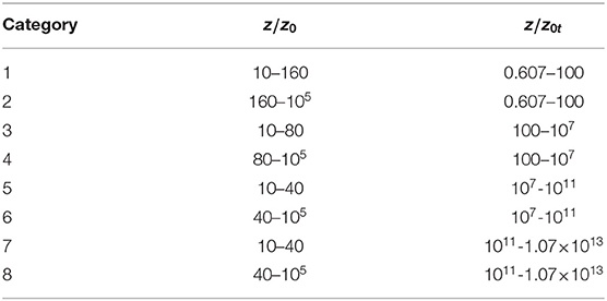
Table 1. The eight categories divided according to the values of z/z0 and z/z0t.
Then Ribcp is calculated according to the category corresponding to the values of z/z0 and z/z0t:
Values of Ribcp and Cmn for all categories are given in Li et al. (2014), and the parameters corresponding to the first category are shown in Table 2 as an example.

Table 2. The coefficients of Equation (4).
According to the value of Ribcp, we can determine the location of Rib: for example, when the size of Rib is between Ribcp1 and Ribcp2 it is section Introduction, when it is between Ribcp2 and Ribcp3 it is in section Atmospheric Duct Data, and so on. Finally, the following equation is used to calculate ξ:
The coefficients Cijk are given for the first category as an example, in Table 3.
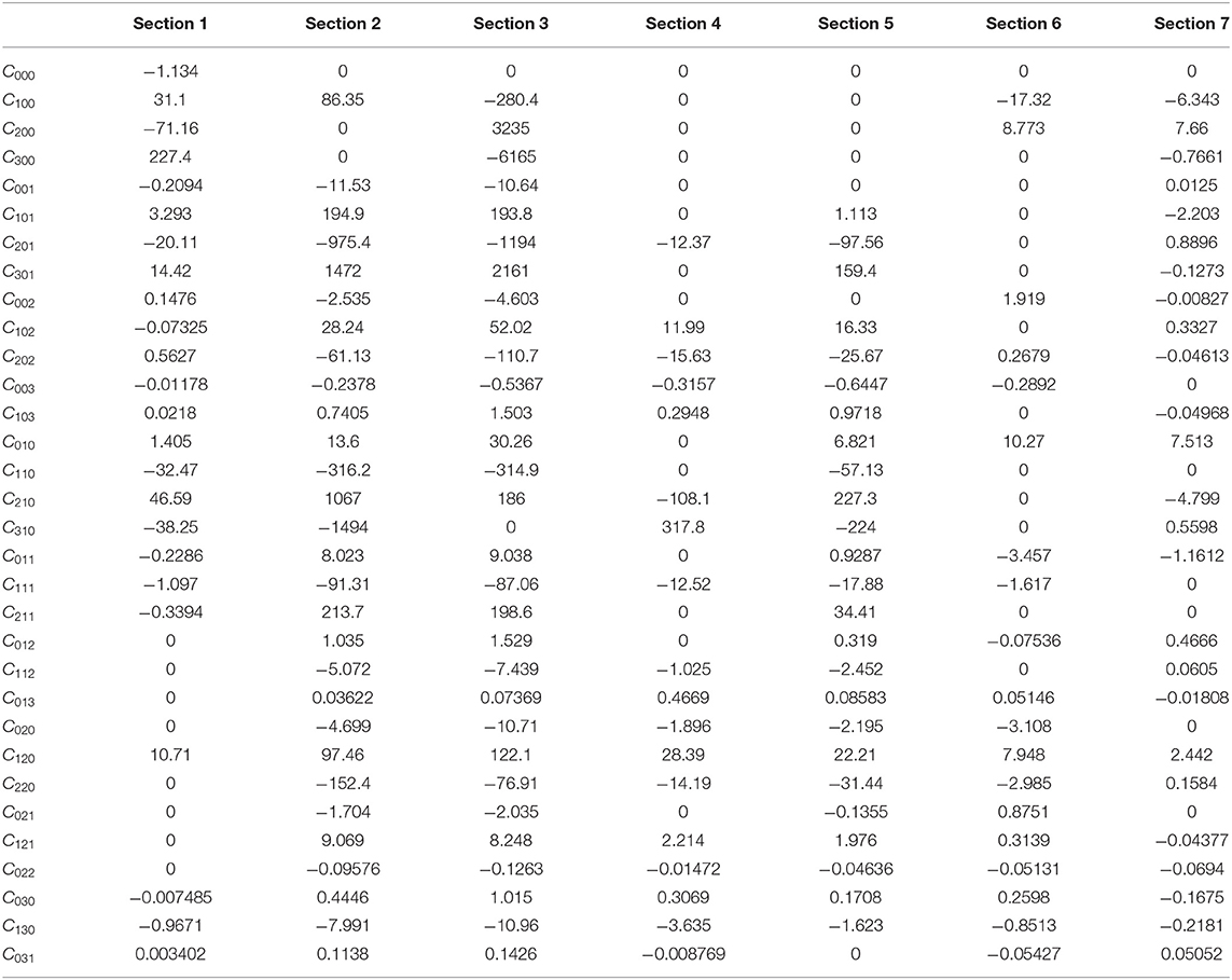
Table 3. Coefficients of Equation (6) for category 1.
Under unstable conditions, the scheme is divided into eight categories according to the values of Rib, z/z0, and z/z0t, as shown in Table 4.
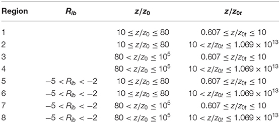
Table 4. The eight categories divided according to the values of Rib, z/z0 and z/z0t.
The value of ξ is calculated according to the category as follows:
The coefficients Cijk have different values according to the calculation results of different iteration schemes. This paper uses Cijk based on the results of the Paulson 70 scheme (Paulson, 1970), as shown in Table 5 for category 1.
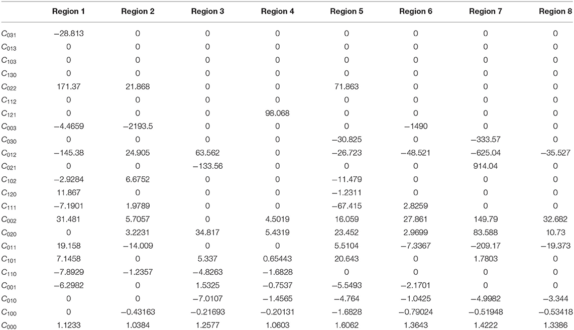
Table 5. Coefficients of Equation (8) for category 1.
In the flux algorithm scheme, the turbulent flux τ and sensible heat flux Hs are defined as:
Here, ρ is the air density, cp is the specific heat capacity at constant pressure, u∗ is the characteristic wind speed, and θ∗ is the characteristic temperature.
The overall transport coefficient of flux is defined as:
Here, κ is the von-Karman constant, z0 is the aerodynamic roughness height, z0t is the thermodynamic roughness, z0q is the water vapor roughness, and the coefficients λ = 1.5,μ = μm = 2.59, μ = μh = 0.95, and v = 0.5.
Under stable conditions, according to the CB05 flux scheme (Li et al., 2015), the stability correction function is defined as:
In Equation (14), a = 6.1, b = 2.5, c = 5.3, d = 1.1 and .
Under unstable conditions, the stability correction function is defined as:
In Equation (15), according to Paulson (1970), α = 16, Ah = 16, and Am = 16.
At the height of an evaporation duct, the following formula applies (Liu et al., 2017):
The following formula is used to determine φh and φq in this paper:
Under neutral conditions , the evaporation duct height is therefore given by:
under stable conditions, the evaporation duct height is given by:
and under unstable conditions, the evaporation duct height is given by:
Equations (18)–(20) can be used to calculate the heights of evaporation ducts under different atmospheric stratification conditions by selecting the appropriate iterative method.
Putting the meteorological data from the selected station into the model, the calculation results are shown in Figure 2. It can be seen from this that the evaporation duct heights form a stationary time series, which is roughly consistent with the height distribution of the evaporation ducts calculated by Babin et al. (1997) and Paulus (1985).
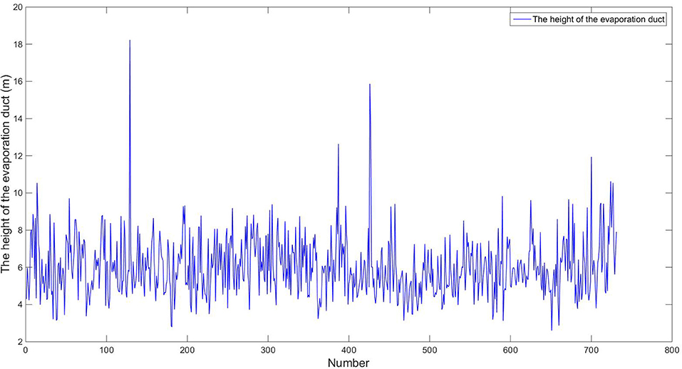
Figure 2. Evaporation duct heights diagnosed by the Liuli 2.0 model. The samples in the figure are from January 1, 2008 to December 31, 2019, which have 731 samples in total. Each sample in turn corresponds to the number 1–731 of the abscissa.
Prediction Method
Traditional AR Prediction Algorithm
Overview of AR
The auto-regressive (AR) algorithm is a time series processing method developed from linear regression analysis (Twiddle et al., 2006). The method uses itself as the regression variable, i.e., a linear combination of random variables in an earlier period is used to describe the linear regression process of random variables in a later period (Twiddle et al., 2006). Compared with other linear regression models, AR does not use x to predict y, but x to predict x. It is therefore widely used for prediction in economics, informatics, natural sciences, and other areas. Its basic principle is described in the following paragraph (see also Huang, 2004).
Suppose that a time series {Xt} satisfies:
where {at} is a white noise sequence and φ0, φ1, ···φp are real numbers. This algorithm is denoted as AR(p), and {Xt} suitable for this algorithm is called the sequence of AR(p). The centralized algorithm of AR is used in this paper, that is, φ0 = 0.
Generally, we can define the polynomial as the auto-regressive polynomial of an AR(p) algorithm.
Letting , the operator expression of the AR(p) algorithm can be expressed as:
From Equation (21), it can be concluded that:
so the solution of the AR(p) algorithm is as follows:
where ϕ0 = 1.
Establishment of the AR Algorithm
Preprocessing of input data
The evaporation duct height data calculated by the Liuli 2.0 model still contain a large amount of clutter, so it is necessary to carry out low-pass filtering to obtain a new sample sequence. The specific smoothing method is described in the following paragraph (see also Huang, 2004).
The 3-day smoothing average evaporation duct height is calculated on a 1-day time step as follows:
where is the average evaporation duct height calculated at the nth time, xi is the evaporation duct height value calculated at the ith time, and a is the first sample in the smoothing average range: when n ≤ N, a = 1, and when n > N, a = n−N+1; N is the total number of samples and n is the number of samples in the current smoothing average range. The result after smoothing is shown in Figure 3. The sample sequence X′obtained by smoothing is used for analysis and prediction by the traditional AR algorithm.
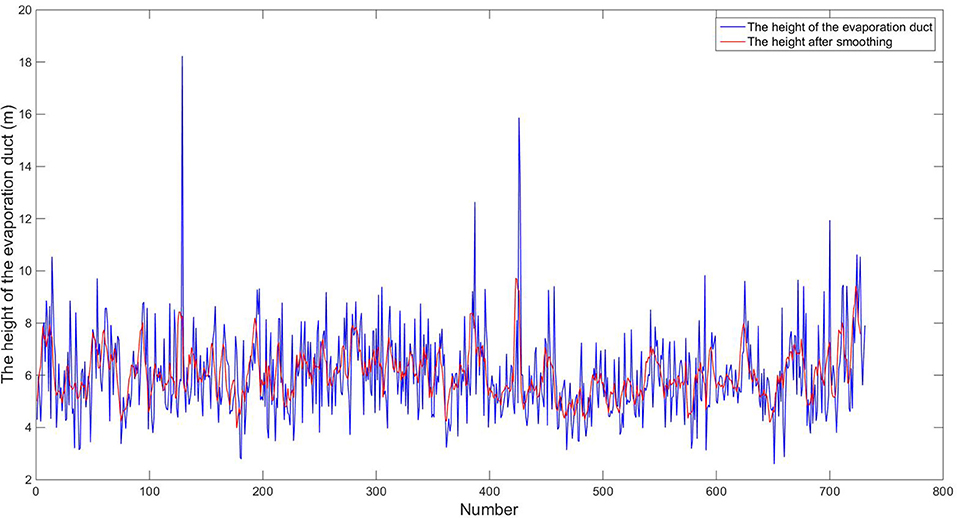
Figure 3. Original evaporation duct heights and heights after smoothing.
Choice of the order of the algorithm
In establishing an ideal algorithm AR(p), it is not possible to know in advance the appropriate order p. Different orders should be tested, so that the best order can be chosen for the final algorithm. Generally, the scheme used is a dynamic modeling scheme, which uses a series AR(m), (m = 1, 2…) to approximate data step by step, and, at each step, the approximation effect is evaluated by the reduction in the sum of squares of residuals. If the sum of squared residuals does not improve significantly, the test of further increasing m is not carried out. Experiment shows that if m is increased not by 1 but by 2 every time, this is advantageous, and more computationally efficient. The specific methods are described in the following (see also Huang, 2004).
If AR(m) is the current model, the AR(m+1) is the model to be tested. It is observed whether the reduction in the sum of the squares of the residuals exceeds a standard significance. This is carried out according to the following formula:
The variable F follows the F-distribution of the freedom degree of molecule s and denominator n-r. A0 is the sum of squares of residuals of the model to be tested, A1 is the sum of squares of the residuals of the previous model, r is the sum of two parameters of model A0, and s is the difference of a parameter between model A1 and model A0. In changing from AR(m) to AR(m + 1), if F > F5%, then the improvement in the sum of squares of the residuals is significant, implying that the AR(m) model is insufficient. If F < F5%, then AR(m) can be considered to be appropriate at this significance level. The results in Table 6 were obtained for this paper. It can be seen that, when m = 2, the model passes the 95% significance test. Therefore, in this paper, the AR(2) model is selected for the time series prediction.
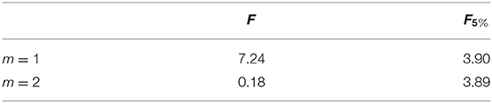
Table 6. Results of the F test.
The SVR Prediction Algorithm Improved by the Simulated Annealing Operator
Overview of the SVR
The support vector machine is an important part of statistical learning theory, and also the most practically applicable part (Yuan et al., 2010). In pattern recognition, in order to find decision rules with generalization ability, some subsets of the selected training data are denoted as support vectors. The best separation of support vectors is equivalent to the separation of all data. Support vector machines are similar to neural networks; the output is a linear combination of intermediate nodes, and each intermediate node corresponds to a support vector. Its structure is shown in Figure 4. In recent years, support vector machines have also shown excellent performance in research on regression algorithms, so a new algorithm has been developed, the support vector regression (Basak et al., 2007), which has been successfully applied to the prediction of time series.
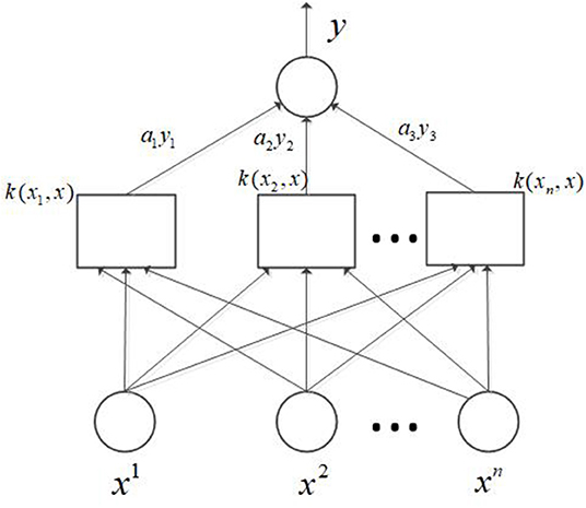
Figure 4. Structure of the support vector machine.
This paper uses the SVR, and the principle is described in the following (see also Basak et al., 2007):
For a given sample set , where the vector xi is the input sample of the model and yi is the corresponding output sample, the regression problem is to find out the relationship between xi and yi:
Here, < · > represents a mapping of the input samples in the original space to the inner product of the high-dimensional space using the kernel function, so that the non-linear problem in the original space can be transformed into a linear problem in the high-dimensional space. The insensitivity loss ε(ε > 0) is introduced, according to:
When the loss function satisfies this equation, the optimal solution is obtained. By introducing relaxation variables of ξi and , the above problems can be transformed into optimization problems as follows:
Here, the first term improves the generalization ability, and the second item improves the accuracy. To solve these optimization problems, a Lagrangian function is constructed:
where .
In Equation (30), the partial derivatives with respect to w, b, ξi, and are calculated as follows:
After simplifying Equation (31), we obtain:
In Equation (32), sample data for which is not equal to zero represent the support vector. The dual form of the non-linear optimization problem can be obtained from Equation (32), so the regression function can be rewritten as:
Therefore, using existing input and output samples, the output expression is obtained through the training of the SVR, and then, using Equation (33), the output data of a new sample can be obtained by inputting data from this sample, so as to achieve the data prediction.
Establishment of the Improved SVR Algorithm
Preprocessing of input data
Similarly to the auto-regressive algorithm, the improved SVR algorithm needs to preprocess the data before they are input. The method is the same as for the auto-regressive algorithm, so it will not be repeated here.
Normalization of data
In order to prevent output saturation caused by large absolute input values, the training sample is normalized before it is input to the input layer of the SVR, so that the data vector falls within the range [0,1] or [−1,1]; it also needs to be denormalized when the SVR outputs the data. The normalization means that input and output vector data have similar weights in each dimension and prevents one dimension from dominating the weighting algorithm. The normalization formula is as follows:
where xi is the input or output data, xmin is the minimum value in the dataset, and xmax is the maximum value in the dataset.
Selection of algorithm parameters
The selection process for the improved SVR algorithm includes the choice of kernel function and the optimization of parameters.
Selection of kernel function. There are mainly three kinds of kernel functions: linear kernel function, polynomial kernel function, and radial basis kernel function. The linear kernel function is not suitable for this algorithm, because the SVR is non-linear. The polynomial kernel function has many super-parameters, which makes its structure complex. In addition, polynomial kernel function is suitable for orthogonal normalized data, so it is also not suitable for this algorithm. The radial basis function (RBF) kernel is a kind of kernel function with strong locality, which can map a sample to a higher dimensional space for both large and small samples, and it has better anti-interference ability for the noise in the data. Besides, it has only one super-parameter σ, so this is chosen for this paper. The expression is as follows:
Selection of parameters. The main parameters to be selected in the prediction model are the penalty parameter C, the insensitivity loss degree ε, and kernel function parameter σ. To select these three parameters, we use the simulated annealing operator (Serrurier and Prade, 2008) to find the optimal values. The simulated annealing operator starts from a certain state and adjusts the current state according to the current temperature to generate a new state (Serrurier and Prade, 2008). It has five adjustable parameters: the starting temperature T (T = 1 × 10⁷), the ending temperature Tmin (Tmin = 1 × 10⁻⁶), temperature decreasing rate C1 (C1 = 0.99), the maximum number of iterations N (N = 1 × 10⁸), and the minimum boundary value of each parameter n (n = 1 × 10⁻⁸). If the new state is better, the new state is accepted. If the new state is worse, a probability will be generated based on the current temperature and the difference between the results of the two states. The system then decides whether to accept the state according to this probability. After each state transition, the temperature value is reduced, and the search stops the temperature value goes below a predetermined minimum value.
In this paper, the state is determined by three variables, the penalty parameter C, insensitivity loss ε, and kernel function parameter σ. The vector Xi composed of these three variables is taken as a state, and the RMSE of the regression prediction algorithm obtained for this state is taken as the evaluation function f(Xi). The specific steps are illustrated in Figure 5, and are described as follows:
(1) Set the initial state Xi, temperature T and minimum temperature Tmin
(2) Move to the next state based on the current state
(3) If f(Xi) > , accept the status and go to (5)
(4) Generate the probability , and generate a random number p between 0 and 1. If p < P, the system accepts the state, otherwise it does not.
(5) Calculate T= T * 0.99, if the current value of f(X′) is the optimal value, the new optimal state is retained.
(6) If T < Tmin, the algorithm ends, otherwise go to (2).
After applying the above algorithm, the optimal parameters found were: C=187511.19, ε=0.00181, and σ=0.001812.
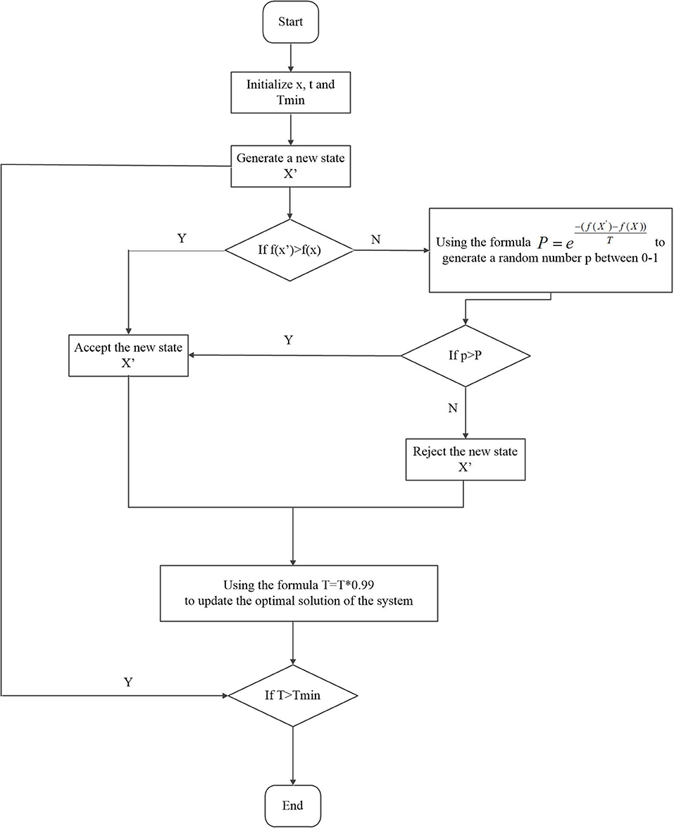
Figure 5. Flow chart of the improved SVR.
Discussion and Analysis of Results
The total number of sample X′ is 731, after the algorithm is completed, the first 549 samples are used as training sets, and the last 182 samples are used as test sets to verify whether the predicted results are similar to the actual values. Figures 6–8 show comparisons between predicted values using the three algorithms, and real values, for the last 182 samples of time series X′.
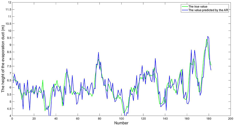
Figure 6. Real values and values predicted by AR algorithm. The samples in the figure are from July 3, 2008 to December 31, 2019, which have 182 samples in total. Each sample in turn corresponds to the number 1–182 of the abscissa.
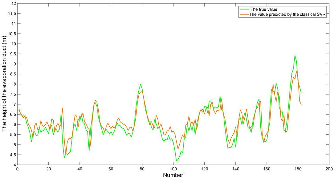
Figure 7. Real values and values predicted by classical SVR algorithm. The samples in the figure are from July 3, 2008 to December 31, 2019, which have 182 samples in total. Each sample in turn corresponds to the number 1–182 of the abscissa.
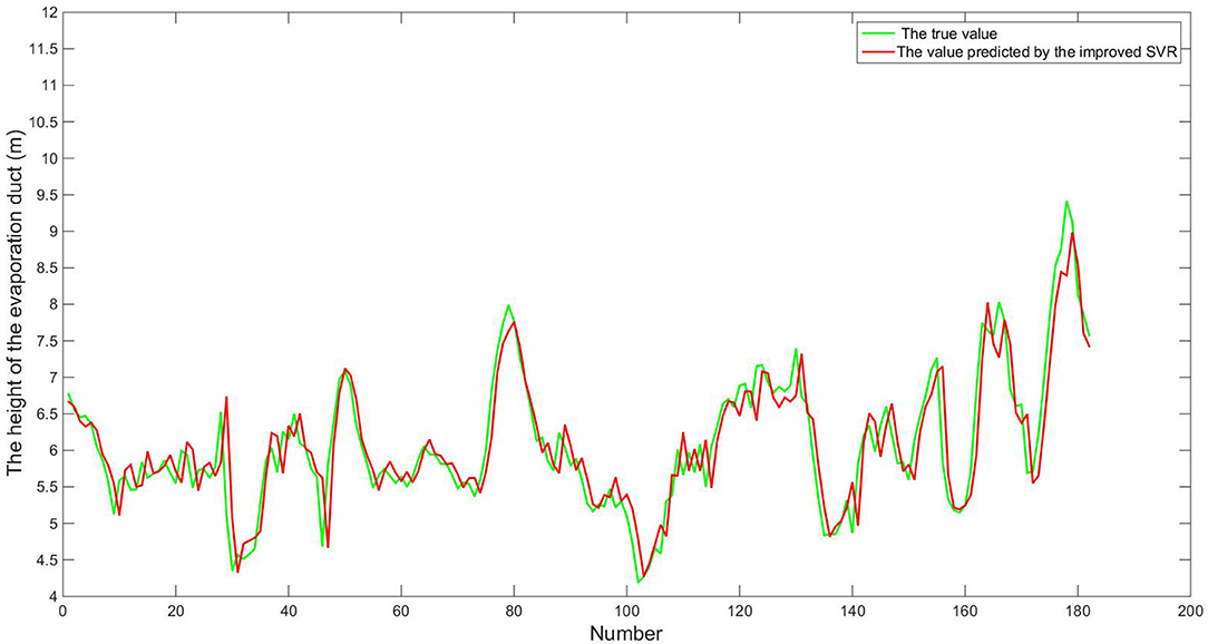
Figure 8. Real values and values predicted by improved SVR algorithm. The samples in the figure are from July 3, 2008 to December 31, 2019, which have 182 samples in total. Each sample in turn corresponds to the number 1–182 of the abscissa.
From Figures 6–8, we can see that the prediction curves of the three algorithms follow the same trends as the true values. In order to evaluate the quality of prediction, we use RMSE and MAPE, which are calculated as follows:
Figures 9, 10 show the individual RMSEs and MAPEs of the last quarter of time series X′, using the three prediction algorithms. Table 7 shows the corresponding overall RMSE and MAPE values.
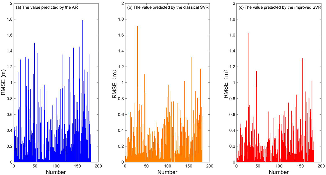
Figure 9. RMSE of evaporation duct heights.
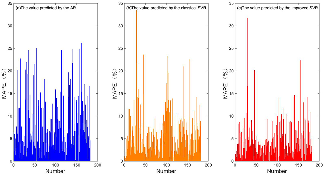
Figure 10. MAPE of evaporation duct heights.
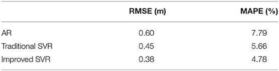
Table 7. Analysis of overall error.
From Figures 9, 10, we can see that nearly one-third of the RMSE values using the traditional AR algorithm are more than 0.5, and nearly one-third of the MAPE values are more than 10%, and nearly one-fourth of the RMSE values using the classical SVR algorithm are more than 0.5, and nearly one-fourth of the MAPE values are more than 10%, whereas most of the RMSE values using the improved SVR algorithm are less than 0.5, and most of the MAPE values are less than 10%. From Table 7, we can see that the overall RMSE using the traditional AR algorithm is 0.60, and the MAPE is 7.79%, and the overall RMSE using the classical SVR algorithm is 0.45, and the MAPE is 6.10%, while the overall RMSE using the improved SVR algorithm is 0.38, and the MAPE is 4.78%. The prediction error of improved SVR algorithm is about 37% lower than that of the traditional AR algorithm and 15% lower than that of the classical SVR algorithm. Figures 11–13 are the fitting graphs obtained by univariate linear regression (Neto et al., 2004) of the real and predicted values of the last 182 samples of the time series.
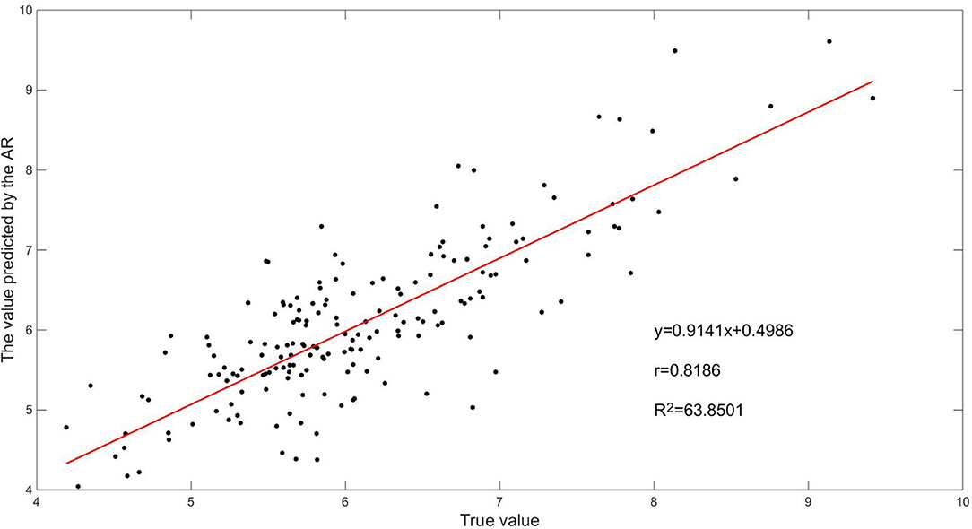
Figure 11. Fitting graph for the result of AR algorithm.
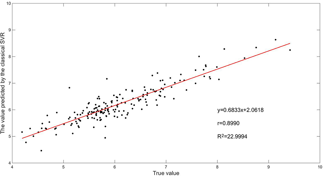
Figure 12. Fitting graph for the result of classical SVR algorithm.
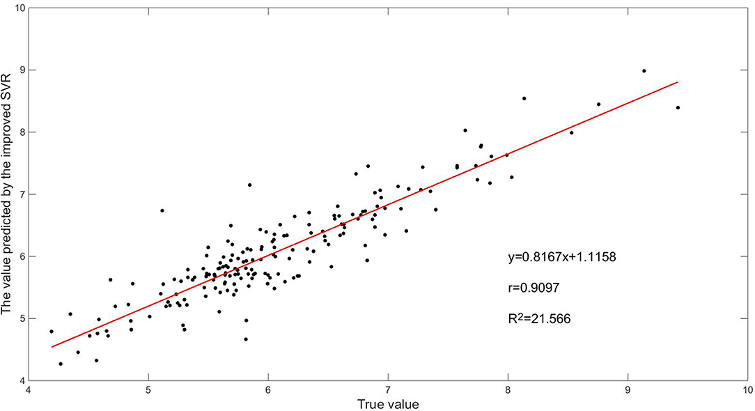
Figure 13. Fitting graph for the result of improved SVR algorithm.
From Figures 11–13, we can see that the correlation coefficient r of the traditional AR algorithm is 0.8186, and the sum of squares of residuals is R2 = 63.8501, and the correlation coefficient r of the classical algorithm is 0.8990, and the sum of squares of residuals is R2 = 22.9994, while the correlation coefficient r of the improved SVR algorithm is 0.9097, and the sum of squares of residuals is R2 = 21.566. The prediction accuracy of the improved SVR algorithm is the highest, so its correlation coefficient r is the largest, and its residual adjustment and R2 is the smallest, which shows that it has a better performance overall.
Conclusion and Future Work
In this paper, a new diagnostic model of evaporation duct heights, the Liuli 2.0 model, is proposed. The difference between this model and the traditional model is that, when determining the M-O length L and the characteristic parameters u∗,θ∗, and q∗, it avoids the previous method of setting an initial value for an iterative calculation to determine these parameters, but instead selects a variable , through the size of the overall Richardson number Rib, then uses the size of ξ to determine the characteristic parameters. This can improve the stability and efficiency of the calculation, saving a large amount of computation time. Using high-resolution sounding data and retrieved SST data from the DMSP satellite from 2008 to 2009 at a Hawaiian station, the height of the evaporation ducts near the station is diagnosed according to the model. Then, the traditional AR algorithm, classical SVR algorithm and the SVR algorithm improved by a simulated annealing operator, are used to analyze and predict time series of evaporation duct heights, and the prediction results are compared to verify the advantages and disadvantages of the improved SVR algorithm. The results show that the prediction error of the improved SVR algorithm is 37% lower than that of the traditional AR algorithm and 15% lower than that of the classical SVR algorithm. It has a good accuracy and strong generalization ability, and acts as a reference for the study of short-term prediction of evaporation duct heights. The new diagnosis and prediction method will provide a new method for studying the evaporation duct heights, which has certain reference significance for the study of the evaporation ducts.
However, evaporation duct heights have a significant seasonal variation, which is not discussed in this paper. Therefore, future work will be applied to predicting the seasonal characteristics of evaporation ducts. In addition, when predicting, the regression function expression f(x) obtained by the improved SVR algorithm is fixed and not updated with new observation data, that is, f(x) is “static.” In future work, a “dynamic” f(x) will be introduced, to enhance the prediction model of atmospheric ducts using the real-time observation data, so as to further improve the accuracy of the predictions.
Data Availability Statement
The high-resolution sounding data from the global positioning system are provided at https://www.sparc-climate.org. The SST data are available from www.ncc-cma.net.
Author Contributions
ZS, YM, and CL design the improved SVR algorithm. LL provided the new diagnostic model of evaporation duct heights. All authors have contributed to the interpretation of the results and the preparation of the manuscript. All authors read and approved the final manuscript.
Funding
This study was partly supported by the National Natural Science Foundation of China (Grant no. 41875045 and 41775039).
Conflict of Interest
The authors declare that the research was conducted in the absence of any commercial or financial relationships that could be construed as a potential conflict of interest.
Acknowledgments
Thanks to Stratosphere-troposphere Processes and their Role in Climate (SPARC) and the National Oceanic and Atmospheric Administration (NOAA) for providing data used in this study.
References
Babin, S. M., and Dockery, G. D. (2002). LKB-based evaporation duct model comparison with buoy data. J. Appl. Meteorol. 41, 434–446. doi: 10.1175/1520-0450(2002)041<0434:Lbedmc>2.0.Co;2
Babin, S. M., Young, G. S., and Carton, J. A. (1997). A new model of the oceanic evaporation duct. J. Appl. Meteorol. 36, 193–204. doi: 10.1175/1520-0450(1997)036<0193:ANMOTO>2.0.CO;2
Bankert, R. L., Hadjimichael, M., Kuciauskas, A. P., Richardson, K. L., Turk, J., Hawkins, J. D., et al. (2002). “Automating the estimation of various meteorological parameters using satellite data and machine learning techniques,” in Igarss 2002: IEEE International Geoscience and Remote Sensing Symposium and 24th Canadian Symposium on Remote Sensing, Vols. I–VI, Proceedings: Remote Sensing: Integrating Our View of the Planet (Toronto. ON).
Basak, D., Srimanta, P., and Patranbis, D. C. (2007). Support vector regression. Neural Inform. Process. Lett. Rev. 11, 203−224. doi: 10.1007/978-1-4302-5990-9_4
Burk, S. D., Haack, T., Rogers, L. T., and Wagner, L. J. (2003). Island wake dynamics and wake influence on the evaporation duct and radar propagation. J. Appl. Meteorol. 42, 349–367. doi: 10.1175/1520-0450(2003)042<0349:IWDAWI>2.0.CO;2
Chang, S., Sheng, Z., Du, H., Ge, W., and Zhang, W. (2020). A channel selection method for hyperspectral atmospheric infrared sounders based on layering. Atmos. Meas. Tech. 13, 629–644. doi: 10.5194/amt-13-629-2020
Czernecki, B., Nowosad, J., and Jablonska, K. (2018). Machine learning modeling of plant phenology based on coupling satellite and gridded meteorological dataset. Int. J. Biometeorol. 62, 1297–1309. doi: 10.1007/s00484-018-1534-2
Ebtehaj, I., and Bonakdari, H. (2016). A support vector regression-firefly algorithm-based model for limiting velocity prediction in sewer pipes. Water Sci. Technol. 73, 2244–2250. doi: 10.2166/wst.2016.064
Fairall, C. W., Bradley, E. F., Hare, J. E., Grachev, A. A., and Edson, J. B. (2003). Bulk parameterization of air-sea fluxes: Updates and verification for the COARE algorithm. J. Clim. 16, 571–591. doi: 10.1175/1520-0442(2003)016<0571:Bpoasf>2.0.Co;2
Ham, Y.-G., Kim, J.-H., and Luo, J.-J. (2019). Deep learning for multi-year ENSO forecasts. Nature 573, 568–572. doi: 10.1038/s41586-019-1559-7
He, X., Guo, J., Wu, J., Li, X., Tian, B., Zhong, Y., et al. (2018). Short-term forecast for evaporation duct height based on time series. J. Electron. Meas. Instrum. 32, 102–103. doi: 10.13382/j.jemi.2018.01.014
He, Y., Sheng, Z., and He, M. (2020). Spectral analysis of gravity waves from near space high-resolution balloon data in Northwest China. Atmosphere 11:133. doi: 10.3390/atmos11020133
Huang, J. (2004). “The analysis of time series,” in The Meteorological Statistical Analysis and Forecast Method, 3rd Edn, ed R. Zhang (Beijing: Meteorology Press), 195–198.
Ivanov, V. K., Shalyapin, V. N., and Levadnyi, Y. V. (2007). Determination of the evaporation duct height from standard meteorological data. Izvestiya Atmos. Ocean. Phys. 43, 36–44. doi: 10.1134/s0001433807010045
Kang, S., Zhang, Y., and Wang, H. (2014). “The characteristics and detection of atmospheric duct,” in Atmospheric Ducts in the Troposphere, 3rd Edn, ed Z. Wang (Beijing: Science Press), 44–53.
Lee, M.-K., Moon, S.-H., Kim, Y.-H., and Moon, B.-R. (2014). “Correcting abnormalities in meteorological data by machine learning,” in: 2014 IEEE International Conference on Systems, Man and Cybernetics. IEEE International Conference on Systems Man and Cybernetics Conference Proceedings (San Diego, CA: IEEE), 888–893.
Li, Y., Gao, Z., Li, D., Chen, F., Yang, Y., and Sun, L. (2015). An update of non-iterative solutions for surface fluxes under unstable conditions. Bound. Layer Meteorol. 156, 501–511. doi: 10.1007/s10546-015-0032-x
Li, Y., Gao, Z., Li, D., Wang, L., and Wang, H. (2014). An improved non-iterative surface layer flux scheme for atmospheric stable stratification conditions. Geosci. Model Dev. 7, 515–529. doi: 10.5194/gmd-7-515-2014
Liu, C., Huang, J., and Jiang, C. (2001). Modeling evaporation duct over sea with pseudo-refractivity and similarity theory. Acta. Electronica. Sinica. 29, 107–109. doi: 10.3321/j.issn:0372-2112.2001.07.030
Liu, L., Li, Y., Gao, Z., Bi, X., and Chen, Q. (2017). The prediction model of evaporation duct based on non iterative sea air flux algorithm. J. Appl. Oceanogr. 36, 23–25.
Liu, L., Li, Y., Gao, Z., Bi, X., and Zhu, G. (2019). Comparison and analysis of four kinds of evaporation duct model. J. Meteorol. Sci. 39, 82–96. doi: 10.3969/2017jms.0037
Mai, Y., Sheng, Z., Shi, H., Liao, Q., and Zhang, W. (2020). Spatiotemporal distribution of atmospheric ducts in Alaska and its relationship with the Arctic vortex. Int. J. Antennas Propag. 2020, 1–13. doi: 10.1155/2020/9673289
Neto, E. D., de Carvalho, F. A. T., and Tenorio, C. P. (2004). “Univariate and multivariate linear regression methods to predict interval-valued features,” in Ai 2004: Advances in Artificial Intelligence,in Proceedings, Vol. 3339, eds G. I. Webb and X. Yu (Cairns), 526–537. https://doi.org/10.1007/978-3-540-30549-1_46
Paulson, C. A. (1970). The mathematical representation of wind speed and temperature profiles in the unstable atmospheric surface layer. Appl. Meteorol. 9, 857–861. doi: 10.1175/1520-0450(1970)009<0857:TMROWS>2.0.CO;2
Paulus, R. A. (1985). Practical application of an evaporation duct model. Radio Sci. 20, 887–896. doi: 10.1029/RS020i004p00887
Rhee, J., and Im, J. (2017). Meteorological drought forecasting for ungauged areas based on machine learning: using long-range climate forecast and remote sensing data. Agric. For. Meteorol. 237, 105–122. doi: 10.1016/j.agrformet.2017.02.011
Serrurier, M., and Prade, H. (2008). Improving inductive logic programming by using simulated annealing. Inform. Sci. 178, 1423–1441. doi: 10.1016/j.ins.2007.10.015
Sheng, Z., and Huang, S.-X. (2009). Ocean duct inversion using radar clutter and its noise restraining ability. Acta Phys. Sin. 58, 4328–4334. doi: 10.1360/972008-2465
Sheng, Z., and Huang, S.-X. (2010). Ocean duct inversion from radar clutter using variation adjoint and regularization method (II): inversion experiment. Acta Phys. Sin. 59, 3912–3916. doi: 10.7498/aps.59.3912
Shi, Y., Zhang, Q., Wang, S., Yang, K., Yang, Y., Yan, X., et al. (2019). A comprehensive study on maximum wavelength of electromagnetic propagation in different evaporation ducts. IEEE Access 7, 82308–82319. doi: 10.1109/access.2019.2923039
Tag, P. M., and Peak, J. E. (1996). Machine learning of maritime fog forecast rules. J. Appl. Meteorol. 35, 714–724. doi: 10.1175/1520-0450(1996)0352.0.CO;2
Tian, B., Cha, H., and Zhang, Y. (2009a). Study on the applicability of evaporation duct model A in Chinese sea areas. Chinese J. Radio Sci. 24, 176–181.
Tian, B., Yu, S., Li, J., and Jiang, H. (2009b). Study on the applicability of PJ evaporation duct model in semitropical sea areas. Ship Sci. Technol. 31, 99–102.
Twiddle, J. A., Spurgeon, S. K., Kitsos, C., Jones, N. B., and Ieee (2006). “A discrete-time Sliding Mode Observer for estimation of auto-regressive model coefficients with an application in condition monitoring,” in 2006 International Workshop on Variable Structure Systems (Alghero).
Wang, W., Guan, M., Tian, W., Schmidt, T., and Ding, A. (2019). Large uncertainties in estimation of tropical tropopause temperature variabilities due to model vertical resolution. Geophys. Res. Lett. 46, 10043–10052. doi: 10.1029/2019GL084112
Wang, Y., Wu, D. L., Guo, C. X., Wu, Q. H., Qian, W. Z., and Yang, J. (2010). “Short-term wind speed prediction using support vector regression,” in IEEE Power and Energy Society General Meeting 2010. IEEE Power and Energy Society General Meeting PESGM (Providence, RI).
Xie, F., Li, J., Zhang, J., Tian, W., Hu, Y., Zhao, S., et al. (2017). Variations in north Pacific sea surface temperature caused by Arctic stratospheric ozone anomalies. Environ. Res. Lett. 12:114023. doi: 10.1088/1748-9326/aa9005
Xue, S., Yang, M., Li, C., et al. (2009). “Meteorological prediction using support vector regression with genetic algorithms[C],” in International Conference on Information Science and Engineering (Nanjing: IEEE). doi: 10.1109/ICISE.2009.735
Yang, S., Li, X., and Wu, J. (2016). Adaptability research of evaporation duct predication model based on NPS model. J. Electron. Meas. Instrum. 30, 1899–1906. doi: 10.13382/j.jemi.2016.12.013
Yu, G., Liu, A., and Yang, Y. (2015). Babin model of evaporation waveguide diagnosis and its sensitivity analysis. J. Astron. Metrol. Meas. 35, 53–56. doi: 10.3969/j.issn.1000-7202.2015.02.015
Yuan, F., Kumar, U., and Galar, D. (2010). Reliability prediction using support vector regression. Int. J. Syst. Assur. Eng. Manage. 1, 263–268. doi: 10.1007/s13198-011-0040-2
Zhang, J., Tian, W., Chipperfield, M., Xie, F., and Huang, J. (2016). Persistent shift of the Arctic polar vortex towards the Eurasian continent in recent decades. Nat. Clim. Change 6, 1094–1099. doi: 10.1038/nclimate3136
Keywords: evaporation duct heights, new diagnostic height model, AR algorithm, improved SVR algorithm, time series
Citation: Mai Y, Sheng Z, Shi H, Li C, Liu L, Liao Q, Zhang W and Zhou S (2020) A New Diagnostic Model and Improved Prediction Algorithm for the Heights of Evaporation Ducts. Front. Earth Sci. 8:102. doi: 10.3389/feart.2020.00102
Received: 15 December 2019; Accepted: 23 March 2020;
Published: 17 April 2020.
Edited by:
Jing-Jia Luo, Bureau of Meteorology, AustraliaReviewed by:
Isa Ebtehaj, Razi University, IranFei Xie, Beijing Normal University, China
Wuke Wang, China University of Geosciences Wuhan, China
Copyright © 2020 Mai, Sheng, Shi, Li, Liu, Liao, Zhang and Zhou. This is an open-access article distributed under the terms of the Creative Commons Attribution License (CC BY). The use, distribution or reproduction in other forums is permitted, provided the original author(s) and the copyright owner(s) are credited and that the original publication in this journal is cited, in accordance with accepted academic practice. No use, distribution or reproduction is permitted which does not comply with these terms.
*Correspondence: Zheng Sheng, 19994035@sina.com