 Zhicong Yan
 Shenghong Li1*
- 1Department of Cyber Science and Engineering, Shanghai Jiao Tong University, Shanghai, China
- 2School of Art and Design, Zhengzhou Institute of Industrial Application Technology, Zhengzhou University, Zhengzhou, Hebei, China
- 3School of Information Science and Engineering, Hangzhou Normal University, Hangzhou, Zhejiang, China
Semi-supervised learning (SSL) methods provide a powerful tool for utilizing abundant unlabeled data to strengthen standard supervised learning. Traditional graph-based SSL methods prevail in classical SSL problems for their intuitional implementation and effective performance. However, they encounter troubles when applying to image classification followed by modern deep learning, since the diffusion algorithms face the curse of dimensionality. In this study, we propose a simple and efficient SSL method, combining a graph-based SSL paradigm with differential privacy. We aim at developing coherent latent feature space of deep neural networks so that the diffusion algorithm in the latent space can give more precise predictions for unlabeled data. Our approach achieves state-of-the-art performance on the Cifar10, Cifar100, and Mini-imagenet benchmark datasets and obtains an error rate of 18.56% on Cifar10 using only 1% of all labels. Furthermore, our approach inherits the benefits of graph-based SSL methods with a simple training process and can be easily combined with any network architecture.
1. Introduction
Deep neural networks (DNN) have become the first choice for computer vision applications due to their prominent performance and flexibility. However, the harsh requirement for precisely annotated data has largely constrained the wide application of deep learning. It is generally known that the collection and annotation of large-scale data are extremely costly and time-consuming in some professional industries (e.g., healthcare, finance, and manufacturing). Therefore, semi-supervised learning (SSL), which utilizes abundant unlabeled data in deep learning applications, has become an important research trend in the field of artificial intelligence (Chapelle et al., 2006; Tarvainen and Valpola, 2017; Iscen et al., 2019).
Various approaches to SSL in terms of image classification have been proposed in recent years based on some prototypical assumptions. For instance, the manifold assumption, which states that high dimensional data usually lie on low dimensional manifolds, leads to some consistency-based SSL methods. Other two well-known assumptions, cluster assumption, and low-density separation assumption have also inspired some types of research. To summarize, two main research directions show great promise.
One direction explores generative model-based approaches. For instance, VAE (Kingma and Welling, 2013), generative adversarial network (GAN) (Goodfellow et al., 2014), and normalizing flows (Kobyzev et al., 2020) can establish a low-dimensional hidden variable capturing the manifold of the input data, and then, Bayesian inference can be applied to optimize the posterior probability of both labeled and unlabeled examples (Kingma et al., 2014; Makhzani et al., 2015; Rasmus et al., 2015; Maaløe et al., 2016). However, GAN is known to be extremely difficult in generating high-resolution images, despite a large amount of research in recent years (Radford et al., 2015; Gulrajani et al., 2017; Brock et al., 2018), making these approaches difficult to scale to large and complex dataset (Yu et al., 2019). Furthermore, the extensive computation cost in training generative models makes these approaches less practical in real-world applications (Brock et al., 2018).
Another direction tries to exert proper regularizations on the classifier using unlabeled data. Those regularizations could be summarized into two categories as follows: one is consistency regularization, where two similar images or two networks with related parameters are encouraged to have similar network outputs (Sajjadi et al., 2016; Tarvainen and Valpola, 2017; Miyato et al., 2019). Another type is based on the data graph. In traditional machine learning, manifold assumption-based algorithms usually establish a graph to describe the manifold structure, then employ the graph Laplacian to induce smoothness on the data manifold, such as Harmonic function (HF) (Zhu et al., 2003), Label Propagation (LP) (Zhou et al., 2003; Gong et al., 2015), and Manifold Regularization (MR) (Belkin et al., 2006).
Those two types of semi-supervised methods have their strengths and weakness, respectively. In terms of consistency-based regularization, those methods only consider the perturbations around each data point, ignoring the connections between data points. Therefore, they do not fully utilize the data structure, such as manifolds or clusters. This artifact could be avoided if the data structure is taken into consideration using graph-based methods, which define convex optimization problems and have closed form of solutions (Zhou et al., 2003; Gong et al., 2015; Tu et al., 2015). On the contrary, the performance of the graph-based methods will degrade if the input data graph cannot satisfy the following conditions (Belkin et al., 2006): capturing the manifold structure of the input space and representing the similarity between two data points. Some traditional research aims at improving the graph quality (Jebara et al., 2009). However, it is extremely difficult to capture the manifold of high-dimensional image data, causing poor performance on image recognition tasks (Kamnitsas et al., 2018; Luo et al., 2018; Li et al., 2020, 2022; Ren et al., 2022).
Motivated by the above observation, we introduce differential privacy (Dwork and Roth, 2014) and mixup data augmentation (Zhang et al., 2018) in the graph-based SSL method. For both labeled and unlabeled data points, we force the predictions of network changes linearly in the vector from one data point to another, which forces the middle features to change linearly as well. We also employ differential privacy, to further boost the consistency of latent feature space by adding random noise to its latent representation layers. We observe that such regularization results in a more compact and coherent latent feature space given by the network and leads to a high-quality graph that captures the data manifold more accurately. Compared with the consistency-based methods (Sajjadi et al., 2016; Tarvainen and Valpola, 2017; Miyato et al., 2019), the proposed method demonstrate dominant performance with fewer label and much higher convergence speed, which means it can achieve the same performance with fewer computational cost. Compared with previous graph-based SSL methods, the proposed method tends to form more coherent latent feature space and achieves higher performance.
To summarize, there are two key contributions of our study as follows:
• We propose a simple but effective regularization method that can be applied to a graph-based SSL framework to regularize the latent space of deep neural network during the training process so that the graph-based SSL framework can work better with high-dimensional image datasets.
• We experimentally show that the proposed method achieves significant performance in improvement over the previous graph-based SSL method (Iscen et al., 2019) on SSL standard benchmarks and demonstrates competitive results to other state-of-the-art SSL methods.
2. Related work
In this section, we roughly categorized the recent advances in SSL into generative methods and graph-based methods and briefly introduce these two types of methods.
2.1. Generative SSL methods
Instead of directly estimating posterior probability p(y|x), the generative methods pay attention to learning the class distributions P(x|y) or the joint distribution p(x, y) = p(x|y)p(y), to compute the posterior probability using Bayes' formula. In this framework, SSL can be modeled as a missing data problem while the unlabeled data can be used to optimize the marginal distribution . The joint log-likelihood on both labeled data set DL and unlabeled data set DU is naturally considered an objective function (Chapelle et al., 2006) as follows:
where πy = p(y|θ) is class prior. Previous studies under this framework use auto-encoder (Rasmus et al., 2015) or variational auto-encoder (Kingma and Welling, 2013) to model p(x, y). Unfortunately, since the neural network has excessive representational power, optimizing marginal distribution cannot guarantee to achieve the right joint distribution, making those approaches perform less well in large datasets.
To better estimate p(x|y), generative adversarial network (GAN) (Goodfellow et al., 2014) has been introduced to the SSL framework. GAN is well-known for high-quality realistic image generation, Radford et al. (2015) employed fake examples from a conditional GAN as additional training data. Salimans et al. (2016) strengthened the discriminator to classify input data as well as distinguish fake examples from real data. Besides, BadGAN (Dai et al., 2017) argued that generating low-quality examples which lie in low-density areas between different classes can better guide the classifier position its the decision boundary. However, those approaches are based on practice and lack theoretical analysis, showing weak performance compared with newly emerged approaches.
2.2. Graph-based SSL methods
Graph-based methods operate on a weighted graph G = (V, E) with adjacency matrix A, where the vertex set V is composed of all data samples denoted as D = DL ∪ DU, and the elements of adjacency matrix Aij are based on similarities between vertices xi, xj ∈ V. The smoothness assumption states that close data points should have similar predictions. Label Propagation (LP) iteratively propagated the class posterior of each node to its neighbors, faster through a short connection between data nodes, until a global equilibrium is reached. Zhou et al. (2003) showed that the same solution is arrived at by enforcing the smoothness term or equivalently minimizing the energy on the graph as follows:
Here, fi is the pseudo label of the i-th data sample, Δ = D − A is the traditional graph Laplacian where D is a diagonal matrix with . If f is replaced with f(X) which is the output of a parameterized function on all data samples, the R(f) reaches a graph Laplacian regularizer which forces the function f to be harmonic. Some modifications to Equation (2) are made to mitigate the effect of outliers in the graph (Gong et al., 2015; Tu et al., 2015). An inevitable drawback of these approaches is that their performance largely relies on the quality of the input graph.
Our study is inspired by a series of recent methods which utilize the LP with a dynamically constructed graph in the optimization process. Acting like EM algorithms, those methods alternate between the two steps, the first step is to use the embeddings obtained by the deep neural network to construct the nearest neighbor graph, and then LP is performed on this graph to infer pseudo-label for the unlabeled images. After that, the network is trained using both labeled and pseudo-labeled data. In addition to the time cost by LP, this method just uses standard back-propagation methods to train the deep neural network, making it fast and efficient. Luo et al. (2018) used the graph constructed from embeddings obtained by the teacher model which is acting better than the student model. Kamnitsas et al. (2018) utilize LP to infer clusters in network middle representation, then encourage points in the same cluster to be closer. Iscen et al. (2019) introduce entropy as an uncertainty measure of pseudo-labels, then reduce the cost of uncertain examples. All of those approaches construct the graph actively in the optimization process to improve the quality of pseudo-labels.
3. The proposed method
The common challenge of graph-based methods is the need for a well-behaved graph that captures the geometry manifold of input data. In the following, we formalize our approach and emphasize our efforts in improving the quality of the graph. The key motivation of our method is to form a better network representation for better graph construction.
3.1. Problem formulation
We assume that the input space is . We have a collection of l labeled samples XL: = {x1, ..., xl} with , their labels are given by YL = {y1, ...., yl} with yi ∈ C, where C = {1, ..., c} is the set of discrete labels for c classes. In addition, u extra samples XU = {xl+1, ..., xl+u} are given without any label information. The whole set of samples is denoted as D = XL ∪ XU. The transductive goal in SSL is to find the possible label set for all unlabeled samples, while the inductive goal is to find a classifier which can generalize well on unseen samples by utilizing all samples D and label YL. In this study, we focus on the inductive settings and use the convolutional neural network (CNN) as the classifier in our experiments.
3.2. Overview
Given a randomly initialized neural network f parameterized by θ, we introduce a new optimization process for SSL that can be summarized as follows. First, we perform pre-training of the network using only labeled data to warm it up, where we introduce mixup data argumentation. Then, we start the iterative SSL training process, perform label propagation to infer pseudo-labels, and optimize the network with both labeled and pseudo-labeled data. We point out two critical improvements compared with previous approaches: mixup regularization with pseudo-labeled data and deformed graph Laplacian-based label propagation. In addition, we incorporate the pseudo-label certainty and class-balancing strategy from the study by Iscen et al. (2019) into our approach. A graphical view of the proposed approach is shown in Figure 1.
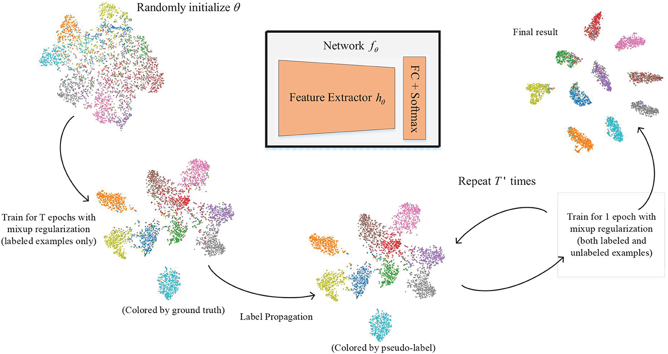
Figure 1. Overview of the proposed method. The colored points are the t-SNE visualization of the feature vectors extracted from Cifar10 train data by the same deep neural network in different training stages (we squeeze the 128-D feature vectors into 2-D plane coordinates using t-SNE). Starting from a randomly initialized network, we first train it with labeled data (l = 1,000) only and differential privacy to form a primitive network representation. Then, we perform label propagation and train the network on the entire dataset, with both handcraft labels and pseudo-labels. We repeat this process for T′ times until convergence.
3.3. Supervised mixup pre-training
In the early stage of the training process, the neural network f is composed of randomly initialized weight parameters. The output of the neural network is chaotic and has little semantic information about the input images. In previous studies, the network is pre-trained using the labeled samples by minimizing supervised cost only. Standard optimization techniques are employed in this procedure. The optimization target is the expectation of loss function ℓ over the labeled data distribution PD as follows:
where is a point distribution that is employed to estimate the true data distribution PD when labeled data set XL and correspondent label YL are given. With fewer labeled data in the SSL setting, the point distribution is hardly able to estimate the true data distribution PD, causing the model overfitting and degeneration. Previous studies take measures to mitigate this problem, using a larger learning rate and fewer pre-training epochs (Iscen et al., 2019). Other regularization techniques such as dropout and weight decay are adopted by Luo et al. (2018) and Miyato et al. (2019).
In this study, we introduce mixup (Zhang et al., 2018) in the pre-training procedure. Instead of simple point distribution, mixup proposes a vicinal distribution to estimate PD, whose generative process is summarized as follows:
where α is a hyperparameter α ∈ (0, ∞), which controls the strength of interpolation between data pairs. Notably, DM will degrade to DL as α → 0. We denote the mixup distribution as DM(DL, α). By replacing the DL with mixup distribution in Equation (3), we have as follows:
In a nutshell, we just randomly sample two data points each time and perform standard supervised training using the mixed data point. Notably, the interpolation between yi and yj is an interpolation between two one-hot encoded probability vectors. This modification does not influence the optimization process, which means any optimizer and network architecture can be applied with this regularization.
We summarize the benefits of introducing mixup mainly in two-folds as follows:
(1) Overfitting problem is greatly alleviated. While the output posterior probability of the classifier is forced to transit linearly from class to class, the decision boundaries between classes are pushed into the intermediate area, reducing the number of undesirable results when predicting outside the train examples. The experiments will demonstrate the test error of the pre-trained network is reduced by introducing mixup regularization.
(2) The internal representation of the classifier is encouraged to transit linearly as well as the output, leading to abstract representations in smooth and coherent feature space, and then more accurate label propagation is preformed based on sample distance in feature space.
3.4. Label propagation via nearest neighbor graph
Given a classification network f with pre-trained parameters θ, we clarify how to infer the possible label for unlabeled examples, which is employed to guide the SSL optimization process in the following subsection. First, we construct a graph based on network internal representations of all examples, and then, we apply label propagation on the graph to infer pseudo labels.
In most cases, the deep neural network can be seen as a sequence of non-linear layers or transformations, with each transformation giving an internal representation of the input. While the low-level representation captures more details of the input image, the high-level representation contains more semantic information about the input image, and the last layer maps the input feature into class probabilities. In a nutshell, network f can be decomposed as f = g ◦ h where is a feature extractor and g : ℝd ↦ ℝc is the output layer usually consisting of a fully-connected layer with softmax. We take h as a low-dimensional feature extractor and denote the feature vector for the i-th example as vi: = h(xi). We extract all features set of D as V = {v1, .., vl, vl+1, ..., vn} for similarity computation.
The next is to construct a graph on N data nodes. While computing the full N × N affinity matrix A may be intractable, we approximate it by constructing a nearest neighbor graph and only count the similarity between nodes and their k nearest neighbors. Thus, we create a graph with a sparse affinity matrix A ∈ ℝn × n and its elements as follows:
where NNk(vi) denotes the set of k nearest neighbors of vi in D, and s is the similarity function. The choice of s is quite flexible. Since we need to approximate the semantic similarity of two instances, we adopt the Gaussian similarity function with hyperparameter σ. Notably, approximate nearest neighbor (ANN) algorithms can be applied to accelerate the graph construction for large N.
Hereafter, let W : = A + AT be the symmetric affinity matrix and be its normalized counterpart, D is the diagonal degree matrix, in which the element is defined by . Further more, the volume of the graph is formulated as .
After defining those parameters, we are going to describe our LP algorithm by defining input and output as two n × c matrix Y, Z. Y is the matrix of the given label with rows {y1, ..., yl, yl+1, ...yn}, where the first l rows are corresponding one-hot encoded labels of each labeled example, and the rest are all zero vectors. Z is the desired class posterior probabilities which are solved by minimizing the following cost function:
Here, zi is the i-th row of matrix Z, is the normalized graph Laplacian and ∥·∥F is the Frobenius norm. The first term encourages smoothness where similar examples tend to induce the same predictions, and the last term attempts to maintain predictions for labeled examples (Zhou et al., 2003). In addition, the outlier which is indicated by a lower degree dii is forced to have a weak label in the second term. Thus, the degree of smoothness and weakness of outliers is controlled by weight parameters β and γ individually. To find the optimal solution of Z, we set the derivative of Equation (7) with respect to Z to 0 and obtain as follows:
Thus, the optimal Z is defined as follows:
Let and ignore the constant part in Equation (9). We have as follows:
Directly computing Z* by Equation (10) is often intractable for large n because the inverse matrix is not sparse, Instead, we use the conjugate gradient (CG) method to solve the linear system as follows:
This method is applicable because is a positive-definite matrix. The CG method has been adopted in many LP applications (Zhou et al., 2003; Gong et al., 2015; Tu et al., 2015; Iscen et al., 2019). Finally, the pseudo-label for an unlabeled example is given as follows:
Equation (11) is a hard assignment by evaluating the most confident class of each example; however, the contrast between classes can reflect the certainty of each example. Following Iscen et al. (2019), we associate a measure of confidence to each unlabeled example of calculating the entropy of Z:
where is the normalized counterpart of zi, in other words, , function H : ℝc ↦ ℝ is the entropy function.
3.5. Mixup regularization with differential privacy
Given the pseudo-label and confidence measure of all unlabeled data, we associate them with each example and denote the point distribution of unlabeled data as . To take the confidence coefficient into account, we propose the mixup distribution of unlabeled data as DMU whose generative process is summarized as follows:
In this generative process, the input data are interpolated randomly between two examples, while the pseudo-label and confidence score are interpolated with the same proportion as well.
The abundant unlabeled data are used in the training process by minimizing the following cost along with labeled data.
While the interpolation of labeled data can help form better network representation, in the unsupervised part, introducing interpolation of unlabeled data can lead to two benefits as follows: (1) The decision boundaries are pushed far away from unlabeled data, which are a desired property of low-density separation assumption. The model is forced to make neutral predictions in the middle zone of different samples or namely different clusters. (2) The clusters in hidden space are encouraged to have only one class of pseudo label, respectively. Considering the clusters in hidden space, if data points in one cluster are pseudo-labeled by two different classes, the mixup loss term will tear this cluster apart. The middle of this cluster is both encouraged to have neutral predictions as the interpolation of edge points or encouraged to have clear predictions as the middle points of the cluster.
Moreover, we employ differential privacy by directly adding noise to the latent representation of the deep neural network in the training progress:
where ϵ is randomly sampled from . This procedure is inspired by the Ladder network (Rasmus et al., 2015). By adding noise to its latent representation, the neural network will have more resistance to the dataset bias and form a more coherent latent space.
Finally, we finetune the network by minimizing the following objective function using both labeled and unlabeled data:
where λ is a coefficient that controls the effects of the unsupervised term.
3.6. Iterative training
We summarize our approach with the above definitions. Given a convolution neural network f with randomly initialized weights θ, we begin by training the network with mixup regularization for T epochs using the supervised loss term (Equation 5), and then, we start the following iterative process. First, we extract feature vector set V on the entire training set X and construct a nearest neighbor graph by computing the adjacency matrix via Equation (6). Second, we perform label propagation by solving the linear system (Equation 11) and assign pseudo-label and confidence score by Equations (12) and (13). Finally, we train the network for one epoch by minimizing the cost (Equation 17) on both labeled and unlabeled data set. This iterative process is repeated for T′ epochs.
The whole training process is summarized in Algorithm 1, where procedure Optimize() refers to the mini-batch optimization of the given loss term for one epoch. In our experiment, we randomly sample a mini-batch of data and perform mixup interpolation within this mini-batch, and this strategy is used to reduce I/O consumption and report no harm to the result in the study by Zhang et al. (2018). The procedure NearestNeighborGraph() refers to the nearest neighbor graph construction based on the feature vector set V and the computing of edge value in the graph.
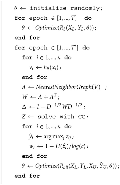
Algorithm 1. Mini-batch training with LP for SSL.
4. Experiments
In this section, we conduct our experiments with several standard image datasets commonly used in image classification. We first describe the datasets and our implementation details, and then, we compare the proposed method with the state-of-the-art methods. Finally, we conduct an ablation study to give a deep investigation into our method.
4.1. Datasets
We conduct experiments on three datasets, such as Cifar10, Cifar100, and Mini-imagenet. Cifar10 is widely used in related study, and Mini-imagenet is adopted by Iscen et al. (2019), to evaluate the proposed method on a large-scale dataset. Those datasets are commonly used in SSL setting by randomly taking a certain amount of labels and all image data to train the network and evaluate on the test set for fair a comparison with fully supervised methods, while the use of other labels in the training process is forbidden.
4.1.1. Cifar10, Cifar100
Cifar10 and Cifar100 datasets (Krizhevsky, 2009) are adopted in the evaluation process of previous SSL methods. The two datasets consist of small images of size 32 × 32. The training set of Cifar10 contains 50 k images, and its test set contains 10 k images, collected from 10 classes. Similar to Cifar10, Cifar100 has 50 and 10 k images for training and test, respectively, instead, Cifar100 collects images from 100 classes. For Cifar10, we randomly choose 50, 100, 200, and 400 images from each class, as the labeled images in our evaluation corresponding to 500, 1,000, 2,000, and 4,000 labels in total. For each class, we also choose 500 images as the validation images and employ the best model in validation to get the final performance on the test dataset. Following the common practice, we repeat the selection process 10 times, and for each time, we run the algorithm once on the dataset split and report mean error and standard deviation of test accuracy.
4.1.2. Mini-imagenet
Mini-imagenet was proposed by Gidaris and Komodakis (2018) for a few-shot learning evaluation, which is a simplified version of the Imagenet dataset. We adopt the same setting as the study by Iscen et al. (2019). Mini-imagenet consists of 100 classes with 600 images in each class, we randomly choose 500 images per class for the training set and use the remaining 100 images for testing.
4.2. Implementation details
4.2.1. Networks
We adopt a “13-layer” network for experiments on Cifar10 and Cifar100, which is a baseline used in all experiments in Table 1, and Resnet-18 is employed for experiments on Mini-imagenet. All of those networks consist of a feature extractor hθ, followed by a linear classification layer. The l2-normalization after the feature extractor in the study by Iscen et al. (2019) is canceled, which reported slightly harmful performance since we employ the Mahalanobis distance between features instead of the dot product as the similarity function.
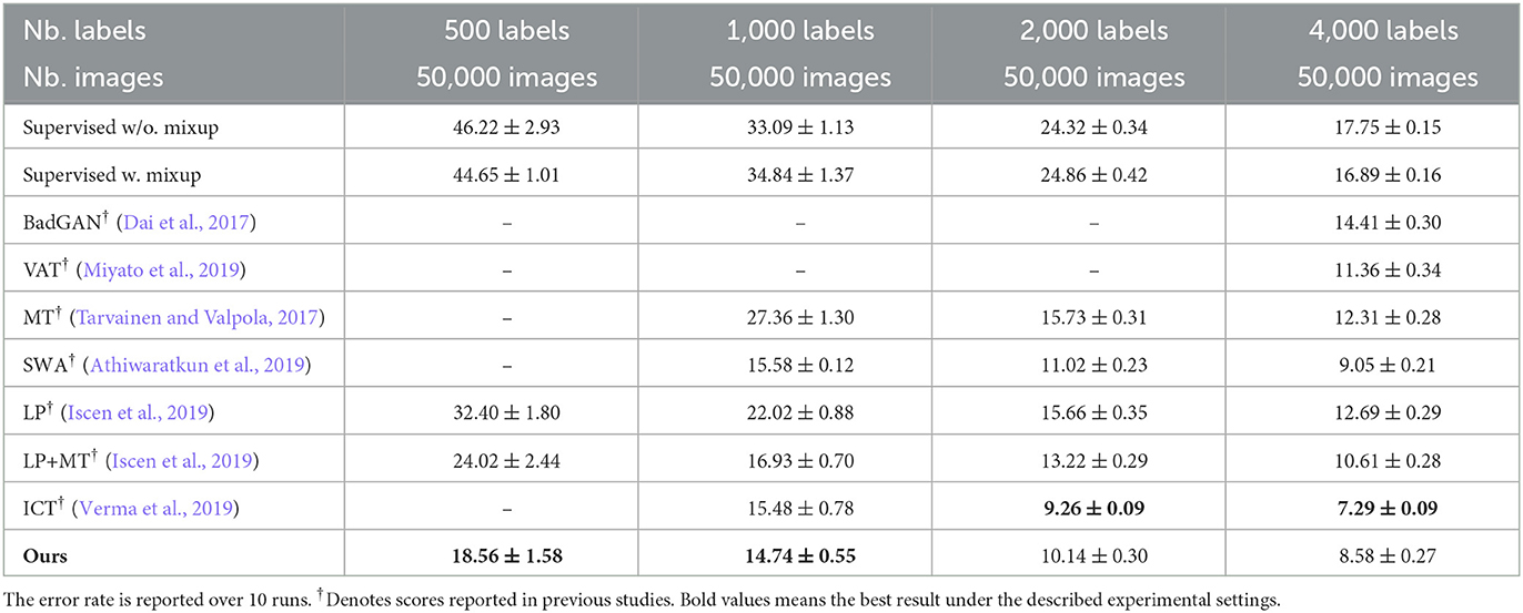
Table 1. Comparison with state-of-the-art methods on Cifar10 using 13-layer ConvNet network architecture.
4.2.2. Hyper-parameters
The following hyper-parameters are adopted in all experiments. First, we train the model with labeled data for 30 epochs, then we finetune the model with all data for 270 epochs for the experiments on Cifar10 and Cifar100 and 370 epochs for the experiments on Mini-imagenet. The training is performed using the SGD optimizer in all experiments. The learning rate is decayed from 0.1 to 0 with cosine annealing (Loshchilov and Hutter, 2016), and the momentum and weight decay parameters are set to 0.9 and 0.0001, respectively.
For the three hyperparameters, k, k1, k2 introduced in Section 3.5, and we set k = 10 in Equation (6) for fast graph construction and set k1 = 0.99, k2 = 0.0005 in Equation (11), where we implement the CG algorithm using the python sci-kit package. Other two hyperparameter mixup coefficients αsu and αunsu are set to 1.0 in all our experiments. We set the value of λ in Equation (17) to 10 for all experiments.
4.3. Comparison with state-of-the-art methods
In this section, we present a comparison with the state-of-the-art methods. We choose representative methods from three categories, such as generative SSL methods (BadGAN; Dai et al., 2017), consistency-based SSL methods [VAT; (Miyato et al., 2019), MT (Tarvainen and Valpola, 2017), and ICT (Verma et al., 2019)], and graph-based SSL methods (LP; Iscen et al., 2019). The performance of various methods on three datasets is represented in Tables 1–3, respectively.
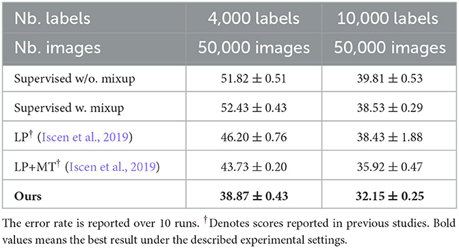
Table 2. Comparison with the state-of-the-art methods on Cifar100 using 13-layer ConvNet network architecture.
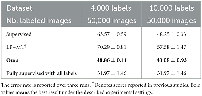
Table 3. Comparison with state-of-the-art methods on Mini-imagenet using the resnet-18 network.
The proposed method outperforms other methods with the same network architecture. On the Cifar10 dataset, our method achieves a significant error rate reduction (~20%) compared with our precedent method (Iscen et al., 2019), showing that our method exactly amends its weakness and successfully mitigates the performance gap between the graph-based SSL framework and other SSL methods. Compared with the best consistency-based method (Verma et al., 2019) to our knowledge, our method performs slightly weaker with 4,000 labels in total but outperforms it with fewer labeled images. This shows the advantage of traditional graph-based SSL learning that it can make more effective utilization of available labels, which are still applicable when it comes to modern deep learning architecture. We also try to use even fewer labels to evaluate the robustness of our method. Holding 500 labels (~1% of all), our method still achieves 18.56% error rate on the Cifar10 dataset.
4.4. Ablation studies
We conduct ablation studies to investigate the impact of mixup regularization on the pseudo-labels. To access the quality of pseudo-labels, accuracy is an important indicator. Despite this, we utilize the confidence score to calculate the weighted accuracy of pseudo-labels: . During the iterative optimization process, if the models are not capable of correcting wrong pseudo-labels, the confidence of those mistakes will increase and eventually get close to 1, leading to Accweighted ≈ Acc. The weighted accuracy indicator can reflect if the model really learns something useful from unlabeled images or if it just remembers the pseudo-labels. Figure 2 shows the progress of accuracy and the weighted accuracy of pseudo-labels throughout the training process. The experiments are conducted on Mini-imagenet with 100 labels per class. The results show that if no mixup regularization is applied or only applying mixup regularization on labeled data, the accuracy of pseudo-labels only increases in the beginning and tends to be stable in the following epochs, while the weighted accuracy curve keeps declining until getting close to the accuracy curve. These results imply that without regularization, the deep neural network just remembers the pseudo-labels due to its excessive representational ability. In contrast, our regularization method successfully alleviates such undesired phenomenon, and the accuracy of pseudo-labels is keep increasing during the training process.
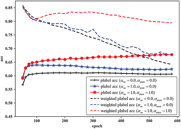
Figure 2. Pseudo-label accuracy and weighted pseudo-label accuracy with different mixup conditions on Mini-imagenet (10,000 labels are given in the training process, and accuracy is calculated according to ground truth). α = 0.0 means no mixup operation and α = 1.0 means mixup coefficient, λ is drawn from a uniform distribution. The results show that the applied regularization in both two losses greatly improves the pseudo-label accuracy during the iterative training process.
In Table 4, we compare the performance of Mini-imagenet. The results show that our method greatly reduces the error rate compared with the baseline method even on a high-resolution image dataset. To investigate the effectiveness of differential privacy in the proposed method, we vary the noise scale from 0 to 1.0 and report the performance on different datasets in Table 5. The results clearly show that the added noise reduces the error rate of the final model.
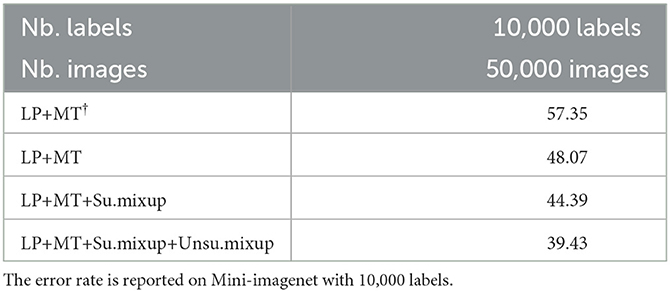
Table 4. Impact of mixup regularization on pair of labeled data points or unlabeled data points.
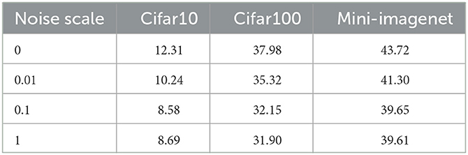
Table 5. Impact of varying the noise scale σ.
5. Conclusion and future work
In this study, we present a simple but effective regularization method in the graph-based SSL framework. Based on the previously proposed method that extends the traditional graph-based SSL framework for modern deep learning of image recognition, our study further strengthens this research line by introducing two critical measures as follows: imposing regularization on the latent space of the deep neural network and preventing the outlier data points from hurting the label propagation process. We show that our approach is effective and practical in utilizing unlabeled images via evaluation on both simple datasets of Cifar10 and Cifar100 and complex datasets with high resolution (Mini-imagenet). Furthermore, our method is computationally efficient and easy to implement the experiment on Mini-imagenet costs approximately 5h using a single NVIDIA 1080TI GPU. Our study also demonstrates differential privacy, which is an effective technique to constrain the excessive representation power of deep neural networks. Future study includes designing more delicate and effective regularization techniques in the SSL framework to further mitigate the performance gap between semi-supervised learning and supervised learning with all labels.
Data availability statement
The original contributions presented in the study are included in the article/supplementary material, further inquiries can be directed to the corresponding author.
Author contributions
All authors listed have made a substantial, direct, and intellectual contribution to the work and approved it for publication.
Funding
This research study was funded in part by the Defence Industrial Technology Development Program under grant No. JCKY2020604B004.
Conflict of interest
The authors declare that the research was conducted in the absence of any commercial or financial relationships that could be construed as a potential conflict of interest.
Publisher's note
All claims expressed in this article are solely those of the authors and do not necessarily represent those of their affiliated organizations, or those of the publisher, the editors and the reviewers. Any product that may be evaluated in this article, or claim that may be made by its manufacturer, is not guaranteed or endorsed by the publisher.
References
Athiwaratkun, B., Finzi, M., Izmailov, P., and Wilson, A. G. (2019). “There are many consistent explanations of unlabeled data: why you should average,” in Proceedings of the International Conference on Learning Representations (ICLR) (New Orleans, LA).
Belkin, M., Niyogi, P., and Sindhwani, V. (2006). Manifold regularization: a geometric framework for learning from labeled and unlabeled examples. J. Mach. Learn. Res. 7, 2399–2434.
Brock, A., Donahue, J., and Simonyan, K. (2018). “Large scale GAN training for high fidelity natural image synthesis,” in Proceedings of the International Conference on Learning Representations (ICLR) (Vancouver, BC).
Chapelle, O., Schölkopf, B., and Zien, A. (2006). Semi-Supervised Learning. The MIT Press. doi: 10.7551/mitpress/9780262033589.001.0001
Dai, Z., Yang, Z., Yang, F., Cohen, W. W., and Salakhutdinov, R. R. (2017). “Good semi-supervised learning that requires a bad GAN,” in Proceedings of the Advances in Neural Information Processing Systems (NIPS) (Long Beach, CA), Vol. 30.
Dwork, C., and Roth, A. (2014). The algorithmic foundations of differential privacy. Found. Trends Theor. Comput. Sci. 9, 211–407. doi: 10.1561/0400000042
Gidaris, S., and Komodakis, N. (2018). “Dynamic few-shot visual learning without forgetting,” in Proceedings of the IEEE Conference on Computer Vision and Pattern Recognition (Salt Lake City, UT), 4367–4375. doi: 10.1109/CVPR.2018.00459
Gong, C., Liu, T., Tao, D., Fu, K., Tu, E., and Yang, J. (2015). Deformed graph Laplacian for semisupervised learning. IEEE Trans. Neural Netw. Learn. Syst. 26, 2261–2274. doi: 10.1109/TNNLS.2014.2376936
Goodfellow, I., Pouget-Abadie, J., Mirza, M., Xu, B., Warde-Farley, D., Ozair, S., et al. (2014). “Generative adversarial nets,” in Proceedings of the Advances in Neural Information Processing Systems (NIPS) (Montreal, QC).
Gulrajani, I., Ahmed, F., Arjovsky, M., Dumoulin, V., and Courville, A. C. (2017). “Improved training of wasserstein GANs,” in Proceedings of the Advances in Neural Information Processing Systems (NIPS) (Long Beach, CA), Vol. 30.
Iscen, A., Tolias, G., Avrithis, Y., and Chum, O. (2019). “Label propagation for deep semi-supervised learning,” in Proceedings of the IEEE/CVF Conference on Computer Vision and Pattern Recognition (CVPR). (Long Beach, CA). doi: 10.1109/CVPR.2019.00521
Jebara, T., Wang, J., and Chang, S.-F. (2009). “Graph construction and b-matching for semi-supervised learning,” in Proceedings of the International Conference on Machine Learning (ICML) (Montreal, QC), 441–448. doi: 10.1145/1553374.1553432
Kamnitsas, K., Castro, D., Le Folgoc, L., Walker, I., Tanno, R., Rueckert, D., et al. (2018). “Semi-supervised learning via compact latent space clustering,” in International Conference on Machine Learning (Stockholm), 2459–2468.
Kingma, D. P., Mohamed, S., Jimenez Rezende, D., and Welling, M. (2014). “Semi-supervised learning with deep generative models,” in Proceedings of the Advances in Neural Information Processing Systems (NIPS) (Montreal, QC), Vol. 27.
Kingma, D. P., and Welling, M. (2013). Auto-encoding variational bayes. arXiv preprint arXiv:1312.6114.
Kobyzev, I., Prince, S. J., and Brubaker, M. A. (2020). Normalizing flows: an introduction and review of current methods. IEEE Trans. Pattern Anal. Mach. Intell. 43, 3964–3979. doi: 10.1109/TPAMI.2020.2992934
Krizhevsky, A. (2009). Learning multiple layers of features from tiny images (Master's thesis). University of Toronto, Toronto, ON, Canada.
Li, G., Ota, K., Dong, M., Wu, J., and Li, J. (2020). Desvig: decentralized swift vigilance against adversarial attacks in industrial artificial intelligence systems. IEEE TII 16, 3267–3277. doi: 10.1109/TII.2019.2951766
Li, G., Wu, J., Li, S., Yang, W., and Li, C. (2022). Multi-tentacle federated learning over software-defined industrial internet of things against adaptive poisoning attacks. IEEE Trans. Indus. Inform. 19, 1260–1269. doi: 10.1109/TII.2022.3173996
Loshchilov, I., and Hutter, F. (2016). SGDR: Stochastic gradient descent with warm restarts. arXiv preprint arXiv:1608.03983.
Luo, Y., Zhu, J., Li, M., Ren, Y., and Zhang, B. (2018). “Smooth neighbors on teacher graphs for semi-supervised learning,” in Proceedings of the IEEE/CVF Conference on Computer Vision and Pattern Recognition (CVPR) Salt Lake City, UT. doi: 10.1109/CVPR.2018.00927
Maaløe, L., Sønderby, C. K., Sønderby, S. K., and Winther, O. (2016). “Auxiliary deep generative models,” in Proceedings of the International Conference on Machine Learning (ICML) (New York, NY), Vol. 48, 1445–1453.
Makhzani, A., Shlens, J., Jaitly, N., Goodfellow, I., and Frey, B. (2015). Adversarial autoencoders. arXiv preprint arXiv:1511.05644.
Miyato, T., Maeda, S.-I., Koyama, M., and Ishii, S. (2019). Virtual adversarial training: a regularization method for supervised and semi-supervised learning. IEEE Trans. Pattern Anal. Mach. Intell. 41, 1979–1993. doi: 10.1109/TPAMI.2018.2858821
Radford, A., Metz, L., and Chintala, S. (2015). Unsupervised representation learning with deep convolutional generative adversarial networks. arXiv preprint arXiv:1511.06434.
Rasmus, A., Berglund, M., Honkala, M., Valpola, H., and Raiko, T. (2015). “Semi-supervised learning with ladder networks,” in Proceedings of the Advances in Neural Information Processing Systems (NIPS) (Montreal, QC), Vol. 28.
Ren, G., Wu, J., Li, G., Li, S., and Guizani, M. (2022). Protecting intellectual property with reliable availability of learning models in ai-based cybersecurity services. IEEE TDSC 1–18. doi: 10.1109/TDSC.2022.3222972
Sajjadi, M., Javanmardi, M., and Tasdizen, T. (2016). “Regularization with stochastic transformations and perturbations for deep semi-supervised learning,” in Proceedings of the Advances in Neural Information Processing Systems (NIPS) (Barcelona), 1163–1171.
Salimans, T., Goodfellow, I., Zaremba, W., Cheung, V., Radford, A., and Chen, X. (2016). “Improved techniques for training GANs,” in Proceedings of the Advances in Neural Information Processing Systems (NIPS) (Barcelona), Vol. 29.
Tarvainen, A., and Valpola, H. (2017). “Mean teachers are better role models: weight-averaged consistency targets improve semi-supervised deep learning results,” in Proceedings of the Advances in Neural Information Processing Systems (NIPS) (Long Beach, CA), 1195–1204.
Tu, E., Yang, J., Kasabov, N., and Zhang, Y. (2015). Posterior distribution learning (PDL): a novel supervised learning framework using unlabeled samples to improve classification performance. Neurocomputing 157, 173–186. doi: 10.1016/j.neucom.2015.01.020
Verma, V., Lamb, A., Kannala, J., Bengio, Y., and Lopez-Paz, D. (2019). “Interpolation consistency training for semi-supervised learning,” in Proceedings of the International Joint Conference on Artificial Intelligence (IJCAI) (Macao), 3635–3641. doi: 10.24963/ijcai.2019/504
Yu, B., Wu, J., Ma, J., and Zhu, Z. (2019). “Tangent-normal adversarial regularization for semi-supervised learning,” in Proceedings of the IEEE/CVF Conference on Computer Vision and Pattern Recognition (CVPR) (Long Beach, CA), 10676–10684. doi: 10.1109/CVPR.2019.01093
Zhang, H., Cisse, M., Dauphin, Y. N., and Lopez-Paz, D. (2018). “Mixup: beyond empirical risk minimization,” in Proceedings of the International Conference on Learning Representations (ICLR) (Vancouver, BC).
Keywords: deep semi-supervised learning, label propagation, differential privacy, robust learning, mixup data augmentation
Citation: Yan Z, Li S, Duan Z and Zhao Y (2023) Robust deep semi-supervised learning with label propagation and differential privacy. Front. Comput. Sci. 5:1114186. doi: 10.3389/fcomp.2023.1114186
Received: 02 December 2022; Accepted: 20 April 2023;
Published: 24 May 2023.
Edited by:
Chaofeng Zhang, Advanced Institute of Industrial Technology, JapanReviewed by:
Chong Di, Qilu University of Technology, ChinaJianwen Xu, Muroran Institute of Technology, Japan
Copyright © 2023 Yan, Li, Duan and Zhao. This is an open-access article distributed under the terms of the Creative Commons Attribution License (CC BY). The use, distribution or reproduction in other forums is permitted, provided the original author(s) and the copyright owner(s) are credited and that the original publication in this journal is cited, in accordance with accepted academic practice. No use, distribution or reproduction is permitted which does not comply with these terms.
*Correspondence: Shenghong Li, c2hsaUBzanR1LmVkdS5jbg==