Real-Time Music Following in Score Sheet Images via Multi-Resolution Prediction

The task of real-time alignment between a music performance and the corresponding score (sheet music), also known as score following, poses a challenging multi-modal machine learning problem. Training a system that can solve this task robustly with live audio and real sheet music (i.e., scans or score images) requires precise ground truth alignments between audio and note-coordinate positions in the score sheet images. However, these kinds of annotations are difficult and costly to obtain, which is why research in this area mainly utilizes synthetic audio and sheet images to train and evaluate score following systems. In this work, we propose a method that does not solely rely on note alignments but is additionally capable of leveraging data with annotations of lower granularity, such as bar or score system alignments. This allows us to use a large collection of real-world piano performance recordings coarsely aligned to scanned score sheet images and, as a consequence, improve over current state-of-the-art approaches.

1 Introduction

Score following or real-time audio-to-score alignment aims at synchronizing musical performances (audio) to the corresponding scores (the printed sheet music from which the musicians are presumably playing) in an on-line fashion. In other words, the task is for a machine to listen to a musical recording or performance and be able to follow along in the sheet music of the respective piece, with a certain robustness to peculiarities of the particular live performance ‐ such as unpredictable tempo and tempo changes, mistakes by the performing musicians, etc. Score following systems can be used for a variety of applications including automatic page turning for musicians (Arzt et al., 2008), displaying synchronized information in concert halls (Arzt et al., 2015), and automatic accompaniment for solo musicians (Cont, 2010; Raphael, 2010; Cancino-Chacón et al., 2017a). Existing approaches usually rely on symbolic computer-readable score representations such as MIDI or MusicXML (Orio et al., 2003; Dixon, 2005; Cont, 2006; Nakamura et al., 2015; Arzt, 2016). However, these kinds of representations are often not readily available and have to be either created by hand or automatically extracted from the printed scores using optical music recognition (OMR) (Calvo-Zaragoza et al., 2019). While the former is time-consuming and tedious (think of typesetting an entire Beethoven sonata or Mahler symphony), automatic extraction via OMR may require substantial manual corrections as well, depending on the complexity and quality of the score.

Recent advances in deep learning promise to overcome this problem by permitting us to perform score following directly on score sheet images (printouts, scans), which does not require any pre-processing or manually created score representations. More specifically, in previous work we have shown how neural networks can be trained to simultaneously listen to an incoming musical performance (audio) and read along in the score (image) (Henkel et al., 2019, Henkel et al., 2020; Henkel and Widmer, 2021), thus opening up a challenging multi-modal machine learning problem.

In this article we build upon, and extend, our current state-of-the-art approach that frames sheet-image-based score following as a multi-modal conditional bounding box regression task (Henkel and Widmer, 2021). The task here is for a neural network to predict, at any time, the most likely position in the sheet image, in the form of a bounding box around the notes that match the incoming audio signal. In addition to the intrinsic difficulty of this task, with different ways in which the same musical passage can be typeset and played, we also face a severe data problem: training such a network requires large amounts of fine-grained annotations between note positions on the sheet image and in the audio. Obtaining such information at this level of precision via manual annotation is factually impossible, at least in the acoustic domain. That is why current research uses synthetic data for this purpose, where score and audio are automatically rendered, in the visual and in the audio domain, from an underlying machine-readable version of the score (e.g., in the form of MusicXML files), so that the precise positions and time points of notes on the sheet and in the audio, respectively, are precisely known. As there is only a limited supply of data with such precise annotations, we propose a new model that learns to make predictions at several levels of granularity simultaneously, jointly predicting note-, bar- and system-level alignments in the sheet image. That makes it possible to leverage additional data with less fine-grained annotations (i.e., only marked at the level of bars or staff systems), which are easier to come by. This formulation allows us to use real-world data: a collection of scanned sheet images and real piano music recordings that were annotated in a semi-automated way, with relatively little effort. Using this data, we conduct large-scale experiments to investigate the generalization capabilities of our proposed system in the audio as well as in the sheet-image domain.

2 Related Work

Approaches to score following are mainly categorized into methods that require symbolic computer-readable score representations (e. g., Dynamic Time Warping (DTW) or Hidden Markov Models) and those that directly work with images of scores by applying deep learning techniques. In this article, we specifically target sheet-image-based approaches; in other words, input to the system will be the score of a piece, in the form of printed or scanned pages, i.e., images; and a live audio stream representing the music currently being played. In the following, we focus on this latter, harder problem, and give a brief overview of current approaches and their drawbacks.

The first method in this area was presented by Dorfer et al. (2016), who proposed to treat the task as a one-dimensional localization problem. The authors train a multi-modal convolutional neural network (CNN) to match short audio and sheet image excerpts. To that end, the sheet image excerpt is discretised into k bins and the most likely bin that matches the audio excerpt has to be predicted. In follow-up work, score following is formulated as a reinforcement learning (RL) problem (Dorfer et al., 2018b; Henkel et al., 2019), reaching high performance on synthetic polyphonic piano music. Here, RL agents are trained to follow along live performances by adapting their reading speed, i. e., how fast they want to move forward or backward in an unrolled representation of the sheet image. The authors further conduct first experiments using real-world piano recordings, showing that RL agents are able to generalize to some extent to different recording conditions.

Both approaches rely on a cumbersome preprocessing step in the form of score unrolling. During that process, one has to first detect all systems on a sheet image (see Figure 1 for an explanation of the basic musical score concepts), cut them out from the full page and stitch them together into a long sequence. This sequence is then fed to the score following system step by step, i. e., as short audio and sheet image excerpts (see Figure 2). However, unrolling the score and working with audio/image excerpts poses two problems. First, it again introduces a dependency on an external system to detect staves on the page, e. g., an OMR system, which we initially wanted to get rid of. Second, and even more severe, the currently selected sheet image excerpt has to (at least partially) correspond to the incoming audio excerpt. If this is not the case anymore, e. g., due to tracking errors, the system is not able to produce proper predictions and gets lost.

FIGURE 1

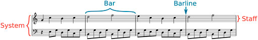
FIGURE 1. Example of a single system with two staves and 4 bars (or measures). Note that this is also an illustration of ambiguities in sheet images. Bars 2 and 4 share the same musical content and without a large enough temporal context, a score follower will not be able to distinguish between them. However, if it is able to remember that it has already encountered the first sequence of notes in bar 2 then it can correctly predict the current position to be in the last bar.

FIGURE 2

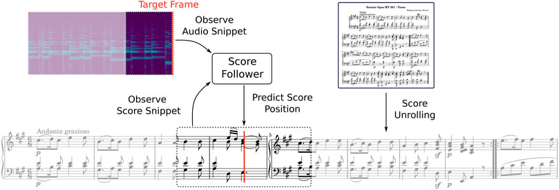
FIGURE 2. Sheet-image based score following using unrolled score representations. First, the systems on a sheet image page must be detected, cut out and stitched together to a long (unrolled) sequence. The score following system then observes a small excerpt of the full score sequence as well as the audio (usually the last 2 seconds). Based on this input, the score follower has to predict the most likely position in the sheet excerpt matching the target audio frame.

To overcome the need for unrolled score representations, Henkel et al. (2020) treat score following as a referring image segmentation task. In computer vision, the goal of referring image segmentation is to segment an object in a given image based on some language expression (Hu et al., 2016). For example, consider an image with two persons, where one wears a red shirt and the other wears a blue one. Given the referring expression “the person with the red shirt”, the system has to identify, i. e., segment, the person with the red shirt in the image. For music score following in this setup the referring expression would be the audio signal heard so far, up until the current point in time, and the task is then to mark the region around the note location in the complete score sheet image that corresponds to the just heard sounds. This segmentation is performed using a conditional U-Net architecture that applies Feature-wise Linear Modulation (FiLM) (Perez et al., 2018) layers to combine the audio and sheet image.

While the former approaches directly process the raw input using neural networks, another line of research makes use of intermediate representations. Shan and Tsai. (2020) propose to first transcribe the audio signal into discrete note events, represented in MIDI format or so-called “piano roll” format. Subsequently, the piano roll and the score sheet image are transformed to a common representation called bootleg score (Tanprasert et al., 2019). Given this common space, the authors then apply a variant of Dynamic Time Warping specifically designed to handle jumps and repeats in the music. Since this approach requires the full audio to be available up front (off-line alignment), it is not directly applicable to our on-line setup; however, using a potentially more robust intermediate representation such as a bootleg score might be beneficial for generalization.

3 Multi-Modal Bounding Box Prediction for Score Following

In (Henkel and Widmer, 2021), we present a new approach, framing score following as a multi-modal bounding box regression task and proposing a conditional neural network architecture based on the family of YOLO object detectors (Redmon et al., 2016; Redmon and Farhadi, 2017). This is inspired by object detection, where the goal is to predict bounding boxes around all known objects in an image. However, we need to consider a conditional setup: the task is not to predict all bounding boxes for all objects, but only a particular one that matches an input query. In our case, this query is an audio signal and the target to predict is a bounding box around the notes or chords in the sheet image that correspond to the notes that have just started in the audio (cf. Figure 3). This is implemented as a bounding box regression task, where the system has to predict x, y center coordinates as well as the width and height of the bounding box.

FIGURE 3

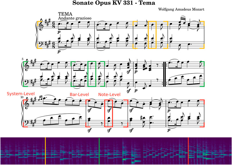
FIGURE 3. Data Annotation with three different granularities: system-, bar-, and note-level. For each frame in the audio, the model has to predict the most likely system, bar and note position in the sheet image matching the audio up until the current point in time. The colored bars in the spectrogram mark the onset times in the audio corresponding to the (note-level) ground truth bounding boxes in the sheet image.

In the following, we describe the Conditional YOLO network architecture that we designed for this purpose, and that will also be the basis for the new, multi-granularity (or joint alignment) prediction model that we will describe in Section 4. In the subsequent Section 5, a series of systematic experiments will then be presented that demonstrate both how this Conditional YOLO approach improved over the previous state of the art described above, and how extending it to a multi-granularity prediction model can lead to substantial additional improvement.

3.1 Conditional YOLO

Table 1 and Figure 4 depict our Conditional YOLO network architecture and its building blocks. The architecture consists of several downscaling and upscaling blocks in combination with Feature-wise linear modulation (FiLM) layers (Perez et al., 2018). As input the network is presented with a 1 × 416 × 416 sheet image, which is first processed by a so-called Focus or SpaceToDepth (Ridnik et al., 2020) layer. This layer splits the input from 1 × 416 × 416 to 4 × 208 × 208 and subsequently applies a 16 × 3 × 3 convolution, layer normalization (Ba et al., 2016) and ELU activation (Clevert et al., 2016), with the purpose of reducing the input size and improving the overall computation speed.

TABLE 1

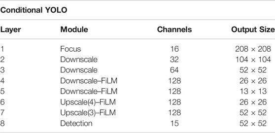
TABLE 1. The conditional YOLO architecture consists of four Downscale and two Upscale blocks as depicted in Figure 4. Upscale blocks concatenate the input from a previous layer given in parentheses, e. g., layer 6 takes the output of layer 4 as additional input. FiLM indicates that the conditional layer is active within a block. The Detection layer has 15 outputs for each spatial position in the 52 × 52 output grid (5 values for each of the three anchors which are used to compute the final bounding boxes (see Eq. 2).

FIGURE 4

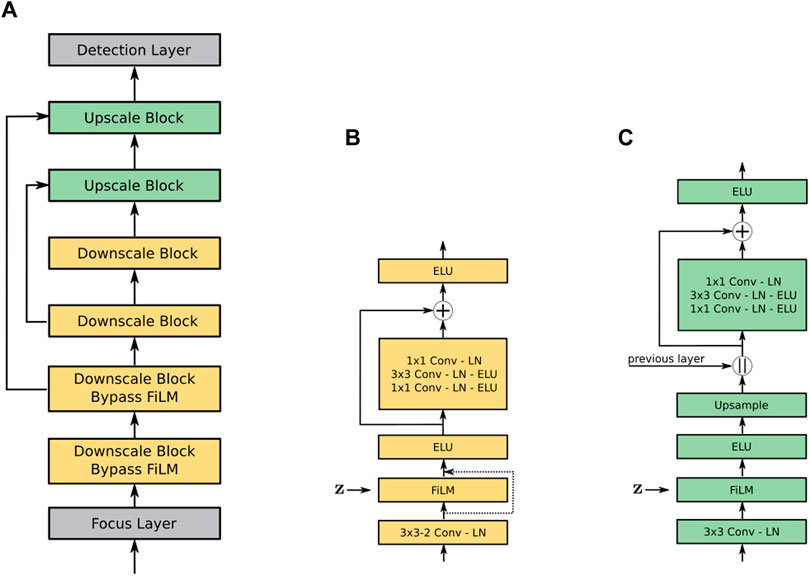
FIGURE 4. Conditional YOLO architecture (A) and its building blocks (B, C). The Downscale block (B) applies a 3 × 3 convolution with a stride of 2, halving the spatial dimension of the input feature maps. The FiLM layer is optional and bypassed in the first two Downscale blocks, i. e., the output of the convolutional layer after normalization is directly fed to the subsequent activation function. In the Upscale block, nearest neighbour up-sampling is applied by a factor of 2 and the feature maps from a given previous layer are concatenated channel-wise. The residual connection in both blocks serves as a bottleneck, reducing the number of parameters as the 3 × 3 convolution is performed with only half the number of output channels, e. g., 64 × 1 × 1, 64 × 3 × 3 and 128 × 1 × 1.

The following Downscale blocks reduce the input size by two at each layer, which results in feature maps of different resolutions (104 × 104, 52 × 52, 26 × 26, 13 × 13; see Table 1). Each block has an optional FiLM layer, which combines the visual features from the sheet image and the external query in the form of the encoded audio signal. The FiLM layer is defined as

$f_{\text{FiLM}}\left(\mathbf{x}\right)=\mathbf{s}\left(\mathbf{z}\right)\cdot \mathbf{x}+\mathbf{t}\left(\mathbf{z}\right),(1)$

where x are the input feature maps from a previous convolutional layer, z is a conditioning vector representing the query, and s(⋅) and t(⋅) are learned linear functions to scale and translate x. As depicted in Figure 4B, the FiLM layer can be bypassed, which we do for the first two blocks. The idea behind this is to learn a more general representation in the lower layers of the network, while specializing in later ones.

In the Upscale blocks, the lower resolution feature map of a previous layer is up-sampled by a factor of two, concatenated to a feature map of the same size from an earlier layer and eventually passed to the Detection layer after the last block. The resolution after the last up-sampling operation is 52 × 52, which will form the final output grid.

For each spatial position in this grid, the Detection layer predicts 15 output values, 5 for each of three “anchor boxes”. These anchor boxes are alternative pre-defined box templates that reflect our prior assumptions about reasonable bounding box widths and heights, to be customized by the specific parameters predicted by the network (see next paragraph and Figure 5). Remember that in our case a bounding box encloses notes or chords in the sheet image, where the height corresponds to the height of the system the notes are in and the width is arbitrarily chosen to be 30 pixels. The three anchor boxes we are using are (11, 26), (11, 34), (11, 45), with the two values denoting the anchor width and height, respectively. The width of 11 is defined for the down-scaled image (adapted from 30 pixels in full resolution) and the height values are determined using k-means clustering on the training set bounding boxes as explained in (Redmon and Farhadi, 2017). (The above applies to note-level bounding boxes as used in our previous work. The extension of the method to bar- and measure-level predictions will be described in Section 4 below.)

FIGURE 5

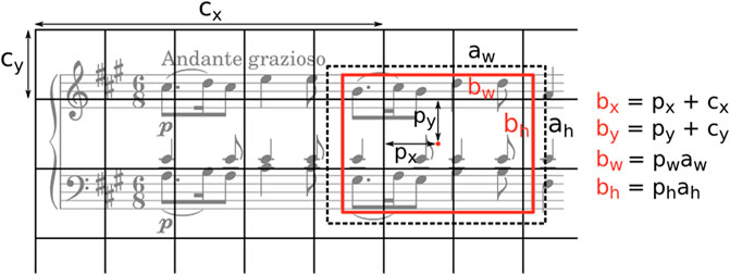
FIGURE 5. Anchor-based bounding box prediction. The network predicts relative box coordinates (p_x, p_y) for each grid cell (offset from the top left corner by c_x, c_y) as well as width and height values (p_w, p_h) to scale the anchor (a_w, a_h) (visualized as a dashed rectangle). The resulting bounding box is depicted in red. For the computation of p_x, p_y, p_w, p_h see Eq. 2. Figure inspired by (Redmon and Farhadi, 2017).

The 5 ouputs for each anchor are define as follows. The first two correspond to the offsets p_x, p_y for the center coordinates of the bounding boxes. Together with the spatial grid position, these will be used to compute the final coordinates in the original image (cf. Figure 5). The next two outputs are width and height values p_w, p_h to scale the anchor a_w, a_h and the last output is an “objectness” or confidence score p_o predicting the Intersection over Union (IoU) between the predicted and ground truth bounding box. The idea behind this score is that it should reflect how well the predicted box fits the ground truth, and during inference this allows us to filter the most likely positions in the sheet image matching the given query.

For the computation of p_x, p_y, p_w, p_h we deviate from (Redmon and Farhadi, 2017), and calculate them as

$\begin{array}{c}\hfill p_x=2\sigma \left(t_x\right)-0.5\\ \hfill p_y=2\sigma \left(t_y\right)-0.5\\ \hfill p_w={\left(2\sigma \left(t_w\right)\right)}^2\\ \hfill p_h={\left(2\sigma \left(t_h\right)\right)}^2\\ \hfill p_o=\sigma \left(t_o\right),\end{array}(2)$

where t_x, t_y, t_w, t_h, t_o are the raw network output values, and σ is the sigmoid function. Scaling the sigmoid output for the computation of p_x, p_y eliminates grid sensitivity (Bochkovskiy et al., 2020), otherwise t_x and t_y would need to take on extremely high or low values for the final bounding box coordinates to fall on the grid cell borders. In contrast to the unrestricted anchor scalers in (Redmon and Farhadi, 2017) we use a bounded formulation, which showed to improve training stability in practice.¹

3.2 Query Encoding

The initial query to our system is a raw audio signal, with a sample rate of 22.05 kHz. This signal is then processed using a Short-time Fourier-transform (STFT) with a Hann window of size 2048 and a hop size of 1102, resulting in approximately 20 frames per second. We further transform each frame with a logarithmic filterbank processing frequencies between 60 Hz and 6 kHz, which results in as spectrogram output with 78 log-frequency bins.

To encode the spectrogram, we use the CNN encoder depicted in Table 2, which takes the 40 latest audio frames and projects them to a 32 dimensional vector x. As shown in (Henkel et al., 2020), only encoding 40 frames of audio (roughly 2 s) is not enough to form reliable predictions. The main reason for this are the ambiguities within the sheet image when an audio excerpt could correspond to multiple positions in the sheet image (cf. Figure 1). To incorporate a longer temporal audio context, we use an LSTM layer (Hochreiter and Schmidhuber, 1997) with 64 hidden units on top of the encoded audio vector. The hidden state of the LSTM is updated every 40 frames, and the final conditioning vector z used in the FiLM layer is defined as

$\mathbf{z}=f\left(\left[\mathbf{h};\mathbf{x}\right]\right),(3)$

where f is a fully connected layer of size 128 with layer normalization and ELU activation, h refers to the hidden state vector of the LSTM, and [h; x] indicates a vector concatenation between the hidden state h and the latest 40 audio frames encoded into x.

TABLE 2

TABLE 2. CNN spectrogram encoder. Conv(f, p, s)-k denotes a convolutional layer with k f × f kernels, padding of p and stride s. We use layer normalization (LN) (Ba et al., 2016), the ELU activation function (Clevert et al., 2016) and max pooling (MP) with a pool size of 2 × 2. For input normalization we use a batch normalization (Ioffe and Szegedy, 2015) layer, to learn mean and standard deviation parameters for each frequency band similar to (Grill and Schlüter, 2017). Note that there are no affine transformation parameters γ and β in this normalization layer.

4 A New Approach: Joint Alignment Prediction at Several Granularity Levels

As already discussed in the introduction, one issue with our Conditional YOLO model described above ‐ and indeed with any approach to multi-modal score following that aims at aligning audio to sheet images ‐ is the dependency on precise note-level alignments, i. e., for each timestep in the audio we need to know the exact note position in the image. Since this is very time consuming to annotate, only a limited amount of such training data is available (which we will explain in more detail in Section 5.2). To overcome this problem, we propose a model that does not rely on note-level alignments only, but further leverages data with system and bar annotations which are easier and less time consuming to obtain. As shown in Figure 3, the goal of our proposed model is now to jointly predict bounding boxes for the specific note(s), bar and system corresponding to the current timestep. During training we assume bar- and system-level alignments to be always available, whereas the note-level alignments are optional.

We implement the joint alignment prediction by using three of the aforementioned Detection layers, each of which is responsible for outputting the prediction at a specific alignment level (see Figure 6). Each detection layer requires a pre-defined set of anchors. While we keep the same anchors as before for the first layer to predict note position bounding boxes, we use (61, 32), (77, 40), (148, 34) for bar and (249, 33), (267, 33), (267, 40) for system bounding boxes. These are again determined using k-means clustering on the training set bounding boxes, reflecting our prior assumption regarding bounding box sizes.

FIGURE 6

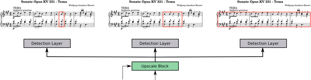
FIGURE 6. Joint alignment prediction at several granularity levels. Each Detection layer is responsible for a specific alignment type ‐ either notes, bars or systems, and takes the same input from the last Upscale block as shown in Figure 4. Note that while we only visualize the prediction for an excerpt of a score, the actual prediction is based on a full page.

The training objective for the conditional YOLO models consists of two parts, a mean-squared-error loss to learn the bounding box predictions and a logistic regression loss to predict the “objectness” score of the boxes. Remember that this score reflects the intersection over union (IoU) between a predicted bounding box and the ground truth, i. e., a prediction that has a perfect overlap with the ground truth should yield a score of 1.0 (Redmon and Farhadi, 2017).

The loss for the bounding boxes of a specific Detection layer l is defined as

${\text{loss}}_{\text{box}}^{\left(l\right)}={\mathrm{\lambda }}_{\text{box}}^{\left(l\right)}\frac{1}{|BC|}\sum _{i\in BC}\left[{\left(p_{x_i}-{\widehat{p}}_{x_i}\right)}^2+{\left(p_{y_i}-{\widehat{p}}_{y_i}\right)}^2+{\left(p_{w_i}-{\widehat{p}}_{w_i}\right)}^2+{\left(p_{h_i}-{\widehat{p}}_{h_i}\right)}^2\right],(4)$

where ${\lambda }_{\text{box}}^{(l)}$ is a scalar to weight the loss, p_* and ${\widehat{p}}_{*}$ are ground truth and predictions for bounding box parameters (see Eq. 2) and BC is the set of all possible bounding box candidates for grid cells where an object is present. This means that grid cells without a note, bar or system are not considered by the loss function.

Similarly, the loss for the objectness score is given as

${\text{loss}}_{\text{obj}}^{\left(l\right)}=-{\lambda }_{\text{obj}}^{\left(l\right)}\frac{1}{|C|}\sum _{c\in C}\left({\text{IoU}}_c\log p_{o_c}+\left(1-{\text{IoU}}_c\right)\log \left(1-p_{o_c}\right)\right),(5)$

with ${\lambda }_{\text{obj}}^{(l)}$ being a scalar to weight the loss term, p_o the predicted objectness score, C the set of all possible bounding boxes for all grid cells, and IoU the intersection over union between predicted and ground truth box in a given cell. In case there is no object present in a cell (and thus no ground truth box available), the IoU is assumed to be 0.

The final loss term is then computed by summing over all detection layers l ∈ L

$\text{loss}=\sum _{l\in L}\left({\text{loss}}_{\text{box}}^{\left(l\right)}+{\text{loss}}_{\text{obj}}^{\left(l\right)}\right).(6)$

In our experiments, we have a either a single detection layer to only predict note-level alignments, or three when note-, bar-, and system-level alignments are predicted. To balance the loss terms, ${\lambda }_{\text{box}}^{(l)}$ is set to 0.1 for all layers, and ${\lambda }_{\text{obj}}^{(l)}$ is set to 10 for the first layer, and 1 for the remaining ones. This should encourage the network to focus more on correctly predicting the note positions in the sheet image.²

5 Experiment Setup

In the following section, we introduce our experimental setup as well as the data used to explore the generalization capabilities of several sheet-image-based score following approaches. In particular, we consider three methods from the literature as explained in Section 2 as well as our approaches introduced in Sections 3 and 4.

5.1 Models

The first baseline is the aforementioned one-dimensional localization model as introduced in (Dorfer et al., 2016), which is referred to as MM-Loc. In contrast to the other approaches, this method is not completely on-line capable, but looks ahead roughly 0.7 s into the future. Our second baseline is the best reinforcement learning agent from (Henkel et al., 2019), which we refer to as RL. Both of these methods rely on unrolled score representations. We prepare those upfront using ground truth annotations from the scores, to evaluate the baselines under optimal conditions. As a further baseline we use the Conditional UNet for full page tracking that was introduced in (Henkel et al., 2020). We refer to this approach as CUNet.

Next, we use a plain Conditional YOLO that only predicts note-level alignments and one that additionally predicts system- and bar-level alignments as described in Sections 3 and 4. We call these CYOLO and CYOLO-SB, respectively. Given that CYOLO-SB is able to also handle data without note-level alignments, we further investigate whether additional training data with only system and bar alignments can be used to improve the generalization performance of such a model. In the following, we refer to this as CYOLO-SB + A.³

5.2 Dedicated Datasets

In the experiments, we are interested in two specific questions: how effective are current score following methods for sheet images in generalizing to real-world audio conditions, and how well do they handle scanned real sheet images? To answer these questions, we consider different types of datasets that allow us to treat them separately as well as in combination.

The main data source for sheet-image based score following research is the Multi-modal Sheet Music Dataset (MSMD) (Dorfer et al., 2018a). This polyphonic piano music dataset offers alignments between note head coordinate positions in the score sheet image and a MIDI score representation. The scores are typeset with Lilypond⁴ and for training purposes the MIDI representation is rendered to audio using Fluidsynth.⁵ Since the dataset is inherently synthetic with homogeneous and clean score images and without any performance variations in the audio, it does not allow one to precisely assess generalization to real-world conditions (i. e., audio recordings and scanned or photographed score pages) and is mainly used for training the score following systems. Additionally, the test split of this dataset will serve as a baseline to test the score following systems under optimal conditions.

To address our first question ‐ generalization to real audio recordings of (potentially expressive) performances –, we use a collection of actual piano recordings aligned to a subset of the MSMD test split (Henkel et al., 2019). Since this dataset still consists of clean typeset score images it allows us to investigate generalization in the audio domain without the influence of different sheet image variations. The dataset will be called MSMD–Rec hereafter.

For the second question – generalization to real sheet images –, we gather a collection of scanned scores aligned to musical performances from two major data sources, the Magaloff Corpus (Flossmann et al., 2010) and the Zeilinger Dataset (Cancino-Chacón et al., 2017). The Magaloff Corpus contains almost all solo piano pieces by Frédéric Chopin, played by Nikita Magaloff. The pieces were performed in 1989 at the Vienna Konzerthaus on a Bösendorfer SE290 computer-controlled concert grand piano, providing us with MIDI data that precisely capture the details of Magaloff’s playing. Unfortunately, corresponding audio recordings are not available, which required a re-rendering of the performance MIDI on a Yamaha AvantGrand N2 hybrid piano as explained in (Arzt, 2016). The Zeilinger Dataset contains 9 complete Beethoven piano sonatas performed by Austrian pianist Clemens Zeilinger and is split into 29 performances, each corresponding to one sonata movement. The recordings were made in 2013 at the Anton Bruckner University of Music in Linz on a Bösendorfer CEUS 290 and give us precisely aligned MIDI and also audio recordings. For these two data sources we have note, bar, and system-level alignments between the scanned score sheet image, a MIDI representation of the score and an audio recording of the performance (which is re-rendered in case of the Chopin pieces).

With this data, we can now address the second question from two perspectives. First, we investigate the performance on scanned sheet images by minimizing the effect of varying audio conditions as much as possible. To that end we take the MIDI score representation of a score page and render it to a synthetic performance analogous to the MSMD training setup. That permits us to assess the alignment performance on a scanned image under a synthetic audio condition. (This condition and the corresponding data will be called RealScores–Synth). Second, we consider the same scanned scores, but instead of the synthetically rendered performance we now use the aligned piano recordings. This is the most realistic score following setting and should give insights into the overall generalization of current state-of-the-art approaches in the image and audio domains (we refer to this as RealScores–Rec).

Finally, we also have access to a collection of various other pieces which only contain bar- and system-level alignments, e. g., different Mozart and Beethoven Sonatas, Rachmaninoff’s Prelude Op. 23 No. 5 in G minor, as well as miscellaneous pieces by Debussy, Schubert and Schumann. For all these pieces we again have the scanned sheet image aligned to a corresponding score MIDI representation, and for a subset we have one or multiple aligned performance recordings (audio). This additional set of data will be called Add–Synth and Add–Rec, respectively (as we will use both the real audio recordings and audios re-synthesized from the MIDIs), and will be used as additional training data for the aforementioned CYOLO-SB + A model.

In Table 3 we provide a summary of the datasets and give an overview on how they are split for training, validation and testing. The validation set will be used during training to select the best performing model for the final evaluation on the test sets. We use only material from the purely synthetic MSMD dataset for that purpose, so that our further experiments then give a realistic estimate of the generalization capabilities of our models.

TABLE 3

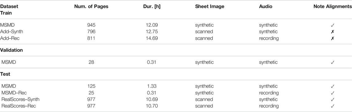
TABLE 3. Overview of datasets used for training, validation and testing.

5.3 Training Details

We train the CYOLO models using the Adam optimizer with corrected weight decay regularization (Loshchilov and Hutter, 2019), a batch size of 128, a learning rate of 5e⁻⁴ that is decreased to 5e⁻⁶ over the course of 50 epochs using cosine annealing (Loshchilov and Hutter, 2017), and a weight decay coefficient of 1e⁻³. Following (He et al., 2019), we apply weight decay only to the weight parameters of convolutional, recurrent and linear layers, but not to normalization layers and bias parameters. Weights are initialized orthogonally (Saxe et al., 2013) and the bias parameters are set to zero except for the forget gate of the LSTM layer which we set to 1 (Gers et al., 2000). In order to avoid exploding gradients, we clip the gradients of the parameters in the recurrent layer of the audio encoder with a maximum norm of 0.1. Model selection for the final evaluation on the test sets is based on the validation loss during training. The baseline models are trained as described in the original references (Dorfer et al., 2016; Henkel et al., 2019, Henkel et al., 2020).

The initial resolution of the used sheet image pages is 1181 × 835, which will be padded to a squared shape and downscaled to 416 × 416 before being presented to the neural network. Visually, this still offers a high enough resolution for humans to distinguish relevant details in the image. For data augmentation the images are randomly shifted along the x and y axis. Additionally, the audio is augmented by changing the tempo with a random factor between 0.5 and 2, and by applying the Impulse Response (IR) augmentation introduced in (Henkel and Widmer, 2021). The latter allows us to model different microphone and room conditions, by convolving the audio recording with a random IR on-the-fly during training. Previous work showed that this results in a more robust audio encoder and significantly improves the tracking accuracy. This augmentation is applied in the same way to all CYOLO models, so that any difference in performance between these will be solely due to whether or not they consider multi-level alignment. That the baseline CYOLO beats the previous models even without this kind of augmentation was already shown in (Henkel and Widmer, 2021).

5.4 Evaluation Metrics

For evaluation we follow (Dixon, 2005; Arzt, 2016) and measure the temporal tracking error of the score following models. Since the predictions of sheet-image-based trackers are positions in an image, we first have to transform them from the spatial domain to the time domain. This is done by using the ground truth alignments between sheet image positions and note onsets, and interpolating from the predicted positions back to the time domain. Subsequently, we compute the absolute time difference between the ground truth and prediction for each note onset. Using this difference, we report the cumulative percentage of notes that are tracked below a certain error threshold, for five threshold values ranging from 0.05 to 5 s.

However, this measure can only be used to evaluate note-level tracking errors. Since we additionally want to evaluate the predicted system and bar alignments of our new approach, we further measure the accuracy based on the intersection over union (IoU) between ground truth and predicted system and bar bounding boxes for each note onset. This is done by using a threshold of 0.8, i. e., a system or bar is considered to be correctly identified if the IoU between the predicted and ground truth bounding box is higher than 0.8.

6 Results and Discussion

In the following we first compare the score following models on the aforementioned datasets to investigate their generalization capabilities. Afterwards, we take a closer look at our best performing model to see under which conditions it still struggles.

6.1 Model Comparison

Table 4 summarizes the results for four different audio and sheet image setups. In the first section (I) we consider the completely synthetic MSMD test split. We observe that the full-page trackers outperform those relying on unrolled scores (MM-Loc and RL) across all error thresholds. Furthermore, CYOLO and its variants all perform similarly and exceed the performance of CUNet. This indicates that predicting system and bar alignments does not hurt the overall performance compared to the plain model, and possibly even improves it since more data can be used.

TABLE 4

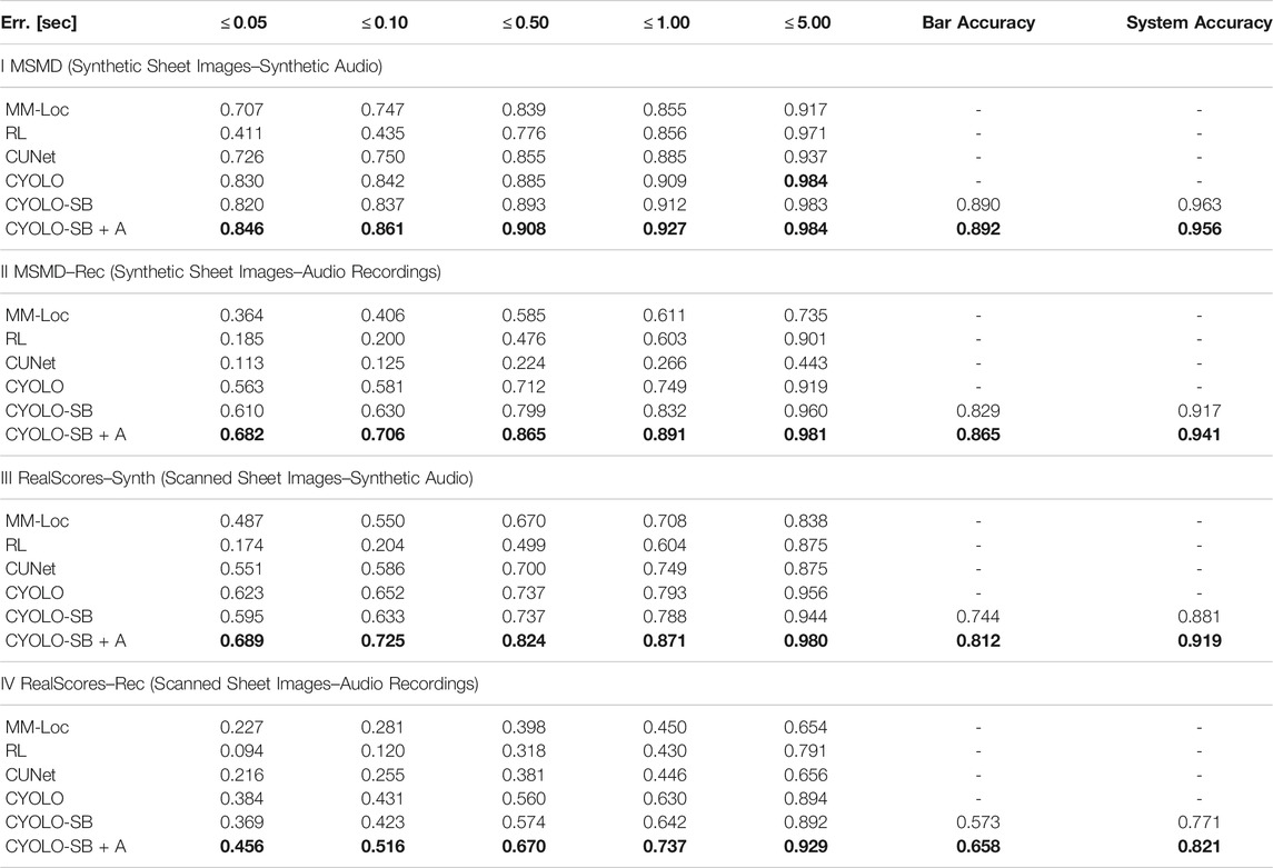
TABLE 4. Comparison of our proposed methods to several approaches on the test sets as described in Section 5. We report the ratio of tracked onsets below certain error thresholds from 0.05 to 5 s. The best result for each threshold is marked bold. Bar and system accuracies are only available for CYOLO-SB and CYOLO-SB + A.⁶

In the second section (II) the performance on the subset of the MSMD test split with real piano recordings is reported. This addresses the question of generalization in the audio domain, without considering different sheet image conditions. Again, we observe that our full-page tracking CYOLO models outperform all other approaches. Interestingly, compared to before, CYOLO-SB outperforms the plain model in this setting. We furthermore see that CYOLO-SB + A improves the results across all error thresholds which is likely due to the additional training data containing several different piano recordings that cannot be used by the other approaches. Moreover, both methods predict the correct bar and system in more than 80% and 90%, respectively.

In the third section (III) we investigate the generalization in the image domain by considering scanned sheet images and synthetic audio, rendered from the score MIDI. While the excerpt-based score following models are lagging behind again, we see that CUNet significantly improved compared to the previous scenario. This indicates that it is better at handling variations in the image than in the audio domain. We further see that CYOLO variants achieve the most precise results, with CYOLO-SB + A performing best. However, we also notice a degradation in terms of the bar and system accuracies compared to synthetic scores.

Finally, in the last section (IV) we report the overall generalization capability of our system by considering both scanned sheet images and piano recordings. As expected, this turns out to be the hardest setting for the score following systems, and we observe a deterioration across all approaches and error metrics. Overall, we see a similar trend compared to the previous setup, where full-page trackers exceed over the excerpt-based ones, and again CYOLO-SB + A performs best. While the additional data leveraged by CYOLO-SB + A could improve the generalization capabilities, there is still a significant gap to the strictly synthetic setting. As we are currently still limited in the amount of data we can use compared to other research areas with an abundance of annotated data (e. g., image classification), we think that collecting a larger (and publicly available) dataset will be key to further improve in this area.

6.2 Error Analysis

In the following, we take a closer look at the average performance of the evaluated methods over all pieces within each dataset. Furthermore, we highlight some examples for which our best performing CYOLO-SB + A model is still struggling.

Figure 7 visualizes the average error distribution across the test datasets. Similar to Table 4, we observe that overall the proposed CYOLO model achieves the lowest alignment error and seems to be more stable accross different pieces. While in some cases the extension with bar and system predictions (CYOLO-SB) is slightly worse than the plain model, CYOLO-SB + A improves upon all other methods. Due to the additional training data, this method achieves the lowest error and the least spread.

FIGURE 7

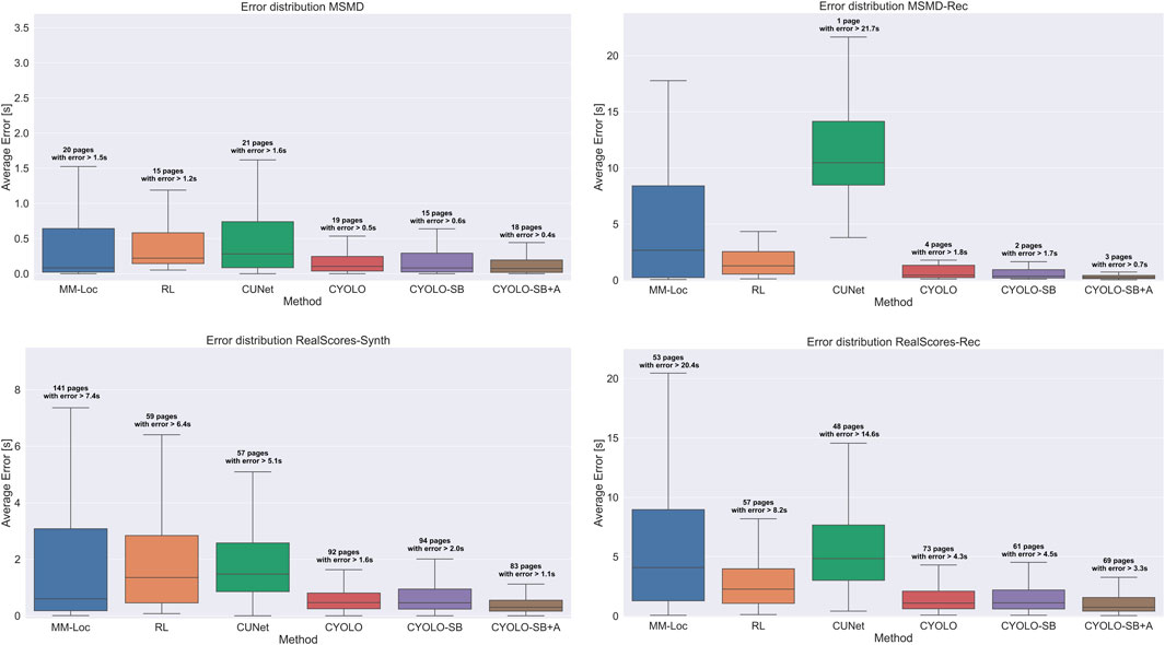
FIGURE 7. Error distributions of compared methods across all test datasets. Outliers are not directly shown (in order not to skew the plots), but given as the number of pages with an error greater than 1.5 × the interquartile range for each method (if there are any).

For the CYOLO-SB + A model we find two particular score pages with a significant error (greater than 3 s) in the test split of the synthetic MSMD dataset. The first one is an extremely slow piece (Catacombae, from Modest Mussorgsky’s Pictures at an Exhibition) consisting almost entirely of dotted half notes, which results in a visually very different score compared to the training pieces and an audio signal with extremely sparse note onsets. For the second piece (Chopin’s Prélude Op. 28, No. 9), we observe two potential pitfalls. On the one hand, the piece contains a few trills, a type of musical ornament where two adjacent notes are played repeatedly in alternation, apparently confusing our system. On the other hand, the piece also has a very repetitive structure, where certain parts only differ by one or two semitones. Given the down-scaled sheet image, it is possibly very hard for the neural network to detect these differences in the image. In future work it will be worth investigating whether a higher input resolution for the sheet image could alleviate such a problem.

For the datasets containing scanned sheet images we observe a larger number of outlier pages. While the average tracking error is in general higher, we again see problems with slower pieces, and pieces containing trills as well as arpeggios, i. e., chords for which each note is played consecutively (cf. Figure 8). It seems that our system struggles to match notes in the performance that are not explicitly marked as separate onsets in the score.

FIGURE 8

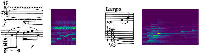
FIGURE 8. Example of a trill (left) and an arpeggio (right), as they look in the score and an audio recording, respectively.

7 Conclusion

In this work we have investigated the generalization capabilities of different sheet-image-based score following approaches. Furthermore, we propose a new method that jointly predicts note-, system-, and bar-level alignments, allowing us to leverage additional data where the annotations are only partially available.

While our approach improved over current state-of-the-art methods, it still lacks a certain level of reliability and robustness, especially in a real-world setup with scanned images and audio recordings. In order to overcome this, we see two important steps to take for future work. First and foremost, we still require more annotated data to train these kinds of score following models. As our new approach allows to use data without fine-grained note-level annotations, it can be easier to collect larger datasets. In particular, it will be important to gather a variety of different sheet images (scanned and possibly also photographed) as well as different audio recordings.

Second, since our current neural network architecture is deliberately kept simple and small compared to state-of-the-art object detection and image classification models (Tan and Le, 2019; Tan et al., 2020; Dosovitskiy et al., 2021), we think there is certainly room for improvement in that direction. The initial bounding box regression problem formulation as well as the newly proposed approach to jointly predict alignments is rather general and not limited to the family of YOLO object detectors. In future work, we want to take a closer look at models such as the Detection Transformer (DETR) (Carion et al., 2020), which gets rid of prior assumptions about bounding box shapes, i. e., anchors, and also offers an alternative conditioning mechanism compared to the FiLM layer we are using. Our new approach could allows us to effectively train such a transformer-based architecture, as these kind of models usually require huge amounts of data.

Data Availability Statement

The data analyzed in this study is subject to the following licenses/restrictions: One part of the training data—the MSMD dataset—is based on prior work and is openly available at https://zenodo.org/record/4745838. The other parts comprise commercial CD recordings and scans of music publishers sheet music that cannot be openly distributed for copyright reasons. As we intend to prove in this paper that our models are robust enough to work on real-world data from the professional world of music, this is unavoidable.

Author Contributions

All authors listed have made a substantial, direct, and intellectual contribution to the work and approved it for publication.

Funding

This work has been supported by the European Research Council (ERC) under the European Union’s Horizon 2020 research and innovation program (grant agreement number 670035, project “Con Espressione”). The LIT AI Lab is funded by the Federal State of Upper Austria.

Conflict of Interest

The authors declare that the research was conducted in the absence of any commercial or financial relationships that could be construed as a potential conflict of interest.

Publisher’s Note

All claims expressed in this article are solely those of the authors and do not necessarily represent those of their affiliated organizations, or those of the publisher, the editors and the reviewers. Any product that may be evaluated in this article, or claim that may be made by its manufacturer, is not guaranteed or endorsed by the publisher.

Footnotes

¹We follow https://github.com/ultralytics/yolov5 for these computations.

²For samples without ground truth note alignments, the objectness loss at the corresponding detection layer is not considered.

³Please note that all CYOLO models are real-time capable. On average (estimated over 100,000 trials), our system takes approx. 6.03 ms to process a new incoming audio frame (corresponding to roughly 50 ms of audio). This is independent of the length of a piece and primarily determined by the duration of a forward path through the neural network (Tested on a system with a consumer GPU (NVIDIA GEFORCE GTX 1080), 32 GB RAM and an Intel i7-7700 CPU).

⁴http://lilypond.org/

⁵https://www.fluidsynth.org

⁶Note that we report a significantly higher performance for MM-Loc compared to previous work. This is due to a bug in the evaluation function that we have fixed for this method

References

Arzt, A. (2016). Flexible and Robust Music Tracking. Ph.D. thesis (Linz: Johannes Kepler University Linz).

Arzt, A., Frostel, H., Gadermaier, T., Gasser, M., Grachten, M., and Widmer, G. (2015). “Artificial Intelligence in the Concertgebouw,” in Proceedings of the 24th International Joint Conference on Artificial Intelligence (IJCAI), 2424–2430.

Google Scholar

Arzt, A., Widmer, G., and Dixon, S. (2008). “Automatic Page Turning for Musicians via Real-Time Machine Listening,” in Proceedings of the 18th European Conference on Artificial Intelligence (ECAI), 241–245.

Google Scholar

Ba, J. L., Kiros, J. R., and Hinton, G. E. (2016). Layer Normalization. arXiv preprint arXiv:1607.06450.

Google Scholar

Bochkovskiy, A., Wang, C.-Y., and Liao, H.-Y. M. (2020). YOLOv4: Optimal Speed and Accuracy of Object Detection. arXiv preprint arXiv:2004.10934.

Google Scholar

Calvo-Zaragoza, J., Hajič, J., and Pacha, A. (2019). Understanding Optical Music Recognition. New York: Computer Research Repository. abs/1908.03608.

Google Scholar

Cancino-Chacón, C., Bonev, M., Durand, A., Grachten, M., Arzt, A., Bishop, L., et al. (2017a). “The ACCompanion V0. 1: An Expressive Accompaniment System,” in Late Breaking/Demo, 18th International Society for Music Information Retrieval Conference (ISMIR).

Google Scholar

Cancino-Chacón, C. E., Gadermaier, T., Widmer, G., and Grachten, M. (2017b). An Evaluation of Linear and Non-linear Models of Expressive Dynamics in Classical Piano and Symphonic Music. Mach Learn. 106, 887–909. doi:10.1007/s10994-017-5631-y

CrossRef Full Text | Google Scholar

Carion, N., Massa, F., Synnaeve, G., Usunier, N., Kirillov, A., and Zagoruyko, S. (2020). “End-to-End Object Detection with Transformers,” in European Conference on Computer Vision (ECCV) (Springer), 213–229. doi:10.1007/978-3-030-58452-8_13

CrossRef Full Text | Google Scholar

Clevert, D., Unterthiner, T., and Hochreiter, S. (2016). “Fast and Accurate Deep Network Learning by Exponential Linear Units (ELUs),” in Proceedings of the 4th International Conference on Learning Representations (ICLR).

Google Scholar

Cont, A. (2010). A Coupled Duration-Focused Architecture for Real-Time Music-To-Score Alignment. IEEE Trans. Pattern Anal. Mach. Intell. 32, 974–987. doi:10.1109/tpami.2009.106

PubMed Abstract | CrossRef Full Text | Google Scholar

Cont, A. (2006). “Realtime Audio to Score Alignment for Polyphonic Music Instruments Using Sparse Non-negative Constraints and Hierarchical HMMS,” in Proceedings of the IEEE International Conference on Acoustics, Speech, and Signal Processing (ICASSP), 245–248.

Google Scholar

Dixon, S. (2005). “An On-Line Time Warping Algorithm for Tracking Musical Performances,” in Proceedings of the 19th International Joint Conference on Artificial Intelligence (IJCAI), 1727–1728.

Google Scholar

Dorfer, M., Arzt, A., and Widmer, G. (2016). “Towards Score Following in Sheet Music Images,” in Proceedings of the 17th International Society for Music Information Retrieval Conference (ISMIR), 789–795.

Google Scholar

Dorfer, M., Hajič, J., Arzt, A., Frostel, H., and Widmer, G. (2018a). Learning Audio–Sheet Music Correspondences for Cross-Modal Retrieval and Piece Identification. Trans. Int. Soc. Music Inf. Retrieval 1, 22. doi:10.5334/tismir.12

CrossRef Full Text | Google Scholar

Dorfer, M., Henkel, F., and Widmer, G. (2018b). “Learning to Listen, Read, and Follow: Score Following as a Reinforcement Learning Game,” in Proceedings of the 19th International Society for Music Information Retrieval Conference (ISMIR), 784–791.

Google Scholar

Dosovitskiy, A., Beyer, L., Kolesnikov, A., Weissenborn, D., Zhai, X., Unterthiner, T., et al. (2021). “An Image Is Worth 16x16 Words: Transformers for Image Recognition at Scale,” in Proceedings of the 9th International Conference on Learning Representations (ICLR).

Google Scholar

Flossmann, S., Goebl, W., Grachten, M., Niedermayer, B., and Widmer, G. (2010). The Magaloff Project: An Interim Report. J. New Music Res. 39, 363–377. doi:10.1080/09298215.2010.523469

CrossRef Full Text | Google Scholar

Gers, F. A., Schmidhuber, J., and Cummins, F. (2000). Learning to Forget: Continual Prediction with LSTM. Neural Comput. 12, 2451–2471. doi:10.1162/089976600300015015

PubMed Abstract | CrossRef Full Text | Google Scholar

Grill, T., and Schlüter, J. (2017). “Two Convolutional Neural Networks for Bird Detection in Audio Signals,” in Proceedings of the 25th European Signal Processing Conference (EUSIPCO), 1764–1768. doi:10.23919/eusipco.2017.8081512

CrossRef Full Text | Google Scholar

He, T., Zhang, Z., Zhang, H., Zhang, Z., Xie, J., and Li, M. (2019). “Bag of Tricks for Image Classification with Convolutional Neural Networks,” in Proceedings of the IEEE/CVF Conference on Computer Vision and Pattern Recognition (CVPR), 558–567. doi:10.1109/cvpr.2019.00065

CrossRef Full Text | Google Scholar

Henkel, F., Balke, S., Dorfer, M., and Widmer, G. (2019). Score Following as a Multi-Modal Reinforcement Learning Problem. Trans. Int. Soc. Music Inf. Retrieval 2. doi:10.5334/tismir.31

CrossRef Full Text | Google Scholar

Henkel, F., Kelz, R., and Widmer, G. (2020). “Learning to Read and Follow Music in Complete Score Sheet Images,” in Proceedings of the 21st International Society for Music Information Retrieval Conference (ISMIR), 780–787.

Google Scholar

Henkel, F., and Widmer, G. (2021). “Multi-modal Conditional Bounding Box Regression for Music Score Following,” in Proceedings of the 29th European Signal Processing Conference (EUSIPCO).

Google Scholar

Hochreiter, S., and Schmidhuber, J. (1997). Long Short-Term Memory. Neural Comput. 9, 1735–1780. doi:10.1162/neco.1997.9.8.1735

PubMed Abstract | CrossRef Full Text | Google Scholar

Hu, R., Rohrbach, M., and Darrell, T. (2016). “Segmentation from Natural Language Expressions,” in Proceedings of the 14th European Conference on Computer Vision (ECCV), 108–124. doi:10.1007/978-3-319-46448-0_7

CrossRef Full Text | Google Scholar

Ioffe, S., and Szegedy, C. (2015). “Batch Normalization: Accelerating Deep Network Training by Reducing Internal Covariate Shift,” in Proceedings of the 32nd Int. Conference on Machine Learning (ICML), 448–456.

Google Scholar

Loshchilov, I., and Hutter, F. (2019). “Decoupled Weight Decay Regularization,” in Proceedings of the 7th International Conference on Learning Representations (ICLR).

Google Scholar

Loshchilov, I., and Hutter, F. (2017). “SGDR: Stochastic Gradient Descent with Warm Restarts,” in Proceedings of the 5th International Conference on Learning Representations (ICLR).

Google Scholar

Nakamura, E., Cuvillier, P., Cont, A., Ono, N., and Sagayama, S. (2015). “Autoregressive Hidden Semi-markov Model of Symbolic Music for Score Following,” in Proceedings of the 16th International Society for Music Information Retrieval Conference (ISMIR), 392–398.

Google Scholar

Orio, N., Lemouton, S., and Schwarz, D. (2003). “Score Following: State of the Art and New Developments,” in Proceedings of the International Conference on New Interfaces for Musical Expression (NIME), 36–41.

Google Scholar

Perez, E., Strub, F., De Vries, H., Dumoulin, V., and Courville, A. (2018). “FiLM: Visual Reasoning with a General Conditioning Layer,” in Proceedings of the 32nd AAAI Conference on Artificial Intelligence, 3942–3951.

Google Scholar

Raphael, C. (2010). “Music Plus One and Machine Learning,” in Proceedings of the International Conference on Machine Learning (ICML), 21–28.

Google Scholar

Redmon, J., Divvala, S., Girshick, R., and Farhadi, A. (2016). “You Only Look once: Unified, Real-Time Object Detection,” in Proceedings of the IEEE Conference on Computer Vision and Pattern Recognition (CVPR), 779–788. doi:10.1109/cvpr.2016.91

CrossRef Full Text | Google Scholar

Redmon, J., and Farhadi, A. (2017). “YOLO9000: Better, Faster, Stronger,” in Proceedings of the IEEE Conference on Computer Vision and Pattern Recognition (CVPR), 6517–6525. doi:10.1109/cvpr.2017.690

CrossRef Full Text | Google Scholar

Ridnik, T., Lawen, H., Noy, A., and Friedman, I. (2020). TResNet: High Performance GPU-Dedicated Architecture. arXiv preprint arXiv:2003.13630

Google Scholar

Saxe, A. M., McClelland, J. L., and Ganguli, S. (2013). Exact Solutions to the Nonlinear Dynamics of Learning in Deep Linear Neural Networks. arXiv preprint arXiv:1312.6120.

Google Scholar

Shan, M., and Tsai, T. (2020). “Improved Handling of Repeats and Jumps in Audio-Sheet Image Synchronization,” in Proceedings of the 21st International Society for Music Information Retrieval Conference (ISMIR), 62–69.

Google Scholar

Tan, M., and Le, Q. V. (2019). “Efficientnet: Rethinking Model Scaling for Convolutional Neural Networks,” in International Conference on Machine Learning (ICML) (PMLR), 6105–6114.

Google Scholar

Tan, M., Pang, R., and Le, Q. V. (2020). “EfficientDet: Scalable and Efficient Object Detection,” in Proceedings of the IEEE/CVF conference on Computer Vision and Pattern Recognition (CVPR), 10781–10790. doi:10.1109/cvpr42600.2020.01079

CrossRef Full Text | Google Scholar

Tanprasert, T., Jenrungrot, T., Müller, M., and Tsai, T. (2019). “Midi-Sheet Music Alignment Using Bootleg Score Synthesis,” in Proceedings of the 20th International Society for Music Information Retrieval Conference (ISMIR), 91–98.

Google Scholar