The Eastern Mediterranean Sea mean sea level decadal slowdown: the effects of the water budget

This paper analyses the decadal variability of the Mean Sea Level (MSL) trend for the Mediterranean Sea and three subregions using a combination of satellite altimetry, tide gauges and reanalyses datasets for the past 30 years (1993–2022). These estimates indicate a decadal variability of the MSL across the analysed period, and a trend slowdown in the 2013–2022 decade compared to previous periods. While the overall trend remains positive across the Mediterranean basin, regional differences are evident. The Western Mediterranean shows an accelerating trend, consistent with global sea level rise, while the Eastern Mediterranean has experienced a decadal slowdown, particularly in the semi-enclosed Adriatic and Aegean Seas, where negative trends are observed. This slowdown is attributed to the combined effects of changes in the water cycle and the balancing of thermal and haline steric components. A key driver of this trend is increased evaporation, which is not offset by precipitation, runoff, or transport through the Straits. These results underscore the significance of the Mediterranean’s water budget in influencing sea level trends and highlight the complexity of modelling and interpreting decadal sea level changes. The findings suggest that continued monitoring and a better understanding of regional water budgets are crucial for refining future projections and developing effective climate adaptation strategies for the Mediterranean coastal areas.

1 Introduction

The Global Mean Sea Level (GMSL) has been extensively analysed over the past decades as a key indicator of the impact of climate change on coastal regions (IPCC, 2023). Numerous studies confirm a positive GMSL trend over the last century, estimated at 1.6 ± 0.4 mm/year (Hay et al., 2015), with evidence pointing to an acceleration over the last 30 years (Ablain et al., 2019; Dangendorf et al., 2019; Merrifield et al., 2009). However, regional Mean Sea Level (MSL) can be affected by large temporal variability in the ocean circulation and buoyancy forcings, thus influencing the trend from interannual to decadal time scales (Moreira et al., 2021; Stammer et al., 2013). As a result, regional trends can substantially deviate from the GMSL values, making precise local estimates crucial for developing management solutions.

This is particularly relevant for the Mediterranean Sea, where a positive Mediterranean MSL (MMSL) trend of 2.1 ± 0.5 mm/year was observed between 1993 and 2019 (Meli et al., 2023), differing from the GMSL trend of 3.3 ± 0.3 mm/year approximately during the same period (Guérou et al., 2023). Indeed, a negative surface buoyancy flux over the basin forces an anti-estuarine circulation across the Gibraltar Strait (Cessi et al., 2014), and the complex geometry (Figure 1) results in a specific upper ocean circulation of different water masses throughout the entire region (Pinardi et al., 2015, 2019). The resulting circulation structures impact the variability of both mass and steric components of the sea level, as documented for the negative sea level trend in the Ionian Sea during the 1990s, attributed to the Northern Ionian Gyre (Bonaduce et al., 2016; Criado-Aldeanueva et al., 2008; Meli, 2024).

Figure 1

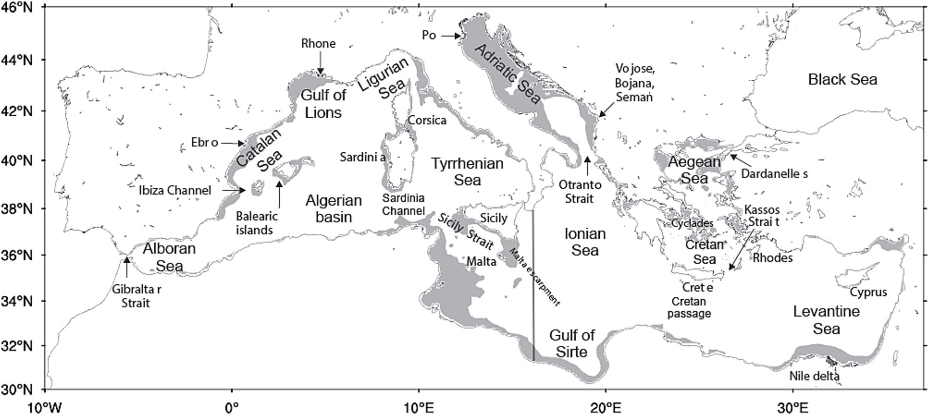
Figure 1. Mediterranean Sea basin geometry and nomenclature for major seas and areas. The shaded areas indicate depths less than 200 m. The thin black line corresponds to the meridional transect used to define the western boundary of Eastern Mediterranean Sea at 16°E.

We started our investigation of the sea level trends for the Adriatic Sea, being part of a project that was discussing the future climate projections of this area (da Costa et al., 2024; Verri et al., 2024). The results indicated a decrease of the sea level trend in the historical period and in the future projections and we wanted to add more analysis from observations to these results. Upon expanding our analysis to the Eastern Mediterranean, we identified that the observed slowdown was part of a broader pattern of change affecting also other areas, such as the Aegean Sea. Thus, our study will focus on observations and on Western, Eastern and Adriatic Sea sub-basins.

With 30 years of satellite sea level data and regional reanalysis datasets now available, it is possible to analyse the differences between long-term and decadal MSL trends. Notably, the World Meteorological Organization (2024) documented that the decadal rate of GMSL rise has more than doubled since the beginning of the satellite era, increasing from 2.13 mm/year in the 1993–2002 period to 4.77 mm/year between 2014 and 2023. Furthermore, Cazenave et al. (2014) documented a decadal slowdown for the GMSL due to interannual variability in the global water cycle. Using the same approach applied to the Mediterranean Sea, we quantify the decadal and multidecadal trends of the MMSL and distinguish subregional patterns.

Given the observational evidence, this work aims to show the decadal variability of the MSL trends and their variability across the Mediterranean basin, as well as the contributing factors to it. On a global scale, the causes of sea-level rise are primarily attributed to the melting of land ice, which contributes to the sea-level mass component, and the thermal expansion of ocean water, which affects the steric component (accounting for 80 and 20% of the observed variation, respectively, according to Milne et al., 2009).

Calafat et al. (2012) were the first to demonstrate that the steric components of the Mediterranean Sea level can account for at most 30% of the total sea level, in contrast to the North Atlantic, where this contribution exceeds 80%. Pinardi et al. (2014) showed that the Mediterranean Sea’s mass component introduces a significant stochastic-like term that varies at interannual timescales. Meli et al. (2023) found that thermal expansion and salinity contraction offset each other in the steric contribution to sea level in the Mediterranean Sea. Consequently, all these studies conclude that the mass component is essential for understanding sea level trends.

Recently, García-García et al. (2022) revisited the Mediterranean water balance for a shorter period (2002–2020), which only partially covers the observational satellite data set period and does not link the water budget components to sea level trends. Verri et al. (2024) analyzed the impact of decreased river runoff on the MSL trend in the Northern Adriatic Sea, highlighting the significance of such changes in mitigating sea level rise due to thermal expansion effects. However, neither study calculates the decadal mass balance changes over the past 30 years of the satellite altimetry period, nor do they connect the observed sea level trends with the magnitude and variations of water mass and steric terms. In this paper, we analyze the decadal changes in the mass and steric components contributing to MSL in the Mediterranean and Eastern Mediterranean Seas, with the aim to quantify the water balance contribution to the observed MSL trends. We propose that decadal trends are just as important as multidecadal trends, as they may lead to distinct hazards and impacts. For example, the effects of sea level rise —whether linear or accelerated— can vary significantly in terms of coastal erosion and eutrophication because compound impacts are influenced by the timescales over which interacting signals occur.

In section 2 we explain datasets used and the pre-processing carried out to compute decadal mean sea level trend. In section 3 we compute the decadal sea level trends in different subregions of the Mediterranean Sea, verify the contribution of the sea level steric component, and analyse the importance of combined surface water budget changes and mass transport on the open boundaries of the basin. In section 4 the results are discussed in the framework of global and regional climate adaptation strategies, and finally section 5 concludes the paper.

2 Data and methods

2.1 Observational datasets

The evolution of observed sea level in the Mediterranean Sea is analysed over the past 30 years by examining satellite and in-situ observations.

Altimetric datasets are used to investigate different regions of the Mediterranean (Figure 1). Altimeter satellite gridded Sea Level Anomalies (SLA) are analysed using two different datasets provided by the Copernicus Marine Service catalogue. The first product is the European seas gridded L4 sea surface height, hereafter referred to as CMS (European Seas Gridded L 4 Sea Surface Heights and Derived Variables Reprocessed 1993 Ongoing, n.d.). It contains SLA from January 1993 to December 2022, computed with respect to a 20-year (1993–2012) mean sea surface height over the European seas at 1/8° of resolution and daily frequency. CMS focuses on the mesoscale mapping of the sea level, merging along-track altimetry data from all available missions (TOPEX-Poseidon, ERS, Jason-X, Altika, ENVISAT, Sentinel-3, 6 and Cryosat).

Given that each satellite is characterized by different sampling errors, the use of a varying number of satellites could introduce a bias in SLA tendencies. To address this, a second dataset is considered, the gridded SLA from the Copernicus Climate Change service, hereafter referred to as C3S (Global Ocean Gridded L4 Sea Surface Heights and Derived Variables Reprocessed Copernicus Climate Service, n.d.). This dataset is specifically designed to ensure the homogeneity and stability of the global and regional sampling rate in the past 30 years. It uses only the reference missions (TOPEX-Poseidon, Jason-1, Jason-2 and Jason-3, Sentinel-6A) which have same repeat orbits of 10 days, and they overlap for some years. It provides data with a spatial resolution of 1/4° for the same period as CMS and the same daily frequency.

The two datasets use different methods to compute the SLA, although they refer to the same reference period (2003–2012): CMS uses a mean profile of sea surface height along the altimeter tracks for each satellite mission, whereas C3S uses the same mean sea surface for all missions. Both datasets use tidal corrections to eliminate the tidal components of sea level. In both cases, a limitation in SLA data accuracy arises from the optimal interpolation algorithm applied to along-track data to map on a uniform spatial and temporal grid (Chelton and Schlax, 2003). In Chelton and Schlax (2003) it is stated that the best accuracy in the mapped SLA is achieved when only two satellites with interleaving tracks are used, that is the case of the C3S dataset. Both CMS and C3S are corrected to remove the TOPEX-A instrumental drift from 1993 to 1998, derived from altimetry and tide gauge global comparisons (WCRP Global Sea Level Budget Group, 2018). Even though this is a global mean correction, it can be applied at regional scale as a best estimate, due to the lack of information on regional variations in the instrumental drift (Watson et al., 2015).

Focusing on the specific region of the Eastern Mediterranean, the sea level trend computed from satellites is compared with in-situ observations in Hadera, Venice and Trieste, where tide gauges data are available from the Permanent Service of Mean Sea Level (PSMSL) database (Holgate et al., 2012). The dataset provides information of monthly mean sea level timeseries. The stations are selected by seeking a compromise between optimal regional coverage and the presence of missing data in the time series. When gaps are present, the timeseries are analysed without applying any filling-the-gap interpolation. These data are also used to validate the satellite SLA in the Adriatic and Levantine Seas. A correlation is computed by comparing de-seasoned in-situ tide gauges with the corresponding nearest points from the de-seasoned CMS and C3S satellite datasets. Given the different temporal resolutions, satellite data are first averaged in time to obtain monthly time series. For the CMS dataset, the correlation values are 0.77 in Trieste, 0.81 in Venice, and 0.84 in Hadera (similar values for the C3S dataset are reported in the Supplementary material, along with the overlapping time series).

2.2 Reanalysis datasets

The Mediterranean Sea high resolution ocean reanalysis by Escudier et al. (2021), hereafter referred to as MEDREA24, is used to determine the sea level steric component and the long-term evolution of the mass transport at the Gibraltar Strait at 5.5°W and across the Calabrian section at 16°E. There are many studies of water transport at Gibraltar (García-García et al., 2022; Jordà et al., 2017) but none of them attempted to estimate trends for the 30-year period of the satellite sea level data. The MEDREA24 general circulation model is based on the Nucleus for European Modelling of the Ocean, NEMO (Madec et al., 2017). The model has a horizontal resolution of 1/24° (~ 4 km), and 141 unevenly distributed vertical levels in the z^* coordinate system (Adcroft and Campin, 2004). Atmospheric hourly fields from ERA5 reanalysis (Hersbach et al., 2020) are used in bulk formulae to force the model by momentum, water and heat fluxes, while the daily boundary conditions in the Atlantic are taken from a global reanalysis. The SST satellite data is used to correct the heat fluxes and all in-situ data, from CTD (ship measurements of Conductivity Temperature and Depth), ARGO floats and XBT (Expendable BathyThermograph) are assimilated into the model in combination with satellite altimetry observations using the OceanVar data assimilation scheme (Dobricic and Pinardi, 2008).

Data on evaporation and precipitation are obtained from ERA5 atmospheric reanalysis (Hersbach et al., 2020), at a spatial resolution of 1/4° over the Mediterranean Sea and monthly frequency. Considering the different evaporation processes affecting sea and land surfaces, as well as the significant uncertainty associated with precipitation estimates over the sea (Stocchi and Davolio, 2017), we focus on grid points where more than 50% of the area is covered by sea.

Finally, data on river discharges are retrieved from the European Flood Awareness System (EFAS). The EFAS v5.0 hydrological reanalysis dataset is extracted from the Copernicus Emergency Management Service (Smith et al., 2016) that contains two-dimensional discharges (in m³/s) at the horizontal resolution of ~1.5 km and 6-hourly frequency. The Local Drain Direction (LDD) expresses the flow direction from one cell to another in the hydrological model, forming a river network from the springs to the mouth. In this study, we calculate river runoff as the sum of discharges across all grid points defined as outflow grid cells for the LDD along the coastlines. Additionally, we excluded the outflow grid points along the Libyan and Egyptian coasts, except for the Nile delta, as there is no evidence of other rivers in this area besides the Nile.

2.3 Analysis methods

To compute the MSL decadal and multidecadal trends from CMS and C3S in the 1993–2022 period, data are first averaged over the regions of interest, that are the entire Mediterranean Sea, its Western and Eastern subbasins (MED, WMED and EMED hereafter), and the Adriatic Sea. Based on the trend patterns (described in section 3.1), the boundary between WMED and EMED is defined along the meridional transect at 16°E (Figure 1).

From the regionally averaged SLA time series, the daily seasonal cycle is computed and then subtracted to obtain the non-seasonal SLA (NS-SLA). Figure 2 shows that, at the basin scale, the maximum difference between the C3S and CMS estimated seasonal cycle is 1 cm, particularly in the autumn and winter seasons, due to mesoscale-driven effects differently resolved by the two datasets. The seasonal cycle amplitude is approximately 16 cm, as documented in several studies (Adani et al., 2011; Bonaduce et al., 2016).

Figure 2

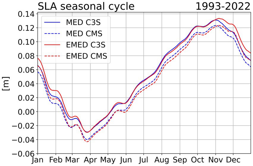
Figure 2. The 1993–2022 basin average and time mean daily seasonal cycle of SLA computed from the original timeseries in the MED and EMED domains: C3S dataset (solid lines) and CMS dataset (dashed lines).

The NS-SLA represents a combination of interannual variability and higher-frequency components such as multi-year gyres and yearly variability. To effectively separate long-term trends from short-term fluctuations, we apply a low-pass filter to the timeseries, removing frequencies above 5 cycles/year. The transition band is smoothed using a Tukey window to ensure a gradual adjustment, and we refer to Alessandri et al. (2023) for a more detailed description of the filtering procedure.

Following the analysis proposed by Cazenave et al. (2014), decadal linear trends are evaluated over the 1993–2022 period, here decomposed over 10-year-long sliding windows shifted by 1 year. A 10-year interval is considered the minimum time needed to compute trends over the entire domain of interest, accounting for the uncertainty associated with SLA annual mean values without loss of accuracy, in accordance with Montgomery and Runger (2018).

The trends are estimated using the Theil-Sen slope (Sen, 1968; Theil, 1992), a robust and interpretable method for quantifying trend magnitude. This approach is less sensitive to outliers compared to traditional linear regression, providing reliable estimates even in the presence of data variability. The statistical significance of the trends is assessed using the Mann-Kendall test (Kendall, 1948; Mann, 1945), modified for autocorrelated data following the methodology of Hamed and Ramachandra Rao (1998). A trend is deemed statistically significant for p-values below 0.05, corresponding to a 95% confidence level and higher.

For the three non-overlapping decades (1993–2002, 2003–2012, 2013–2022), we employ a robust statistical analysis to assess the significance of the observed trend variations. The procedure involves the following steps:

1. The determination of a trend-residual time series obtained by subtracting the trend previously calculated from the low-pass filtered data.

2. From the trend-residual timeseries, we generate a distribution of possible residuals by applying the stationary bootstrap scheme (Politis and Romano, 1994) with 5,000 iterations, selecting an optimal block length based on the method proposed by Patton et al. (2009).

3. The linear fit trend is then re-added to reconstruct 5,000 full NS-SLA time series with differently distributed residuals. Next, the Theil-Sen slope is computed for each reconstructed time series, yielding a statistical distribution of possible NS-SLA trends for the period of interest. The mean of this distribution represents the final NS-SLA trend, while its standard deviation provides an estimate of the associated uncertainty.

Lastly, Welch’s t-test (Welch, 1947) is used to evaluate the statistical significance of trend differences between decades, enabling a robust comparison of trend variations. Decadal trend values are also computed at each grid point of the satellite datasets to evaluate their spatial distribution. Specifically, the linear regression method is applied to the NS-SLA timeseries to estimate both the trend values and their statistical significance.

For the tide gauge stations listed in section 2.1, the original monthly data are first pre-processed to remove the seasonal cycle, neglecting missing values, to obtain the de-seasoned monthly mean sea level. Then, the sea level decadal and multidecadal trends are computed using the linear regression method. The error associated to trend estimate is computed as the standard error between the linear fit and the yearly mean sea level values, under the assumption of residual normality.

Reanalysis atmospheric and oceanic datasets are analysed to compare the MSL equation terms on decadal time scales (1993–2002, 2003–2012 and 2013–2022) and over the entire 30-year period. Thus, the decadal mean values of evaporation, precipitation, river runoff and lateral transport at the open boundaries of the domain are computed for the MED and EMED regions. As in the NS-SLA trend case, the errors associated to each value are evaluated using the stationary bootstrap scheme proposed by Politis and Romano (1994), selecting an optimal block length according to Patton et al. (2009).

3 Results

3.1 Decadal Mediterranean mean sea level trends

Figure 3 shows the decadal trends for each grid point in the CMS and C3S products. Despite their different resolutions and purposes, both products exhibit the same behaviour. The decadal maps highlight the geographical distribution of the sea level rise and fall (Bonaduce et al., 2016; Mohamed et al., 2019), emphasizing the limitations associated with multi-decadal trends (as reported by Vigo et al., 2005). In the maps the points with below the 95% confidence interval are shown. The trend values are statistically significant over almost all areas, except in regions where the trend is close to zero and changes sign.

Figure 3

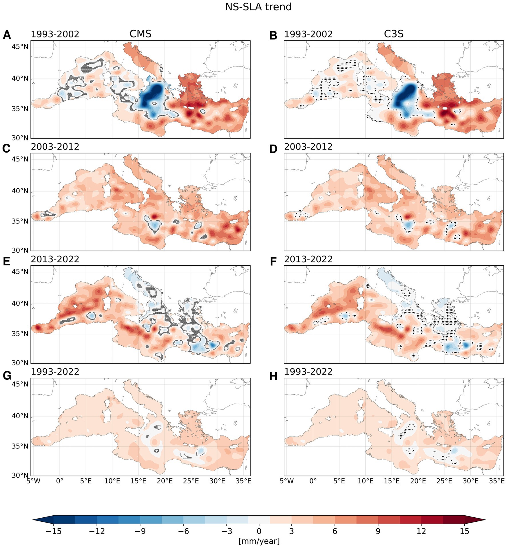
Figure 3. Maps of NS-SLA trend from CMS (left) and C3S (right) datasets. The periods of estimated trend are: 1993–2002 (A,B), 2003–2012 (C,D), 2013–2022 (E,F), and 1993–2022 (G,H). The black dots indicate points where the p-values are larger than 0.05, so the trend estimation has no statistical significance.

In the first decade, between 1993 and 2002, the NS-SLA trend is strongly heterogeneous (Figures 3A,B). The western basin shows weakly positive trends in the Alboran and Algerian Seas, and nearly null trends in the Balearic and Southern Tyrrhenian Seas. Conversely, the eastern basin exhibits large positive and negative trends. In particular, the highest positive trends are detected in the Cretan Passage and Aegean Sea, while a negative trend is observed in the Ionian Sea, attributed to the well-documented North Ionian Gyre (NIG) reversal during the 1990s (Bonaduce et al., 2016; Criado-Aldeanueva et al., 2008; Meli, 2024).

In the second decade, from 2003 to 2012, the NS-SLA trends become more uniform across the MED, with regional patches of larger trend values in the Southern Ionian and Levantine Seas (Figures 3C,D). During this period, the NS-SLA decreases in limited areas offshore the Gulf of Sirte and southeast of Crete, possibly related to the evolution of mesoscale structures like the long-lived Ierapetra eddy (Ioannou et al., 2017). This decade appears to act as a transition period between two different subbasin regimes.

Indeed, during the last decade from 2013 to 2022, the observed NS-SLA trend behaves oppositely compared to the first period (Figures 3E,F). Higher trends are reported in the Western Mediterranean and the Sicily Strait, while weakly positive or negative trends are found in the Eastern Mediterranean. In CMS, the western side is characterised by an average trend of 4 mm/year, while the eastern side by 1 mm/year. The overall inversion of the trend sign from the first to the third decade is particularly notable in the semi-enclosed Aegean and Adriatic Seas (more details in section 3.1.1) and in the Southern Levantine Sea (Vigo et al., 2005).

Over the course of 30 years, the evolution of the sea level trend has therefore reversed between the western and eastern regions of the Mediterranean Sea. As expected, the trend over the entire analysed period (Figures 3G,H) smooths out the multiannual variability observed in the sub-basins, showing NS-SLA rise ranging from 1.5 to 4.5 mm/year almost everywhere, except a statistically non-significant signal in the Ionian Sea and the Cretan Passage. The decadal trend provides a novel description of the evolution of sea level: in the last decade, the sea level trend is rising in the western portion of the basin and slowing down in the eastern counterpart, with specific regions where this phenomenon is more intense.

The sea level evolution of the MED can furthermore be represented by averaging the NS-SLA timeseries over selected regions of interest. Based on the trend distribution over the three decades (Figure 3), the boundary between WMED and EMED is defined along the Calabrian section at 16°E. Figure 4 shows the timeseries of the entire MED, while those separately for EMED and WMED are reported in the Supplementary material.

Figure 4

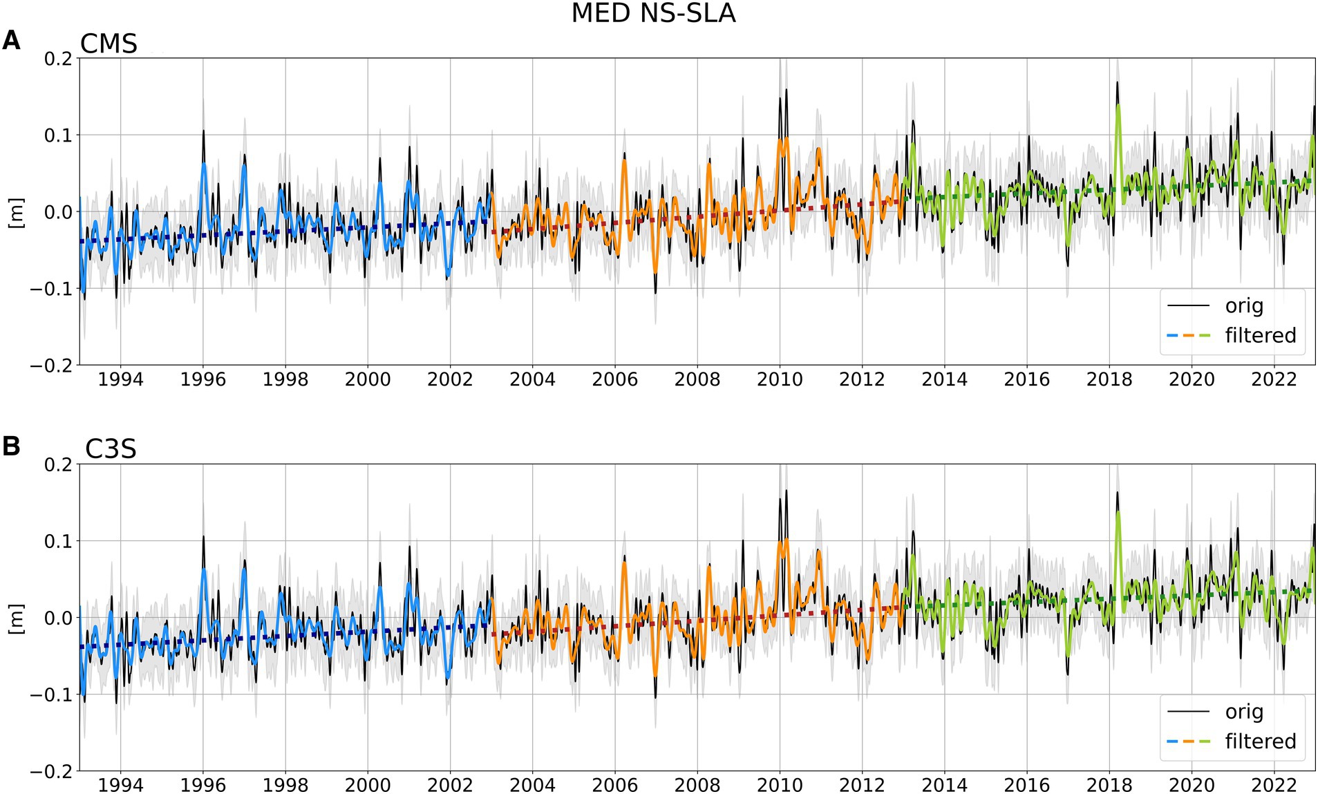
Figure 4. Timeseries of daily NS-SLA in the MED from CMS (A) and C3S (B) during the period 1993–2022. The original timeseries is shown in black, with the grey shaded area indicating the associated uncertainty. The low-pass filtered timeseries is also shown, with each decade represented by a different colour: 1993–2002 (blue), 2003–2012 (orange) and 2013–2022 (green). The linear fits for each decade are shown as dotted lines. Values of decadal and multidecadal trends are reported in Table 1.

From Figure 4 it is evident that the different decadal trends are due to interannual variability peaks that last almost 1 year and that are large amplitude. This is something that was found also by Cazenave et al. (2014) for the GMSL slowdown on the 2000–2010 decade and we show here that something similar is occurring in the MED but for different decades. Furthermore, the decadal slowdown is larger for the EMED (Supplementary material).

The NS-SLA trends are summarised in Table 1 for the periods 1993–2002, 2003–2012, 2013–2022 and 1993–2022, and the correspondent t-test values are reported in the Supplementary material. Examining the 30-year trend from CMS and C3S, the MMSL trend attains a positive value of 2.6 ± 0.2 mm/year and 2.4 ± 0.2 mm/year, respectively. These values align with the value of 2.5 ± 0.83 mm/year proposed by the Copernicus Marine Service (Mediterranean Sea Mean Sea Level time series and trend from Observations Reprocessing, n.d.). Trends are slightly higher when computed for the period 2006–2018 (3.2 ± 1.0 mm/year in CMS, and 2.6 ± 1.1 mm/year in C3S), but are still lower compared to the global mean of 3.7 ± 0.5 mm/year for the same period (IPCC, 2023).

Table 1

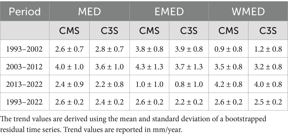
Table 1. Decadal and multidecadal trends of MSL in the MED, EMED, and WMED, computed from daily time series of low-pass filtered NS-SLA from CMS and C3S datasets.

Focusing on trends computed over non-overlapping decades, the first and third periods show positive values consistent with the long-term behaviour, while the second decade reports a stronger sea level rise (4.0 ± 1.0 mm/year in CMS, and 3.6 ± 1.0 mm/year in C3S). According to Figure 3, the increased MMSL trend from the first to the second decade is misleading, as between 2003 and 2012 this larger value is due to the changes in the Ionian Sea, where the negative trend associated with the NIG reversal disappears. The trend difference between the second and the third decades clearly shows a general slowdown of the sea level trend over the EMED, while the sea level is accelerating in the WMED. The slowdown observed in the eastern side of the domain has a greater impact than the acceleration seen in the western counterpart, leading to an overall slowdown of the MMSL trend over the period 2013–2022.

The EMED MSL (EM-MSL) trend is then the main driver of the observed variations over the entire basin. According to Table 1, the trend computed from CMS in the EMED changes from 3.8 ± 0.8 mm/year (1993–2002) to 4.3 ± 1.3 mm/year (2003–2012), and finally drops to 1.0 ± 1.0 mm/year in the last decade. Conversely, the WMED trend increases from 0.9 ± 0.8 mm/year (1993–2002) to 3.5 ± 0.8 mm/year (2003–2012) and 4.2 ± 0.8 mm/year (2013–2022).

It is worth noting a remarkable difference between CMS and C3S during the 2003–2012 period in the EMED: although the two trend values are comparable within the estimated uncertainty, they lead to different interpretations. According to CMS, the trend increased from the first to the second period. On the contrary, C3S indicates that the trend slowdown began during the second decade, with the value decreasing from 3.9 ± 0.8 mm/year to 3.7 ± 1.3 mm/year. This discrepancy can be probably attributed to the differences in the basic satellite datasets used to produce the CMS and C3S products.

To avoid the potential limitations associated to the specific choice of three specific time intervals, we calculate the MSL decadal trend for sliding time windows across the 1993–2022 period.

Looking at the entire basin (Figure 5A), the CMS decadal trend is statistically significant throughout the 30-year period, with the only exception being the period centered around 2001 (corresponding to the decade 1996–2005), when the sea level trend is nearly flat. In the WMED (Figure 5B), the trend is negligible in the early period, but then increases almost monotonically, which aligns with the behavior observed in the global ocean (Dangendorf et al., 2019). In the EMED (Figure 5C), the trends centered in 2001, 2003, and 2004 are also uncertain. However, after peaking at values nearly four times higher midway through the time series, the decadal trend subsequently decreases by more than half. A marked slowdown that is statistically significant occurs during the last decade. Figure 5 shows also that, starting from the 2003–2012 period, the trends computed from C3S are smaller than those derived from CMS. This difference is more pronounced in the EMED, where C3S trend is more than 1 mm/year lower than CMS during the decade centered in 2011. Considering that the number of satellites included in the CMS product increased dramatically in the second decade (from 2003 to 2012 CMS considered: T/P degraded, ERS-2 degraded, GFO, Jason 1, ENVISAT and EVISAT degraded, Jason 2, Cryosat, HY-2A, ALTIKA/SARAL while before and after this decade the number of satellites were 4 and 6 respectively) we advance the hypothesis that the trend difference is due to the observing sampling scheme in CMS.

Figure 5

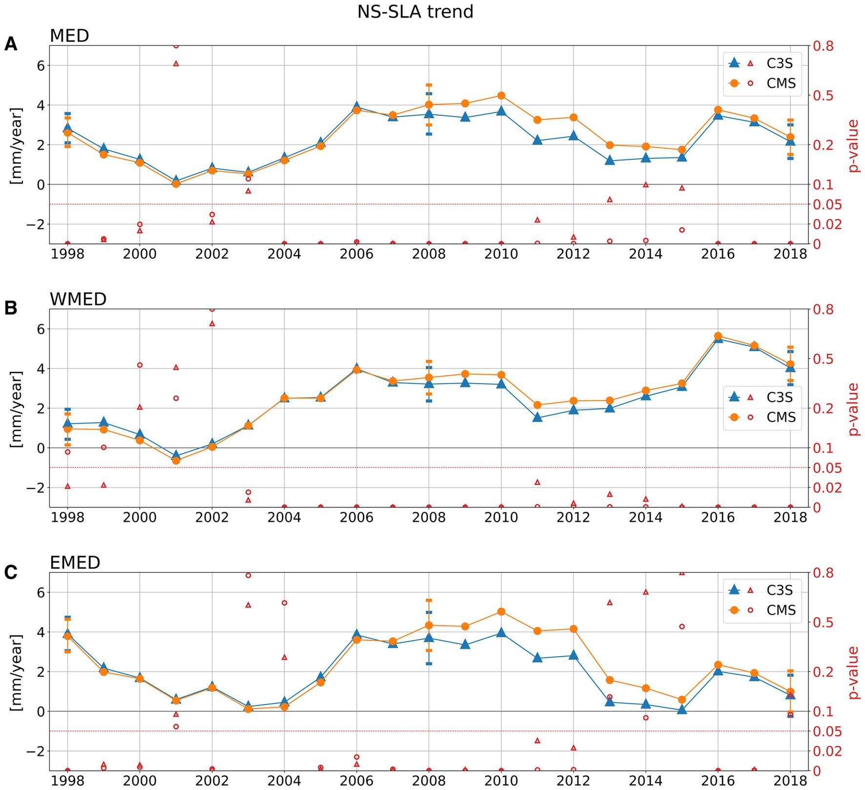
Figure 5. Timeseries of NS-SLA decadal trend values and correspondent statistical significance, computed over sliding windows shifted of 1 year over the period 1993–2022. The analysed regions are: MED (A), WMED (B), and EMED (C). CMS and C3S values are represented by circles and triangles, respectively. Continuous lines show the evolution of trend values across each decadal window, while red markers indicate the correspondent statistical significance. The threshold p-value of 0.05 is shown as a dashed red line, corresponding to a confidence interval of 95%. Error bars represent the trend uncertainty, based on the bootstrap procedure, computed for the decades reported in Table 1 (1993–2002, 2003–2012, and 2013–2022).

Aligned with SLA trends, Figure 6 presents tide gauge data from the Hadera, Venice, and Trieste stations, situated in the Levantine and Adriatic Seas, respectively. Notably, the tide gauges in the Adriatic Sea display a trend that turns negative in the last decade, consistent with the trend values depicted in Figure 3, while Hadera station shows only a deceleration.

Figure 6

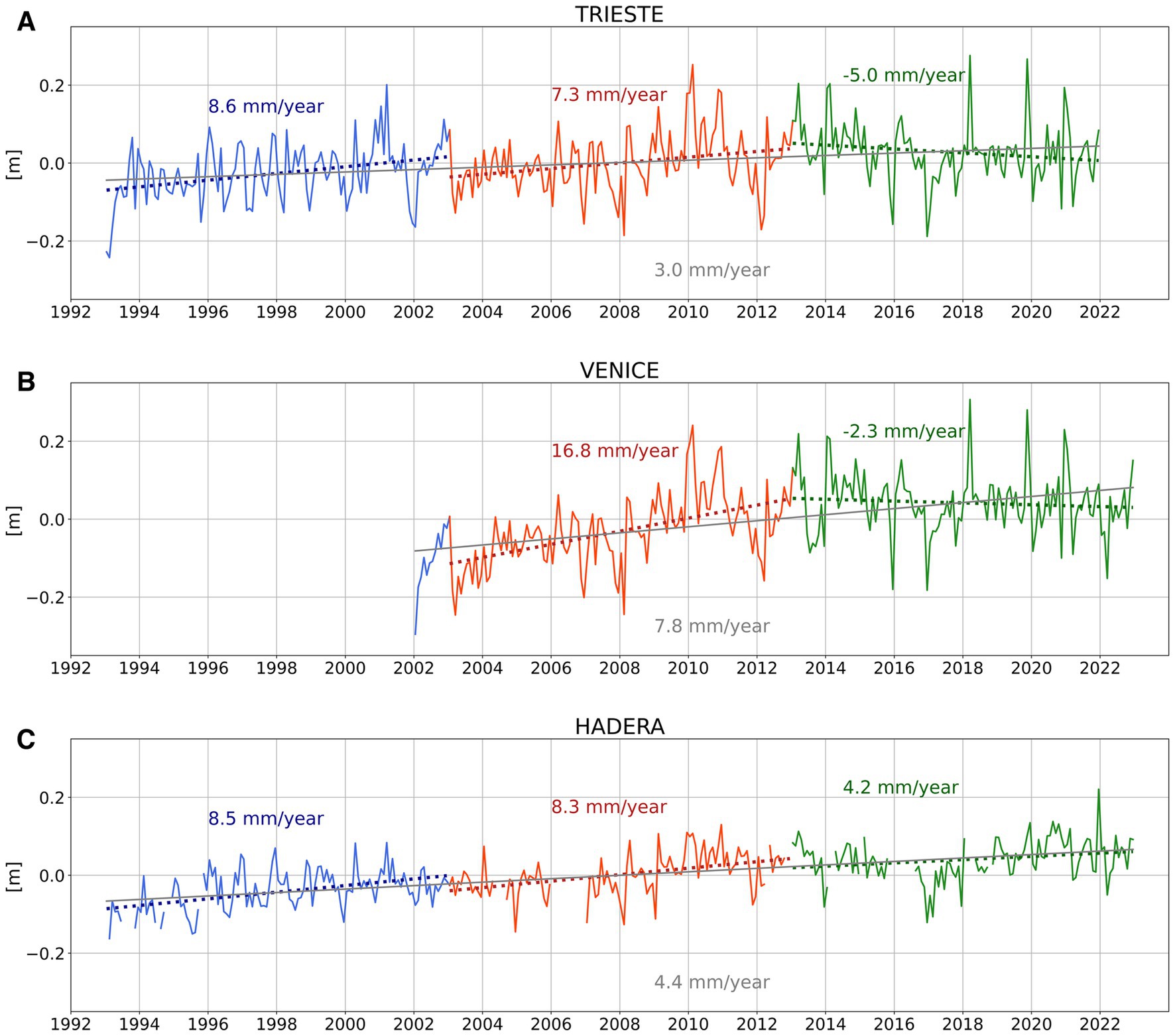
Figure 6. Timeseries of de-seasoned monthly mean sea level in Trieste (A), Venice (B), and Hadera (C) tide gauges from PSMSL dataset. Each decade has a different colour, and the linear fits are shown as dotted lines: 1993–2002 (blue), 2003–2012 (orange) and 2013–2022 (green). The thin black line represents the linear fit over the entire period. Trend values are superimposed to each fit. Trends in Trieste and Venice and reported in Table 2.

3.1.1 Adriatic Sea slowdown

Figure 7 depicts the geographical distribution of NS-SLA decadal trends observed in the Adriatic Sea using CMS and C3S datasets. In this region, the first two decades are characterised by a positive trend, with maximum values in the northern areas decreasing southward. The observed range is slightly lower in the second decade (Figures 7C,D) compared to the first (Figures 7A,B), but the most significant differences appear in the last decade (Figures 7E,F). Indeed, between 2013 and 2022, the NS-SLA trend reverse sign in most of the basin. This inversion is more pronounced around 44°N and 45°N, while weakly positive trends are still observed offshore southward of 43°N, particularly near the Otranto Strait. The observed trend in the last decade is statistically significant throughout the region, except in areas where it changes sign. As expected, the trend computed over the entire 30-year period masks the observed decadal sea level variations (Figures 7G,H), showing a positive value that is almost homogeneous over the entire region. In contrast, the variations between the decades differ according to the geographical location, with the highest negative trends observed in the northern Adriatic Sea.

Figure 7

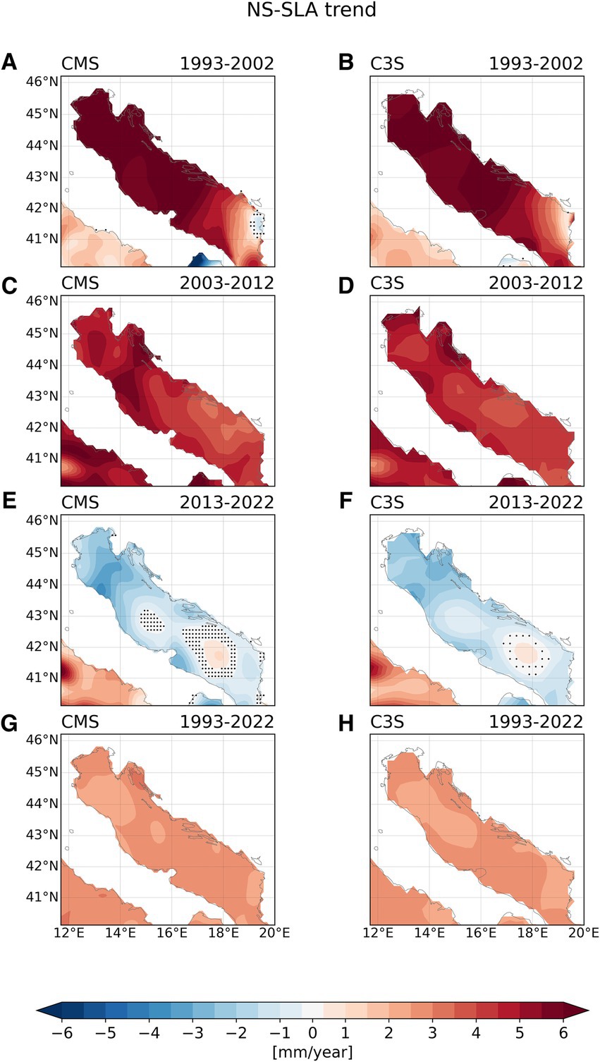
Figure 7. Zoom from Figure 3 in the Adriatic Sea: maps of NS-SLA trend from CMS (left) and C3S (right) datasets. The periods of estimated trend are: 1993–2002 (A,B), 2003–2012 (C,D), 2013–2022 (E,F), and 1993–2022 (G,H). The black dots indicate points where the p-values are larger than 0.05, so the trend estimation has no statistical significance.

The Adriatic slowdown during the last period is confirmed by analysing the decadal trend calculated using sliding time windows (Figure 8). Like the EMED, the trend is large during the initial period, then becomes negligible in the decades centered around 2004, peaks in the middle (around 6 mm/year), and declines to negligible values in the most recent time windows. The latest period (2013–2022) confirms a decrease in MSL trend at the subregional scale.

Figure 8

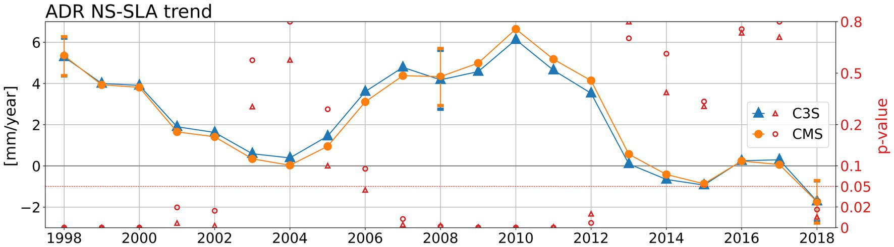
Figure 8. Timeseries of NS-SLA decadal trend values and correspondent statistical significance, computed over sliding windows shifted of 1 year over the period 1993–2022 in the Adriatic Sea. CMS and C3S values are represented by circles and triangles, respectively. Continuous lines show the evolution of trend values across each decadal window, while red markers indicate the correspondent statistical significance. The threshold p-value of 0.05 is shown as a dashed red line, corresponding to a confidence interval of 95%. Error bars represent the trend uncertainty, based on the bootstrap procedure, computed for the decades reported in Table 2 (1993–2002, 2003–2012, 2013–2022).

The Adriatic Sea trends for the three non-overlapped decades are summarised in Table 2. The trend value changes from the first to the second decade, decreasing from 5.3 ± 0.9 mm/year to 4.3 ± 1.4 mm/year for CMS (from 5.3 ± 0.9 to 4.2 ± 1.4 mm/year in C3S). The most significant change occurs during the third decade, where the sign reverses to reach −1.7 ± 1.0 mm/year both in CMS and C3S. The computed 30-year trend of 2.6 ± 0.3 mm/year is in agreement with the value reported by Meli et al. (2023) for the period 1993–2019, but here we describe the decadal local trends.

Table 2

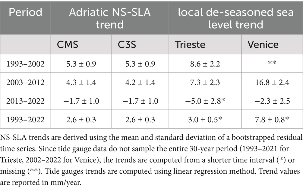
Table 2. Decadal and multidecadal trends of sea level in the Adriatic Sea, computed from daily time series of low-pass filtered NS-SLA from the CMS and C3S datasets, and time series of de-seasoned monthly mean sea level from PSMSL tide gauges.

The slowdown results in the Adriatic Sea are confirmed by the long-time records of tide gauges data in Trieste and Venice from the PSMSL dataset. Figure 6 and Table 2 report the timeseries and decadal trends computed from de-seasoned data.

In the case of Trieste, the timeseries at Molo Sartorio, previously analysed by Raicich (2023), reports a linear trend correspondent to 3.0 ± 0.5 mm/year over the 1993–2021 period. However, if we compute the decadal trend we find again the trend inversion: from 8.6 ± 2.2 mm/year (1993–2002) to 7.3 ± 2.3 mm/year (2003–2012), and then drastically decreasing to −5.0 ± 2.8 mm/year between 2013 and 2021. Therefore, the city of Trieste has recently experienced a sea level fall.

A similar phenomenon is reported at Faro San Nicolò just outside the Venice lagoon, although a shorter timeseries is available only from 2002 to 2022. In this case, the de-seasoned monthly mean sea level trend changes from 16.8 ± 2.4 mm/year (2003–2012) to a negative value of −2.3 ± 2.5 mm/year (2013–2022).

It is important to note that the PSMSL data have been adjusted to account for regional land subsidence. Nevertheless, the observed land subsidence rate of approximately −3 mm/year in Venice, as reported by Tosi et al. (2007), is less significant compared to the sea level trend variation calculated in this study.

3.1.2 Thermosteric and halosteric effects on the Mediterranean Sea MSL

This section describes the impact of water density changes induced by salinity and temperature variations on the MSL variability.

At the global scale, water thermal expansion is a significant factor contributing to GMSL (Llovel et al., 2023). In contrast, the salinity effects on sea level are poorly documented due to the scarcity of measurements (Wang et al., 2017). In the MED, in-situ observations confirm the positive temperature trend (Kubin et al., 2023) while the increased salinization has been explored both at the basin scale (Aydogdu et al., 2023) and at the regional scale (Potiris et al., 2024). The positive Adriatic Sea salinity trends were analysed in detail by Amorim et al. (2024) and Mihanović et al. (2021).

In this analysis, the thermosteric and halosteric terms are computed from MEDREA24 using a linear approximation of the equation of state EOS80 (Jackett and Mcdougall, 1995),

$\begin{array}{ll}{\eta }_s=-\underset{-H}{\overset{0}{{\displaystyle \int }}}\frac{{\rho }^{\prime }}{{\rho }_0}dz& (1)\end{array}$

$\begin{array}{ll}\frac{{\rho }^{\prime }}{{\rho }_0}=-\alpha \left(T-T_f\right)+\beta \left(S-S_f\right)& (2)\end{array}$

where ${\rho }_0$ , ${\mathrm{T}}_f$ , ${\mathrm{S}}_f$ are reference values of density, temperature, and salinity computed over the entire MED (Table 3). The linear thermosteric and halosteric coefficients, $\alpha$ and $\beta$ , are defined as temporal averages over the basin and reported in Table 3.

Table 3

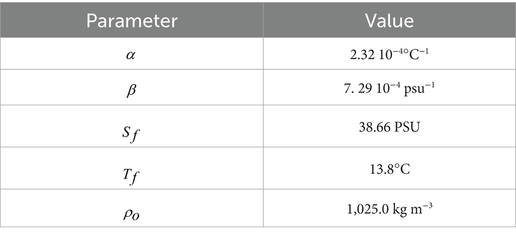
Table 3. Values of constant parameters in Equation 2.

Figure 9 shows the monthly timeseries of these components. In line with the GMSL, the thermosteric term increases the sea level by about 12 cm during the entire 1993–2022 period, with a seasonal cycle amplitude of about 9 cm. Conversely, the halosteric component decreases the sea level by a similar magnitude (~10 cm), with a negligible seasonal cycle. As a result, the halosteric and thermosteric components balance each other, reducing their impact on the MMSL rise. This finding agrees with the results of Calafat et al. (2012) that shows a small contribution from the steric sea level to the MMSL trend. It also agrees with Meli et al. (2023) who found that halosteric and thermosteric effects balance leaving a small steric sea level trend.

Figure 9

Figure 9. Timeseries of thermosteric, halosteric and total steric sea level components in the MED computed from MEDREA24 dataset using Equations 1 and 2 monthly values. Dashed vertical lines correspond to threshold years between decades, 2003 and 2013. Note the seasonal cycle that characterises the thermal and total steric monthly timeseries.

As for the sea level satellite datasets, Figure 10 illustrates the variability of the de-seasoned sea level steric component, with decadal trends computed over sliding windows for MED, WMED, EMED and Adriatic Sea. The steric trends oscillate around statistically non-significant values across all regions, consistent with the findings of the multidecadal analysis by Calafat et al. (2012). Apart from the WMED (Figure 10B), the third decade trends are either not significant or significantly negative, as in the cases of EMED (Figure 10C) and Adriatic (Figure 10D). We argue that the opposite sign trend between WMED and EMED in the last decade makes the overall MED trend (Figure 10A) statistically insignificant.

Figure 10

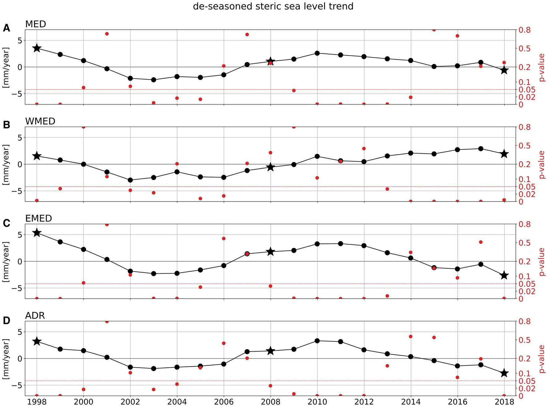
Figure 10. Timeseries of steric sea level decadal trend values from MEDREA24 and correspondent statistical significance, computed over sliding windows shifted of 1 year over the period 1993–2022. The analysed regions are: MED (A), WMED (B), EMED (C), and Adriatic Sea (D). For each decadal window, the black dot represents the trend value, while the red dot represents the trend statistical significance. The threshold p-value of 0.05 is shown as a dashed red line, corresponding to a confidence interval of 95%. Black stars in the MED and EMED correspond to trend values reported in Table 5.

3.2 The water budget contribution to the Mediterranean Sea MSL trend

In this section we investigate the contribution of the water budget to the MMSL and EM-MSL to demonstrate the reasons for the trend changes.

For any laterally open region of the world ocean, using an approximated continuity equation and averaging over the volume, the tendency in MSL is given by Pinardi et al. (2014).

$\begin{array}{ll}\frac{d\langle {\eta }_T\rangle }{dt}=\underset{1}{\underbrace{-\frac{{{\displaystyle \sum }}_i{T}_r^i}{\Omega }}}\underset{2}{\underbrace{-\langle q_w\rangle }}\underset{3}{\underbrace{+\frac{d\langle {\eta }_s\rangle }{dt}}}& (3)\end{array}$

where $\langle {\eta }_T\rangle$ is the MSL averaged over the area of the domain, called $\Omega$ , and $\eta s$ is defined in Equation 1. ${\displaystyle {\sum }_i{T}_i^r}$is the net volume transport in m³/s, positive outward from the lateral open boundaries. Additionally,

$\begin{array}{ll}{q}_w=E-P-R& (4)\end{array}$

is the surface water budget, considering the Evaporation (E), the Precipitation (P) and the river Runoff (R), the latter considered to be discharged at river points along the coasts. Term $3$ is the steric sea level trend that we evaluate from the analysis in section 3.1.2. The details of the derivation of Equation 3 are given in Pinardi et al. (2014) and more specifically in Masina et al. (2022). A comparable approach is proposed by Griffies and Greatbatch (2012) to identify the physical processes influencing the evolution of the mean sea level on a global scale.

The spatial extent, the complex coastline geometry, and the limited resolution of the available datasets do not provide sufficient accuracy to compute the MSL balance in the Adriatic region. However, this analysis is feasible in larger domains. Thus, we compute the terms in Equation 3 both for the entire MED and for the EMED.

Table 4 presents the decadal mean values for the components of Term 2 as given in Equation 4 and Term 1, while Table 5 show their sum with Term $3$ as described in Equation 3. It is important to note that Equation 3 represents a balance between large values, whose difference is of the same order of magnitude as the associated errors. Using independent datasets to estimate Terms 1 and 2 makes it challenging to derive a MSL tendency comparable with observations. Despite these limitations, the 30-year tendency obtained for the MMSL is of the right order of magnitude with respect to trend estimates from satellite data (Tables 1, 5).

Table 4

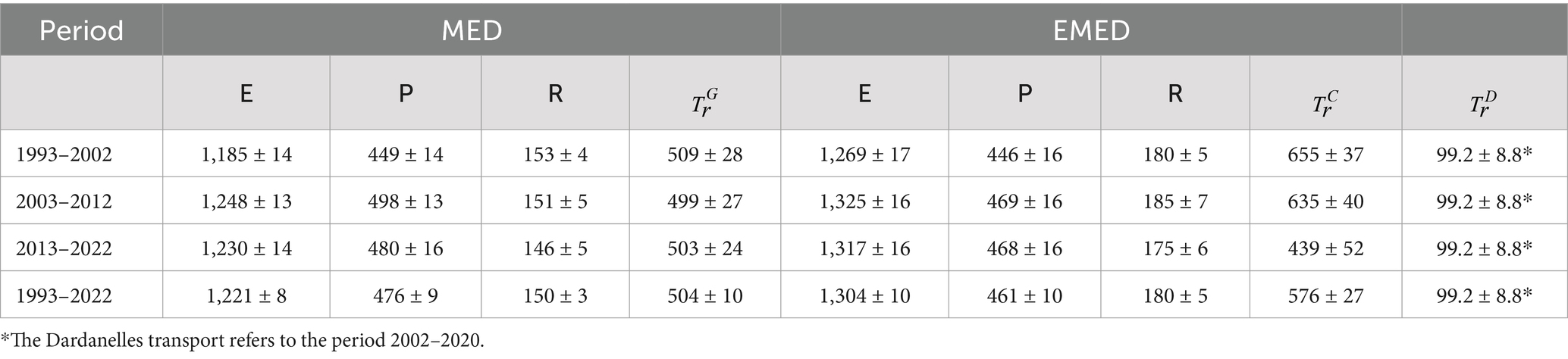
Table 4. Decadal and multidecadal mean values of different factors contributing to the MSL balance in the MED and EMED: evaporation and precipitation (E and P, from ERA5), river runoff (R, from EFASv5), and net zonal transport at the Gibraltar Strait ($T_r^G$, from MEDREA24), the Calabrian section ($T_r^C$, from MEDREA24) and the Dardanelles Strait ($T_r^D$, from Garcia-Garcia et al., 2022).

Table 5

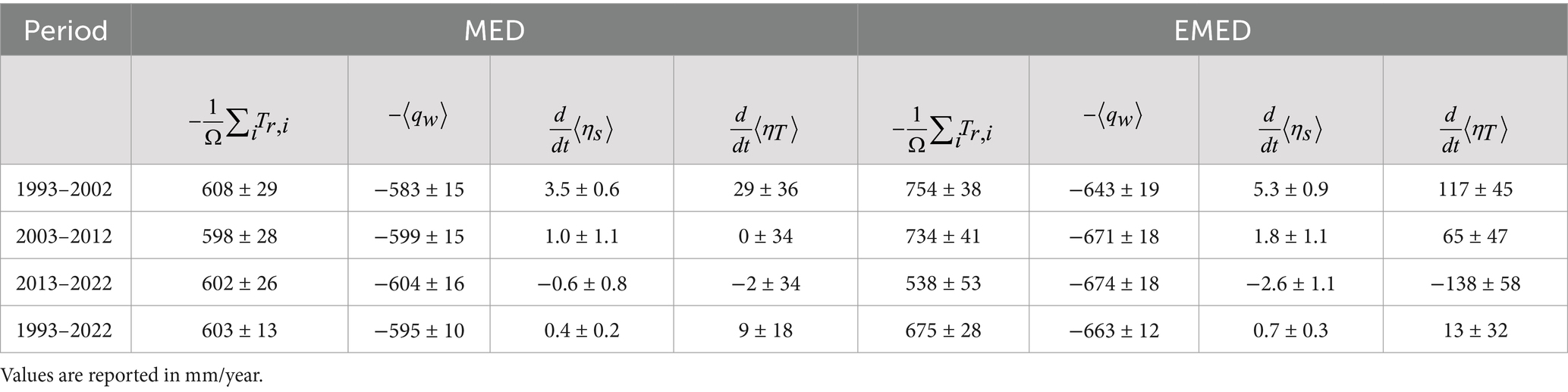
Table 5. Decadal and multidecadal mean values of Terms 1, 2 and 3 in Equation 3, and best estimate of the mean sea level terms balance in the MED and EMED.

Focusing on the steric decadal tendencies presented in Table 5, we find a slowdown during the three decades both in the MED and EMED. The trend reduction is more pronounced in the EMED, where values drop from 5.3 ± 0.9 mm/year to −2.6 ± 1.1 mm/year. The steric trend values are one order of magnitude smaller compared to the uncertainties associated to Terms 1 and 2, thus we conclude that the steric tendency term is a negligible contribution to the estimate of Equation 3.

We now analyse Term 1, representing the net volume transport across the open boundaries of the MED and EMED regions. The regions have in common the Dardanelles Strait ( $T_r^D$ ), while for the MED the other transport contribution comes from the Gibraltar Strait ( $T_r^G$ ), and for the EMED comes from the Calabrian section ( $T_r^C$ ). For the Dardanelles transport, we refer to García-García et al. (2022), assuming it is constant over the whole analysed period, since we are not aware of other data for the three decades. The time-mean net transport at Gibraltar is positive as well as the net volume transport at the Calabrian section (a comparison of the Gibraltar and Calabrian net transport from different reanalysis datasets is proposed in the Supplementary material).

Both the Gibraltar Strait and the Calabrian section net water transports are decreasing across the 1993–2022 period. However, while the decrease in Gibraltar is within the estimation errors, the change in the Calabrian section over the last decade represents 24% of the three-decade average transport. We believe the Calabrian transport value should be used with caution since the section at 16°E is an open ocean area section, not a Strait. Here circulation structures cut across the boundary at different depths, the flow field is extremely variable across the section, and we do not have any observed data in this region to validate the transport.

The Gibraltar net transport changes are connected to changes in inflow that are also correlated to different structures of the North Atlantic circulation, as documented by Masina et al. (2022). In their work they show that the inflow transport at Gibraltar is correlated with the MMSL as expected from Equation 3 since we can write:

$\begin{array}{ll}{T}_r^G=-T_{inflow}^G+T_{outflow}^G& (5)\end{array}$

where $T_{inflow}^G$ and $T_{outflow}^G$ are the Gibraltar inflow and outflow, respectively. Using Equation 5 in Equation 3 we expect positive changes in Gibraltar inflow to be associated with positive MMSL tendencies. Furthermore, Masina et al. (2022) reports that in the period 1993–2019, during years of weaker/stronger Atlantic Meridional Circulation, the Gibraltar inflow is stronger/weaker this giving rise to decadal variability.

We then analyze Term 2 for the MMSL and EM-MSL balances in Tables 4, 5. Changes in the surface water budget are comparable for the two regions. Both E and P increase from the 1993–2002 to 2003–2012 periods, but the increase in E is more significant than that of P when considering the associated errors. Moving into the third period, E and P values slightly decrease but remain higher than those observed in the 1993–2002 period. Variations in R are smaller between the first and second decade compared to the changes from the second to the third. Despite the uncertainties associated with each term, the increase in E is not offset by corresponding changes in P or R, leading to an overall decadal decrease of Term 2 in the sea level tendency equation 3.

The decadal slowdown of EM-MSL from C3S in Table 1 during the second period aligns more closely with the increased absolute value of the surface water budget (Term 2) than with the CMS trend, which continues to grow in the second decade despite significant changes in the EMED water budget. As previously discussed, this discrepancy may be attributed to the differing sampling frequencies of the input satellite observation systems rather than reflecting a genuine signal, as evidenced by the C3S dataset.

Based on this, we propose an interpretation of the MSL slowdown: the observed changes in the water budget, driven primarily by increased E, have reduced the sea level trend across the entire MED. In the EMED the decreasing sea level tendency is greater due to a concomitant decreasing transport across the Calabrian section which is connected to changes in circulation patterns.

Both the MMSL and EM-MSL tendencies support the hypothesis that the observed slowdown is driven by changes in the basins’ water budgets, specifically Terms 1 and 2. However, the tendencies in the EMED are larger than anticipated, with a notably significant negative EM-MSL tendency (as shown in Table 5) and higher associated errors compared to the MMSL tendency.

We propose several reasons for this discrepancy:

1. The ERA5 and EFAS datasets, used to estimate Term 2, are not utilized in the reanalysis, leading to imbalances with Gibraltar transport. The MEDREA24 water budget differs from that of ERA5 and EFAS because MEDREA24 calculates evaporation based on ERA5 winds, air temperature, and dew point while still employing an outdated runoff formulation (Escudier et al., 2021).

2. The Dardanelles net outflow is assumed to be constant over three decades due to a lack of data. This assumption likely has a greater impact on the EM-MSL than on the MMSL tendency. Additionally, in MEDREA24, the Dardanelles Strait is represented as an inverse river (Escudier et al., 2021), which complicates its relationship to net transport.

Despite these limitations, we argue that the EMED slowdown must result from changes in the regional water budget consisting of Term 1 and 2. Equation 3, which governs the MSL tendency, supports this conclusion, as steric contributions are minimal.

4 Discussion

Our findings emphasize the critical role of the Mediterranean’s water budget in shaping sea level trends and highlight the regional complexity of decadal changes. Continued monitoring and deeper insights into regional water balance dynamics are essential for improving climate projections and informing climate adaptation strategies for Mediterranean coastal regions.

It is well known that the Global MSL rise is due to the increased positive tendency in both mass (Term 2 only) and steric components (Term 3′) (IPCC, 2023; Milne et al., 2009). Conversely, in the Mediterranean Sea, thermal expansion and haline contraction compensate each other over the last 30 years, resulting in a minimal total steric sea level tendency (Meli et al., 2023). Therefore, we argue that changes in the Mediterranean MSL are driven by the mass component terms of the MSL equation 3.

Examining the mass terms reveals that the most significant decadal differences arise from the imbalance between inward net transports and surface water fluxes, especially in the Eastern Mediterranean. In this region, the inward transport tendency weakened over successive decades, accompanied by an increase in evaporation that was not offset by precipitation and runoff. This analysis identifies increased evaporation and decreased runoff as the most significant drivers of the MSL decadal slowdown, particularly in the Eastern Mediterranean.

To compare the observed 30-year MMSL trend with other regions of European seas, we refer to the recent work of Melet et al. (2024) in the framework of the European Sea Level Rise Assessment Report (van den Hurk et al., 2024). In agreement with the results presented in this study, Figure 6 in Melet et al. (2024) show that the MSL trend in the Mediterranean is lower than the European average (~1.5 mm/year compared to 3.2 mm/year). The same figure highlights specific regions where the trend has an opposite behaviour, with values exceeding the European mean.

The knowledge of decadal and longer term sea level trends is at the basis of climate adaptation strategies as documented recently by Galluccio et al. (2024). In their review of the adaptation measures to sea level rise they point out to the possible responses to sea level changes: (i) accommodate, (ii) protect, (iii) advance and (iv) retreat. The Climate Change Adaption Digital Twin initiative in Europe is developing the strategy to make accessible multi-decadal streams of data for climate risk assessment. An initial study by Malakar et al. (2024) documents the positive impact that decadal projections have on agricultural farmer strategies instead of longer-term climate projections. Given the importance of these trends for actionable climate strategies, our study suggests the importance of decadal analysis of sea level trends in support of coastal adaptation plans. Furthermore, Srivastava et al. (2022) stresses that the adaptation measures have no stringent approach; instead, it is site-specific as well as context specific. We suggest here that decadal trend variability might be important for policy making at the level of the Adriatic Sea and the Eastern Mediterranean.

Building on this foundation, we compare our observational analysis with recent studies to identify consistent trends and validate findings. In particular, our observational analysis is consistent with the findings of a climate downscaling analysis in the Adriatic Sea by Verri et al. (2024, hereafter Verri2024) and the sea level trend analysis by da Costa et al. (2024). Verri2024 provides a projection under the RCP8.5 scenario through 2050, while da Costa et al. (2024) examines historical and projected changes. Both studies identify a multi-decadal slowdown in the northern Adriatic (see Figure 14 in Verri2024), attributed to the limited steric effect caused by salinization. The Verri2024 study highlights the uncertainties inherent in climate downscaling approaches, particularly in modeling the atmosphere-hydrology-oceanographic water cycle at high resolution nested within low-resolution regional projection data. Additionally, Verri2024 focuses on multi-decadal changes in projections without addressing interdecadal variability.

Given the uncertainties identified in these studies, our results emphasize the need, in the coming years, to advance climate downscaling by validating projections against observed sea level decadal changes derived from tide gauges and satellite altimetry. In this context, we provide reference results for the 1993–2022 period, which should be extended and continuously updated.

5 Conclusion

Sea level observations over the Mediterranean Sea have been analysed over decadal periods from 1993 to 2022, revealing an acceleration of the Mediterranean Mean Sea Level (MSL) trend from the first to the second decade, followed by a notable slowdown in the last decade.

Analysing altimeter satellite data, the Mediterranean Sea exhibits an overall MSL trend of 2.4 ± 0.2 mm/year according to C3S dataset (2.6 ± 0.2 mm/year in CMS dataset), with a nearly uniform value across the basin. However, when examining decadal trends, distinct behaviours are observed between the western and eastern parts of the domain. The western part shows an increasing positive trend in agreement with the global ocean estimates, while the eastern part tends towards negative values, resulting in a Mediterranean Sea overall slowdown. Specifically, the slowdown observed at the overall Mediterranean scale from the second to the third decade (from 3.6 ± 1.0 mm/year to 2.2 ± 0.8 mm/year according to C3S dataset) is primarily driven by the weak and negative Non-Seasonal Sea Level Anomaly (NS-SLA) trend in the eastern part of the domain, where the NS-SLA trend drops from 3.7 ± 1.3 mm/year to 0.8 ± 1.0 mm/year.

Significant variations are noted in the semi-enclosed Aegean and Adriatic Seas, where sea level rise was initially consistent with the basin mean (from 1993 to 2012) but then reversed, starting to drop in the last decade. Negative trends in the Adriatic Sea over the last 10 years have also been confirmed by tide gauge data, corroborating the satellite observations.

Our results indicate that the slowdown of the Mediterranean MSL and its eastern subdomain are due to the combined effects of changes in the water budget and the balance between thermal expansion and haline contraction. The decadal changes in the water deficit of the Mediterranean Sea show a consistent trend towards higher water losses by evaporation not compensated by precipitation, runoff and transport across Straits. These results bring definitive evidence to the conclusions of Calafat et al. (2012) for the importance of the water budget in the Mediterranean Sea level trend and Meli et al. (2023) for the steric compensation.

Despite all the limitations, the study analyses for the first time the MSL tendency equation for decadal periods. We emphasize the complexity of modelling and interpreting MSL tendencies, highlighting the importance of reconciling different datasets and reanalysis approaches. Understanding decadal and longer-term sea level trends, as documented by Galluccio et al. (2024), is fundamental for climate adaptation strategies, and this study advances their analysis by providing a foundation for more reliable projections and facilitating coastal adaptation plans.

In the future, we suggest a dedicated effort to monitor water transport across sections of the Mediterranean basin, as well as a continued focus on evaluating changes in the surface water budget. These factors are likely to play a critical role in driving MSL changes across the basin, leading to a more detailed assessment of significant hazards and impacts.

Data availability statement

Publicly available datasets analyzed in this study are referenced in the text. Other data and codes used to perform the analysis are available on the Zenodo Repository at: https://doi.org/10.5281/zenodo.14725778 (Borile et al., 2025).

Author contributions

FB: Writing – original draft, Writing – review & editing, Conceptualization, Formal analysis, Investigation, Visualization, Data curation, Methodology, Software. NP: Writing – original draft, Writing – review & editing, Conceptualization, Funding acquisition, Methodology, Investigation. VL: Data curation, Formal analysis, Software, Visualization, Investigation, Writing – review & editing. MG: Data curation, Formal analysis, Investigation, Software, Visualization, Writing – review & editing. ANa: Writing – review & editing, Investigation. JA: Investigation, Writing – review & editing. EC: Investigation, Writing – review & editing. GC: Investigation, Writing – review & editing. LM: Writing – review & editing, Investigation. GV: Investigation, Writing – review & editing. VS: Investigation, Writing – review & editing. ES: Data curation, Investigation, Writing – review & editing. FM: Data curation, Investigation, Writing – review & editing. ANo: Data curation, Investigation, Writing – review & editing. PO: Writing – review & editing, Conceptualization, Investigation, Methodology.

Funding

The author(s) declare that financial support was received for the research, authorship, and/or publication of this article. This work has received funding from the AdriaClim project, Italy (Climate change information, monitoring and management tools for adaptation strategies in Adriatic coastal areas; project ID 10252001). This study was also carried out within the RETURN Extended Partnership and received funding from the European Union Next-Generation EU (National Recovery and Resilience Plan – NRRP, Mission 4, Component 2, Investment 1.3 – D.D. 1243 2/8/2022, PE0000005).

Acknowledgments

The authors are thankful for the support offered by the CMCC Regional Ocean Forecasting System Division and especially Rita Lecci support in using them.

Conflict of interest

FM and ANo were employed by company ETT SpA.

The remaining authors declare that the research was conducted in the absence of any commercial or financial relationships that could be construed as a potential conflict of interest.

The author(s) declared that they were an editorial board member of Frontiers, at the time of submission. This had no impact on the peer review process and the final decision.

Publisher’s note

All claims expressed in this article are solely those of the authors and do not necessarily represent those of their affiliated organizations, or those of the publisher, the editors and the reviewers. Any product that may be evaluated in this article, or claim that may be made by its manufacturer, is not guaranteed or endorsed by the publisher.

Supplementary material

The Supplementary material for this article can be found online at: https://www.frontiersin.org/articles/10.3389/fclim.2025.1472731/full#supplementary-material

References

Ablain, M., Meyssignac, B., Zawadzki, L., Jugier, R., Ribes, A., Spada, G., et al. (2019). Uncertainty in satellite estimates of global mean sea-level changes, trend and acceleration. Earth Syst. Sci. Data 11, 1189–1202. doi: 10.5194/essd-11-1189-2019

Crossref Full Text | Google Scholar

Adani, M., Dobricic, S., and Pinardi, N. (2011). Quality assessment of a 1985–2007 Mediterranean Sea reanalysis.

Google Scholar

Adcroft, A., and Campin, J.-M. (2004). Rescaled height coordinates for accurate representation of free-surface flows in ocean circulation models. Ocean Model 7, 269–284. doi: 10.1016/j.ocemod.2003.09.003

Crossref Full Text | Google Scholar

Alessandri, J., Pinardi, N., Federico, I., and Valentini, A. (2023). Storm surge ensemble prediction system for lagoons and transitional environments.

Google Scholar

Amorim, F. L. L., Le Meur, J., Wirth, A., and Cardin, V. (2024). Tipping of the double-diffusive regime in the southern Adriatic pit in 2017 in connection with record high-salinity values. Ocean Sci. 20, 463–474. doi: 10.5194/os-20-463-2024

Crossref Full Text | Google Scholar

Aydogdu, A., Miraglio, P., Escudier, R., Clementi, E., and Masina, S. (2023). The dynamical role of upper layer salinity in the Mediterranean Sea. State Planet 1-osr7, 1–9. doi: 10.5194/sp-1-osr7-6-2023

Crossref Full Text | Google Scholar

Bonaduce, A., Pinardi, N., Oddo, P., Spada, G., and Larnicol, G. (2016). Sea-level variability in the Mediterranean Sea from altimetry and tide gauges. Clim. Dyn. 47, 2851–2866. doi: 10.1007/s00382-016-3001-2

PubMed Abstract | Crossref Full Text | Google Scholar

Calafat, F. M., Chambers, D. P., and Tsimplis, M. N. (2012). Mechanisms of decadal sea level variability in the eastern North Atlantic and the Mediterranean Sea. J. Geophys. Res. Oceans 117:8285. doi: 10.1029/2012JC008285

Crossref Full Text | Google Scholar

Cazenave, A., Dieng, H.-B., Meyssignac, B., von Schuckmann, K., Decharme, B., and Berthier, E. (2014). The rate of sea-level rise. Nat. Clim. Chang. 4, 358–361. doi: 10.1038/nclimate2159

Crossref Full Text | Google Scholar

Cessi, P., Pinardi, N., and Lyubartsev, V. (2014). Energetics of Semienclosed Basins with Two-Layer Flows at the Strait.

Google Scholar

Chelton, D. B., and Schlax, M. G. (2003). The accuracies of Smoothed Sea surface height fields constructed from tandem satellite altimeter datasets. Available at: https://journals.ametsoc.org/view/journals/atot/20/9/1520-0426_2003_020_1276_taosss_2_0_co_2.xml

Google Scholar

Criado-Aldeanueva, F., Del Río Vera, J., and García-Lafuente, J. (2008). Steric and mass-induced Mediterranean Sea level trends from 14 years of altimetry data. Glob. Planet. Chang. 60, 563–575. doi: 10.1016/j.gloplacha.2007.07.003

PubMed Abstract | Crossref Full Text | Google Scholar

Dangendorf, S., Hay, C., Calafat, F. M., Marcos, M., Piecuch, C. G., Berk, K., et al. (2019). Persistent acceleration in global sea-level rise since the 1960s. Nat. Clim. Chang. 9, 705–710. doi: 10.1038/s41558-019-0531-8

Crossref Full Text | Google Scholar

da Costa, V. S., Alessandri, J., Verri, G., Mentaschi, L., Guerra, R., and Pinardi, N. (2024). Marine climate indicators in the Adriatic Sea. Front. Clim. 6:1449633. doi: 10.3389/fclim.2024.1449633

PubMed Abstract | Crossref Full Text | Google Scholar

Dobricic, S., and Pinardi, N. (2008). An oceanographic three-dimensional variational data assimilation scheme. Ocean Model 22, 89–105. doi: 10.1016/j.ocemod.2008.01.004

PubMed Abstract | Crossref Full Text | Google Scholar

Escudier, R., Clementi, E., Cipollone, A., Pistoia, J., Drudi, M., Grandi, A., et al. (2021). A high resolution reanalysis for the Mediterranean Sea. Front. Earth Sci. 9:702285. doi: 10.3389/feart.2021.702285

Crossref Full Text | Google Scholar

European Seas Gridded L 4 Sea Surface Heights and Derived Variables Reprocessed 1993 Ongoing (n.d.). E. U. Copernicus Marine Service Information (CMEMS). Marine Data Store (MDS). doi: 10.48670/moi-00141 (Accessed June 16, 2024).

Crossref Full Text | Google Scholar

Galluccio, G., Hinkel, J., Fiorini Beckhauser, E., Bisaro, A., Biancardi Aleu, R., Campostrini, P., et al. (2024). Sea level rise in Europe: adaptation measures and decision-making principles. State Planet 3-slre1, 1–31. doi: 10.5194/sp-3-slre1-6-2024

Crossref Full Text | Google Scholar

García-García, D., Vigo, M. I., Trottini, M., Vargas-Alemañy, J. A., and Sayol, J.-M. (2022). Hydrological cycle of the Mediterranean-Black Sea system. Clim. Dyn. 59, 1919–1938. doi: 10.1007/s00382-022-06188-2

PubMed Abstract | Crossref Full Text | Google Scholar

Global Ocean Gridded L4 Sea Surface Heights and Derived Variables Reprocessed Copernicus Climate Service (n.d.). E. U. Copernicus Marine Service Information (CMEMS). Marine Data Store (MDS). doi: 10.48670/moi-00145 (Accessed June 16, 2024).

Crossref Full Text | Google Scholar

Griffies, S. M., and Greatbatch, R. J. (2012). Physical processes that impact the evolution of global mean sea level in ocean climate models. Ocean Model 51, 37–72. doi: 10.1016/j.ocemod.2012.04.003

Crossref Full Text | Google Scholar

Guérou, A., Meyssignac, B., Prandi, P., Ablain, M., Ribes, A., and Bignalet-Cazalet, F. (2023). Current observed global mean sea level rise and acceleration estimated from satellite altimetry and the associated measurement uncertainty. Ocean Sci. 19, 431–451. doi: 10.5194/os-19-431-2023

Crossref Full Text | Google Scholar

Hamed, K. H., and Ramachandra Rao, A. (1998). A modified Mann-Kendall trend test for autocorrelated data. J. Hydrol. 204, 182–196. doi: 10.1016/S0022-1694(97)00125-X

PubMed Abstract | Crossref Full Text | Google Scholar

Hay, C. C., Morrow, E., Kopp, R. E., and Mitrovica, J. X. (2015). Probabilistic reanalysis of twentieth-century sea-level rise. Nature 517, 481–484. doi: 10.1038/nature14093

PubMed Abstract | Crossref Full Text | Google Scholar

Hersbach, H., Bell, B., Berrisford, P., Hirahara, S., Horányi, A., Muñoz-Sabater, J., et al. (2020). The ERA5 global reanalysis. Q. J. R. Meteorol. Soc. 146, 1999–2049. doi: 10.1002/qj.3803

Crossref Full Text | Google Scholar

Holgate, S. J., Matthews, A., Woodworth, P. L., Rickards, L. J., Tamisiea, M. E., Bradshaw, E., et al. (2012). New data systems and products at the permanent service for mean sea level. J. Coast. Res. 29, 493–504. doi: 10.2112/JCOASTRES-D-12-00175.1

PubMed Abstract | Crossref Full Text | Google Scholar

Ioannou, A., Stegner, A., Le Vu, B., Taupier-Letage, I., and Speich, S. (2017). Dynamical evolution of intense Ierapetra eddies on a 22 year long period. J. Geophys. Res. Oceans 122, 9276–9298. doi: 10.1002/2017JC013158

Crossref Full Text | Google Scholar

IPCC (2023) in Climate change 2023: Synthesis report. Contribution of working groups I, II and III to the sixth assessment report of the intergovernmental panel on climate change. eds. Core Writing Team , H. Lee and J. Romero (Geneva, Switzerland: IPCC), 35–115.

Google Scholar

Jackett, D. R., and Mcdougall, T. J. (1995). Minimal adjustment of hydrographic profiles to achieve static stability. Available at: https://journals.ametsoc.org/view/journals/atot/12/2/1520-0426_1995_012_0381_maohpt_2_0_co_2.xml

Google Scholar

Jordà, G., Sánchez-Román, A., and Gomis, D. (2017). Reconstruction of transports through the strait of Gibraltar from limited observations. Clim. Dyn. 48, 851–865. doi: 10.1007/s00382-016-3113-8

PubMed Abstract | Crossref Full Text | Google Scholar

Kendall, M. G. (1948). Rank correlation methods : Griffin.

Google Scholar

Kubin, E., Menna, M., Mauri, E., Notarstefano, G., Mieruch, S., and Poulain, P.-M. (2023). Heat content and temperature trends in the Mediterranean Sea as derived from Argo float data. Front. Mar. Sci. 10:1271638. doi: 10.3389/fmars.2023.1271638

Crossref Full Text | Google Scholar

Llovel, W., Balem, K., Tajouri, S., and Hochet, A. (2023). Cause of substantial global mean sea level rise over 2014–2016. Geophys. Res. Lett. 50:e2023GL104709. doi: 10.1029/2023GL104709

Crossref Full Text | Google Scholar

Madec, G., Bourdallé-Badie, R., Bouttier, P.-A., Bricaud, C., Bruciaferri, D., Calvert, D., et al. (2017). NEMO Ocean engine [report].

Google Scholar

Malakar, Y., Snow, S., Fleming, A., Fielke, S., Jakku, E., Tozer, C., et al. (2024). Multi-decadal climate services help farmers assess and manage future risks. Nat. Clim. Chang. 14, 586–591. doi: 10.1038/s41558-024-02021-2

Crossref Full Text | Google Scholar

Mann, H. B. (1945). Nonparametric tests against trend. Econometrica 13, 245–259. doi: 10.2307/1907187

Crossref Full Text | Google Scholar

Masina, S., Pinardi, N., Banerjee, D. S., Lyubartsev, V., von Schuckmann, K., Jackson, L., et al. (2022). The Atlantic MeridionalOverturning circulation forcing the mean sealevel in the Mediterranean Sea through theGibraltar transport, Copernicus Ocean state report, issue 6. J. Oper. Oceanogr. 15, 1–220. doi: 10.1080/1755876X.2022.2095169

PubMed Abstract | Crossref Full Text | Google Scholar

Mediterranean Sea Mean Sea Level time series and trend from Observations Reprocessing (n.d.). E. U. Copernicus marine service information (CMEMS). Marine data store (MDS).doi: 10.48670/moi-00264 (Accessed July 24, 2024).

Crossref Full Text | Google Scholar

Melet, A., van de Wal, R., Amores, A., Arns, A., Chaigneau, A. A., Dinu, I., et al. (2024). Sea level rise in Europe: observations and projections. State Planet 3-slre1, 1–60. doi: 10.5194/sp-3-slre1-4-2024

Crossref Full Text | Google Scholar

Meli, M. (2024). The potential recording of north Ionian Gyre’s reversals as a decadal signal in sea level during the instrumental period. Sci. Rep. 14:4907. doi: 10.1038/s41598-024-55579-4

PubMed Abstract | Crossref Full Text | Google Scholar

Meli, M., Camargo, C. M. L., Olivieri, M., Slangen, A. B. A., and Romagnoli, C. (2023). Sea-level trend variability in the Mediterranean during the 1993–2019 period. Front. Mar. Sci. 10:1150488. doi: 10.3389/fmars.2023.1150488

Crossref Full Text | Google Scholar

Merrifield, M. A., Merrifield, S. T., and Mitchum, G. T. (2009). An anomalous recent acceleration of global sea level rise.

Google Scholar

Mihanović, H., Vilibić, I., Šepić, J., Matić, F., Ljubešić, Z., Mauri, E., et al. (2021). Observation, preconditioning and recurrence of exceptionally high salinities in the Adriatic Sea. Front. Mar. Sci. 8:672210. doi: 10.3389/fmars.2021.672210

Crossref Full Text | Google Scholar

Milne, G. A., Gehrels, W. R., Hughes, C. W., and Tamisiea, M. E. (2009). Identifying the causes of sea-level change. Nat. Geosci. 2, 471–478. doi: 10.1038/ngeo544

Crossref Full Text | Google Scholar

Mohamed, B., Abdallah, A. M., Alam El-Din, K., Nagy, H., and Shaltout, M. (2019). Inter-annual variability and trends of sea level and sea surface temperature in the Mediterranean Sea over the last 25 years. Pure Appl. Geophys. 176, 3787–3810. doi: 10.1007/s00024-019-02156-w

Crossref Full Text | Google Scholar

Montgomery, D. C., and Runger, G. C. (2018). Applied statistics and probability for engineers. 7th Edn. Hoboken NJ: Wiley.

Google Scholar

Moreira, L., Cazenave, A., and Palanisamy, H. (2021). Influence of interannual variability in estimating the rate and acceleration of present-day global mean sea level. Glob. Planet. Chang. 199:103450. doi: 10.1016/j.gloplacha.2021.103450

Crossref Full Text | Google Scholar

Patton, A., Politis, D. N., and White, H. (2009). Correction to “a utomatic block-length selection for the dependent bootstrap” by D. Politis and H. White. Econ. Rev. doi: 10.1080/07474930802459016

Crossref Full Text | Google Scholar

Pinardi, N., Bonaduce, A., Navarra, A., Dobricic, S., and Oddo, P. (2014). The mean sea level equation and its application to the Mediterranean Sea.

Google Scholar

Pinardi, N., Cessi, P., Borile, F., and Wolfe, C. L. P. (2019). The Mediterranean Sea overturning circulation. J. Phys. Oceanogr. 49, 1699–1721. doi: 10.1175/JPO-D-18-0254.1

Crossref Full Text | Google Scholar

Pinardi, N., Zavatarelli, M., Adani, M., Coppini, G., Fratianni, C., Oddo, P., et al. (2015). Mediterranean Sea large-scale low-frequency ocean variability and water mass formation rates from 1987 to 2007: a retrospective analysis. Prog. Oceanogr. 132, 318–332. doi: 10.1016/j.pocean.2013.11.003

Crossref Full Text | Google Scholar

Politis, D. N., and Romano, J. P. (1994). The stationary bootstrap. J. Am. Stat. Assoc. 89, 1303–1313. doi: 10.1080/01621459.1994.10476870

Crossref Full Text | Google Scholar

Potiris, M., Mamoutos, I. G., Tragou, E., Zervakis, V., Kassis, D., and Ballas, D. (2024). Dense water formation variability in the Aegean Sea from 1947 to 2023. Oceans 5, 611–636. doi: 10.3390/oceans5030035

PubMed Abstract | Crossref Full Text | Google Scholar

Raicich, F. (2023). The sea level time series of Trieste, Molo Sartorio, Italy (1869–2021). Earth Syst. Sci. Data 15, 1749–1763. doi: 10.5194/essd-15-1749-2023

Crossref Full Text | Google Scholar

Sen, P. K. (1968). Estimates of the regression coefficient based on Kendall’s tau. J. Am. Stat. Assoc. 63, 1379–1389. doi: 10.1080/01621459.1968.10480934

Crossref Full Text | Google Scholar

Smith, P. J., Pappenberger, F., Wetterhall, F., Thielen del Pozo, J., Krzeminski, B., Salamon, P., et al. (2016). “Chapter 11—on the operational implementation of the European flood awareness system (EFAS)” in Flood forecasting. eds. T. E. Adams and T. C. Pagano (Academic Press), 313–348.

Google Scholar

Srivastava, A., Maity, R., and Desai, V. R. (2022). “Assessing global-scale synergy between adaptation, mitigation, and sustainable development for projected climate change” in Ecological footprints of climate change: adaptive approaches and sustainability. eds. U. Chatterjee, A. O. Akanwa, S. Kumar, S. K. Singh, and A. Dutta Roy (Springer International Publishing), 31–61.

Google Scholar

Stammer, D., Cazenave, A., Ponte, R. M., and Tamisiea, M. E. (2013). Causes for contemporary regional Sea level changes. Annu. Rev. Mar. Sci. 5, 21–46. doi: 10.1146/annurev-marine-121211-172406

PubMed Abstract | Crossref Full Text | Google Scholar

Stocchi, P., and Davolio, S. (2017). Intense air-sea exchanges and heavy orographic precipitation over Italy: the role of Adriatic Sea surface temperature uncertainty. Atmos. Res. 196, 62–82. doi: 10.1016/j.atmosres.2017.06.004

Crossref Full Text | Google Scholar

Theil, H. (1992). “A rank-invariant method of linear and polynomial regression analysis” in Henri Theil’s contributions to economics and econometrics: Econometric theory and methodology. eds. B. Raj and J. Koerts (Netherlands: Springer), 345–381.

Google Scholar

Tosi, L., Teatini, P., Carbognin, L., and Frankenfield, J. (2007). A new project to monitor land subsidence in the northern Venice coastland (Italy). Environ. Geol. 52, 889–898. doi: 10.1007/s00254-006-0530-8

Crossref Full Text | Google Scholar

van den Hurk, B., Pinardi, N., Bisaro, A., Galluccio, G., Jiménez, J. A., Larkin, K., et al. (2024). Sea level rise in Europe: summary for policymakers. State Planet 3-slre1, 1–10. doi: 10.5194/sp-3-slre1-1-2024

Crossref Full Text | Google Scholar

Verri, G., Furnari, L., Gunduz, M., Senatore, A., Santos da Costa, V., De Lorenzis, A., et al. (2024). Climate projections of the Adriatic Sea: role of river release. Front. Clim. 6:1368413. doi: 10.3389/fclim.2024.1368413

Crossref Full Text | Google Scholar

Vigo, I., Garcia, D., and Chao, B. (2005). Change of sea level trend in the Mediterranean and black seas. J. Mar. Res. 63, 1085–1100. doi: 10.1357/002224005775247607

Crossref Full Text | Google Scholar

Wang, G., Cheng, L., Boyer, T., and Li, C. (2017). Halosteric Sea level changes during the Argo era. Water 9:484. doi: 10.3390/w9070484

PubMed Abstract | Crossref Full Text | Google Scholar

Watson, C. S., White, N. J., Church, J. A., King, M. A., Burgette, R. J., and Legresy, B. (2015). Unabated global mean sea-level rise over the satellite altimeter era. Nat. Clim. Chang. 5, 565–568. doi: 10.1038/nclimate2635

Crossref Full Text | Google Scholar

WCRP Global Sea Level Budget Group (2018). Global sea-level budget 1993–present. Earth Syst. Sci. Data 10, 1551–1590. doi: 10.5194/essd-10-1551-2018

Crossref Full Text | Google Scholar

Welch, B. L. (1947). The generalization of ‘student’s’ problem when several different population variances are involved. Biometrika 34, 28–35. doi: 10.2307/2332510

PubMed Abstract | Crossref Full Text | Google Scholar

World Meteorological Organization (2024). State of the global climate 2023. Geneva: WMO.

Google Scholar