A scientometrics review of conventional and soft computing methods in the slope stability analysis

Predicting slope stability is important for preventing and mitigating landslide disasters. This paper examines the existing approaches for analyzing slope stability. There are several established conventional approaches for slope stability analysis that can be applied in this context. However, in recent decades, soft computing methods has been extensively developed and employed in stochastic slope stability analysis, notably as surrogate models to improve computing efficiency in contrast to traditional approaches. Soft computing methods can deal with uncertainty and imprecision, which may be quantified using performance indices like coefficient of determination, in regression and accuracy in classification. This review study focuses on conventional methods such as the Bishop’s method and Janbu’s method, as well as soft computing models such as support vector machine, artificial neural network, Gaussian process regression, decision tree, etc. The advantages and limitations of soft computing techniques in relation to conventional methods have also been thoroughly covered in this paper. The achievements of soft computing methods are summarized from two aspects—predicting factor of safety and classification of slope stability. Key potential research challenges and future prospects are also given.

1 Introduction

Slope instability, a major natural hazard, is one of the most complex problems in geotechnical engineering. Accurately estimating the stability of a rock or soil slope is a difficult task owing to the slope’s dependency on numerous factors and the difficulty to determine these parameters (Sakellariou and Ferentinou, 2005). Several contributing factors such as pore-water pressure generation; erosion; earthquakes; geological characteristics; and external loading have contributed to several failures caused by slope instability issues in the past. Therefore, it is difficult to accurately predict the stability of a slope due to the fact that it is dependent on a number of geotechnical and physical factors. Furthermore, the interactions between these factors are complex and “often difficult to describe mathematically” (Xue, 2017; Lu and Rosenbaum, 2003).

Several methods have been proposed to analyze or predict slope stability, among which are Limit Equilibrium Methods (LEMs) (Thiebes et al., 2014; Verma et al., 2013) and numerical methods [e.g., finite element method (FEM)] (Cai and Ugai, 2004; Dawson et al., 1999; Griffiths and Lane, 1999) are the most widely employed methods (Xue, 2017; Liu et al., 2014). Empirical equations (Bye and Bell, 2001; Taheri and Tani, 2010) and limit analysis approaches based on lower and upper bound theorems (Chen and Baladi, 1985) are other methods. All of the methods mentioned above, however, have some drawbacks. Limit equilibrium methods, for example, cannot reflect the slip surfaces’ actual stress conditions (Lechman and Griffiths, 2000), and as a result of simplifying assumptions, their accuracy is compromised (Sakellariou and Ferentinou, 2005). The numerical methods are time-consuming, and their accuracy is strongly reliant on correct geotechnical and physical parameter estimation (Feng et al., 2018).

Recently, soft computing methods have been increasingly applied in various domains of science and engineering e.g., (Ebid et al., 2021a; Mehmood et al., 2022; Ebid et al., 2021b; Onyelowe et al., 2023a), including slope stability prediction e.g., (Liu et al., 2014; Zhou et al., 2019; Choobbasti et al., 2009; Samui, 2008), that paving the way for new prospects in geotechnical engineering. The primary issue with the most of these soft computing methods—with the exception of genetic programming and logistic regression—is that they are black-box. This indicates that they do not provide a transparent model that illustrates how input and output parameters relate to one another. Furthermore, lack of interpretability have prevented most of the soft computing methods from achieving their full potential in engineering applications.

Conventional and soft computing methods can be used to conduct slope analysis. Factor of safety (FoS) of both natural and man-made slopes plays a very important role and must therefore be carefully taken into consideration. However, the acceptability and applicability of approaches vary with changes in slope conditions. In addition, researchers have investigated new utility tools and approaches in the form of soft computing models and numerical modeling (Tinoco et al., 2018; Singh et al., 2020; Hassan et al., 2022), apart from conventional methods. However, there are not many thorough reviews of the methods that have been applied to slope stability analysis.

Soft computing models refer to a set of computational techniques that aim to address complex, imprecise, and uncertain problems. These models use approaches like fuzzy logic, neural networks, genetic algorithms, and other heuristics to provide flexible and efficient solutions where traditional methods might fall short. The present review in slope stability consolidates knowledge, identifies gaps, and guides future research. This comprehensive approach significantly contributes to solving slope stability problems by ensuring that efforts are based on the most current and robust information available.

Understanding how well soft computing models-based slope stability analysis performs under various slope conditions is crucial as these methods become more widely used. Therefore, using both traditional and soft computing methodologies, this study has analyzed and critically assessed studies that have been conducted on slope stability. There has also been a comparison of the models’ performance indices. Furthermore, there are not many thorough studies of the techniques employed in slope stability analyses. Following that, the study has also considered and briefly examined the approaches’ applicability and limitations.

2 Methods of slope stability used in literature

Researchers have used a variety of techniques to examine the slope stability of soils (Liu et al., 2014; Tinoco et al., 2018; Javankhoshdel and Bathurst, 2014) and rocks (Taheri and Tani, 2010; Singh et al., 2020). The methods include conventional such as finite element method (FEM), limit equilibrium (LE) methods, friction circle method etc. and soft computing methods such as Gaussian process regression (GPR), support vector machine (SVM), artificial neural network (ANN), etc. that have been continuously improving over time (Samui, 2008; Zhang and Li, 2021).

2.1 Conventional methods

The Finite Element Method (FEM) is a representative of the mesh-based method and is probably the most widely used numerical method in geotechnical problems e.g., (Zienkiewicz and Taylor, 2005; Belytschko et al., 2014; Bathe, 2006; Onyelowe et al., 2023b; Onyelowe et al., 2023c). More recently, to study the application of smoothed-particle hydrodynamics in the modeling of geophysical flows like landslide, debris flows and stability failure problems across the world with particular focus on the landslide-associated geohazards, a constitutive mathematical review has been carried out (Onyelowe et al., 2022). The FEMs can consider the constitutive behavior of soil and are not required to assume the specific failure surface as compared to LE method. Two methods were presented for slope stability analysis combined with FEM: the strength reduction method (SRM) and the gravity increasing method (GIM) (Kaur and Sharma, 2016; Pourkhosravani and Kalantari, 2011).

In the SRM, the parameters of the soil are reduced using a reduction factor until the failure happens, and the FoS is calculated as the reciprocal of this factor using iterations. The SRM and the LE method usually give very similar results for homogenous slopes (Matsui et al., 1992). However, the SRM is sometimes sensitive to nonlinear algorithms and flow rules. In addition, the SRM cannot determine failure surfaces, which may be only slightly less critical than the SRM failure surface (Cheng et al., 2007).

In the GIM, the calculated gravity increases gradually until the slope becomes unstable. Therefore, the GIM aims to obtain the limit of gravity, which is represented by the acceleration of gravity (Sternik, 2013). The FoS is defined in Equation 1 as the ratio between the failure gravity (G_f) and the real-world gravity (G_i):

$FoS=\frac{G_f}{G_i}(1)$

Limit equilibrium methods are commonly used in practice to determine the stability of a slope. By assuming force and/or moment equilibrium, the equilibrium problem is solved while doing stability analysis utilizing the limit equilibrium (LE) approach. The stability of a slope is determined by FoS, which is defined as the ratio of the soil’s shear strength to the shear stress necessary for equilibrium in the conventional limit equilibrium technique (Duncan, 1996). The equilibrium analysis cannot be performed without first assuming a slip surface, which can be planar, circular, or non-circular in shape. It is assumed that the shear strength is fully mobilized along the slip surface at the point of failure and that the FoS remains constant throughout the slip surface. Eventually, an iterative procedure is used in the stability analysis to find the critical slip surface—that is, the slip surface with the lowest FoS. Many limit equilibrium techniques have been developed and used in slope stability analysis over the years such as the ordinary method of slices (Fellenius, 1936), Bishop’s modified method (Bishop, 1955), force equilibrium methods [e.g., Lowe and Karafiath (Lowe, 1960)], Morgenstern and Price’s method (Morgenstern and Price, 1965) and Spencer’s method (Spencer, 1967). On the basis of these limit equilibrium methods, slope stability charts have also been established [e.g., Taylor (Taylor, 1937; Taylor, 1948), Bishop and Morgenstern (Bishop and Morgenstern, 1960); Janbu (Janbu, 1968); Hunter and Schuster (Hunter and Schuster, 1971); Cousins (Cousins, 1978)], which are helpful for swift calculation of a slope’s stability and preliminary analysis.

The fundamental distinction between the various LE methods is the way in which the interslice normal (E) and shear (T) forces are calculated or assumed. All LE methods rely on these assumptions. Among the other factors are the assumed slip surface’s shape and the equilibrium conditions needed to calculate the FoS. Table 1 summarizes a few chosen LE techniques together with their underlying presumptions.

Table 1

Table 1. Summary of LE methods (Abramson et al., 2002; Nash, 1987).

A brief overview of some of these commonly used methods is given in the sections that follow, with the goal of identifying the primary differences in the various methods for determining FoS.

2.1.1 The ordinary method

The Ordinary method ignores the shear forces and the interslice normal forces while satisfying the moment equilibrium for a circular slip surface. This method’s benefit is that it does not require an iteration procedure, making it simple to solve the FoS. The FoS is based on moment equilibrium and computed by Abramson et al., (2002) and Nash (1987) shown in Equations 2, 3:

$FoS=\frac{\sum \left(c^{\prime }l+N^{\prime }\tan {\varphi }^{\prime }\right)}{\sum W\mathrm{Sin}\alpha }(2)$

$N^{\prime }=W\cos \alpha -ul(3)$

where, c′ = cohesion, u = pore pressure, l = slice base length and α = inclination of slip surface at the middle of slice.

2.1.2 Bishop’s method

It is assumed that the soil mass fails due to rotation on a circular slip circle centered on a point (Zhang and Li, 2021; Bishop, 1955). The normal force is taken to apply at the center of the base of each slice, and the shear stress between the slices is ignored because the forces on the sides of the slices are taken to be horizontal. The simplified Bishop’s approach produces reasonably precise FoS values, but it does not satisfy the entire static equilibrium (Verma et al., 2013). The Bishop method suggests that interslice shear forces can be neglected. The Bishop approach proposes that interslice shear forces can be ignored. The FoS can be computed using Bishop’s approach using Equation 4.

$FoS=\frac{\sum \left[\frac{c^{\prime }l\cos \left(\alpha \right)+\left(P-r_{u}l\cos \left(\alpha \right)\right)\tan \left({\varphi }^{\prime }\right)}{\cos \left(\alpha \right)+\left(\sin \left(\alpha \right)\tan \left({\varphi }^{\prime }\right)\right)/\left(FoS\right)}\right]}{\sum W\sin \left(\alpha \right)}(4)$

where c′ = cohesion, l = width of slice, α = angle at the base of sliding slice, ϕ′= angle of internal friction, r_u = Pore water pressure, W = effective weight of the slice, p = Normal force acting at the base of the slice, and FoS = Factor of safety.

Figure 1 depicts a simplified schematic diagram of circular failure of slopes using Bishop’s method, as well as the forces acting on a single slice.

Figure 1

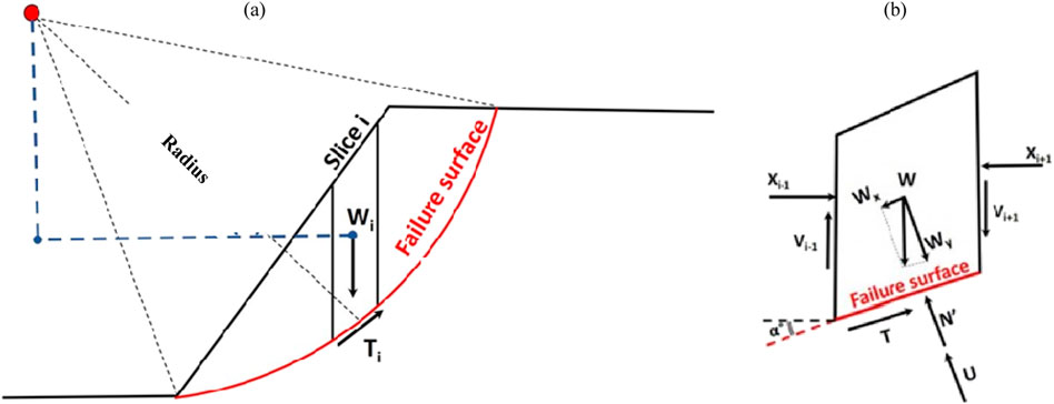
Figure 1. (A) Schematic representing: analysis of circular failure of slopes using Bishop’s method of slices. (B) Forces acting on a single slice: (i) the weight of the soil above the failure surface W, (ii) the interslice reactions from the adjacent slices X_i-1, X_i+1, V_i-1, V_i+1, (iii) the reaction of the stable ground which consists of a normal effective N′ and a shear component T, respectively, and (iv) the boundary water force U.

2.1.3 Jambu’s method

Janbu’s approach is suitable to non-circular soil mass failure. Similar to Bishop’s method, shear stress acting between the slices is ignored because horizontal forces should exist on the sides of each slice, and the normal force is assumed to act at the center of each slice’s base. Janbu’s corrected approach, which took into account the inter-slice shear force, was applied by Verma et al. (2013). The Janbu approach suggests that the interslice forces are normal. Equation 5 provides the Janbu expression for FoS.

$FoS=\frac{c^{\prime }l+\left(P-r_{u}l\right)\tan \left({\varphi }^{\prime }\right)\sec \left(\alpha \right)}{\sum W\sin \left(\alpha \right)}(5)$

Figure 2 depicts the slice approach for analyzing non-circular failures on slopes using Janbu’s method and the forces acting on a single slice. Researchers employed non-circular failure analysis as well as Janbu’s corrected approach for circular failure in slopes.

Figure 2

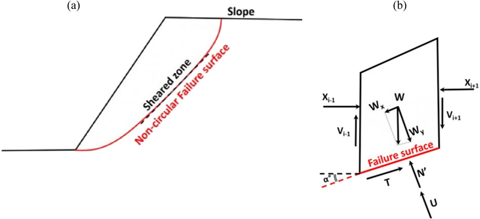
Figure 2. (A) Schematic representing: analysis of non-circular failure of slopes using Jambu’s method of slices. (B) Forces acting on a single slice: (i) the weight of the soil above the failure surface W, (ii) the interslice reactions from the adjacent slices X_i-1, X_i+1, V_i-1, V_i+1, (iii) the reaction of the stable ground which consists of a normal effective N′ and a shear component T, respectively, and (iv) the boundary water force U.

2.1.4 Lowe–Karafiath’s method

The primary purpose of Lowe–Karafiath’s Method (Lowe, 1960) is to analyze and assess the safety of slopes, embankments, and earth structures by calculating the factor of safety against potential sliding along a slip surface. In FoS computation, Lowe-Karafiath’s technique (Lowe, 1960) satisfies only force equilibrium. Lowe-Karafiath’s technique, like other methods, makes the assumption that the inclination of the interslice force is equal to the average of the inclinations of the slope surface (β) and the slice base (α), that is, $\theta =\frac{1}{2}\left(\alpha +\beta \right)$ where θ is the inclination of the interslice resultant force. Hence, the interslice forces can be expressed in Equation 6 as follows:

$T=E\tan \theta (6)$

2.1.5 Corps of engineers method

The Corps of Engineers approach is similar to Lowe-Karafiath’s method, with the exception of the assumption of interslice force inclination. The Corps of Engineers method is used to determine the FoS for slope stability. There are two possible approaches to assume the angle of the interslice resultant force using this method. Initially, it can be presumed that it is parallel to the ground, meaning that θ = β, where β represents the slope angle. Secondly, it can be equivalent to the average angle of slope between the critical shear surface’s entry and exit points.

2.1.6 Sarma’s method

Sarma’s Method Sarma (1973) is a well-established technique for determining the FoS for slope stability, especially in complex scenarios involving non-circular slip surfaces. Both of the equilibrium requirements are met by this approach (Abramson et al., 2002). Additionally, a linear Mohr-Coulomb expression (Equation 7) is assumed for the interslice force interaction.

$T=ch+E\tan \varphi (7)$

where, c and ϕ are the shear strength parameters, and h is the slice height.

2.1.7 Morgenstern-price method

The Morgenstern-Price method, which assumes the interslice force function, also fulfills both force and moment equilibriums. The interslice force inclination can vary with an arbitrary function (f(x)) as per the Morgenstern-Price approach (Morgenstern and Price, 1965) and presented in Equation 8:

$T=f\left(x\right)\cdot \lambda \cdot E(8)$

Where, λ = the scaling factor of the assumed function and f(x) = the interslice force function, which varies continuously through the slip surface. The approach proposes assuming any kind of force function, such as user-defined, half-sine, or trapezoidal. The base normal force (N) and the interslice forces (E, T) have the same relationships as those found in Janbu’s generalized technique. The interslice forces for a particular force function are calculated iteratively until F_f equals F_m in the Equations 9 and 10 (Nash, 1987).

$F_f=\frac{\sum \left[\left\{c^{\prime }l+\left(N-ul\right)\tan \left({\varphi }^{\prime }\right)\right\}\sec \left(\alpha \right)\right]}{\sum \left\{W-\left(T_2-T_1\right)\right\}\tan \left(\alpha \right)+\sum \left(E_2-E_1\right)}(9)$

$F_m=\frac{\sum \left(c^{\prime }l+\left(N-ul\right)\tan \left({\varphi }^{\prime }\right)\right)}{\sum W\sin \left(\alpha \right)}(10)$

2.1.8 Spencer’s method

Spencer’s approach is identical to the Morgenstern-Price method, with the exception of the assumption for interslice forces. For interslice forces, a constant inclination is assumed, and the FoS is calculated for both equilibrium (Spencer, 1967). Using this approach, the interslice shear force is associated with Equation 11:

$T=E\tan \theta (11)$

2.1.9 Friction circle method

The friction circle method is part of the broader category of limit equilibrium methods used for analyzing slope stability. This method divides the slip surface into vertical slices and evaluates forces and moments for each slice to determine equilibrium (Terzaghi et al., 1996). It calculates the FoS by comparing resisting forces, derived from soil friction along the slip surface, to driving forces. The method is particularly useful for preliminary assessments of slopes with cohesive soils, where circular failure surfaces are likely. While it simplifies calculations, it assumes uniform soil properties and a circular failure surface, which may not always reflect real conditions.

2.1.10 Taylor’s method

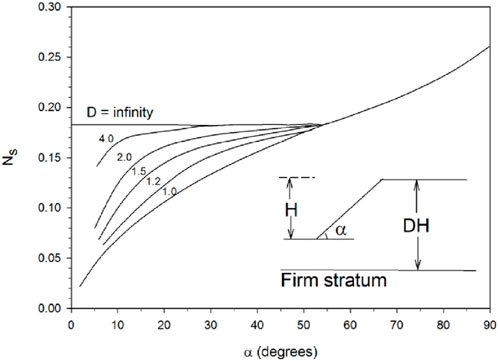
Taylor’s method is applicable for circular failure of the soil mass (Taylor, 1937). The assumption that soils are homogeneous and isotropic is incorrect in practice (Sakellariou and Ferentinou, 2005). Researchers previously used Taylor’s slope stability chart to estimate the factor of safety of slopes having simple geometry with homogenous and isotropic soil properties in clays under single-value undrained shear strength (Javankhoshdel and Bathurst, 2014; Liu et al., 2022). Taylor (1937) developed charts for calculating the factor of safety for simple slopes of cohesive-frictional (c-ϕ) shear strength soils. The disadvantages of Taylor’s chart include the requirement for repeated processes to determine the FoS. Equation 12 can be used to compute the FoS. Taylor’s slope stability chart is shown in Figure 3.

$FoS=\frac{S_u}{\gamma H{N}_s}(12)$

Figure 3

Figure 3. Schematic representing Taylor’s slope stability chart for cohesive soils.

where the depth factor (D) and slope angle (α) determine the stability number (N_s). In Figure 3, “H” represents the slope’s height and “DH” the hard stratum’s depth from the slope crest. It is generally accepted that “H” and “α” are deterministic. Additionally, S_u, a lognormally distributed or random variable, and γ, a constant, or both, can be used to compute the probability of failure for lognormal distributions with uncorrelated random variables.

2.1.11 Linear surface method

The Linear Surface Failure Method, used for analyzing infinite slopes in granular soils, assumes a planar failure surface. It is particularly effective for evaluating stability in granular materials like sand where cohesion is minimal (Duncan et al., 2014). The method involves calculating the factor of safety (FS) by comparing the resisting forces (due to friction) to the driving forces (due to gravity). This approach simplifies analysis by assuming an infinite slope and a linear failure surface, making it suitable for preliminary assessments of steep slopes.

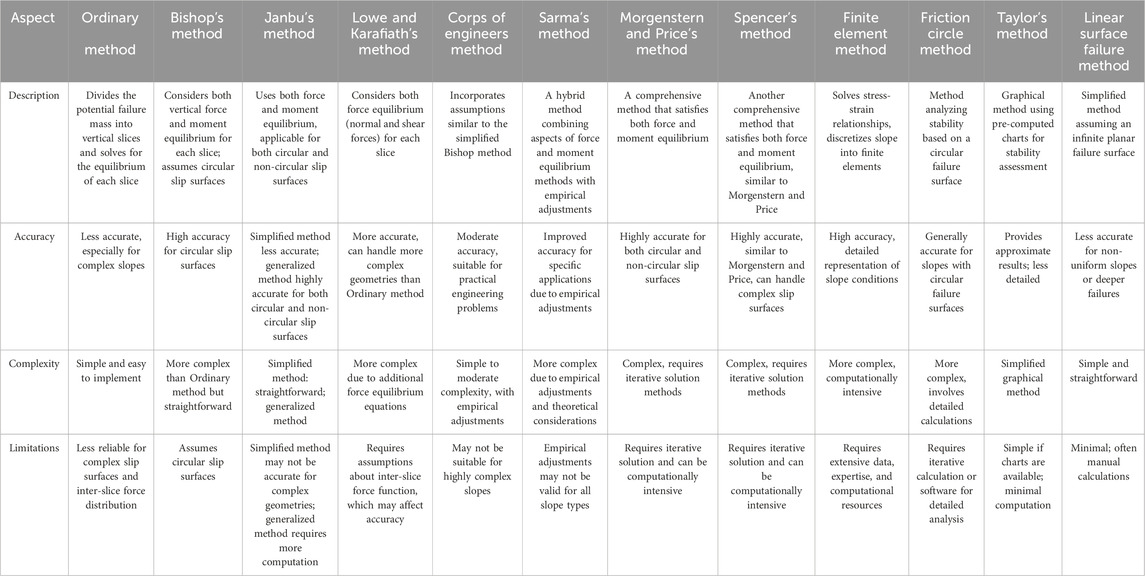
Table 2 contains detail comparison of various limit equilibrium methods used in slope stability analysis, including the Ordinary Method, Bishop’s method, Jambu’s method, Corps of Engineers method, Sarma’s method, Lowe and Karafiath’s method, Morgenstern and Price’s method, Spencer’s method, Finite element method, Taylor’s method, and Linear surface failure method.

Table 2

Table 2. Comparison of conventional slope stability methods.

2.2 Soft computing methods

Figure 4 displays the uses of soft computing methods in slope stability analysis over the past 20 years (2003–2022). The trend line is shown by the black dashed line, while the bars show the yearly number of studies. The Web of Science database provided the statistical data. After determining the relevance of the papers to the topic and using the search terms “soft computing method” and “slope stability analyses,” 159 publications from 2002 to 2022 were found. In comparison to 2019, the number of publications increased significantly in 2022. This demonstrates that the application of soft computing methods to slope stability issues has received more attention from researchers in recent years. It should be noted that many soft computing methods can be employed in a single article, resulting in a greater number of methods utilized than the number of papers reporting those research.

Figure 4

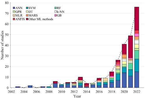
Figure 4. Number of machine learning research on slope stability conducted each year, with the trend line represented by the dashed line.

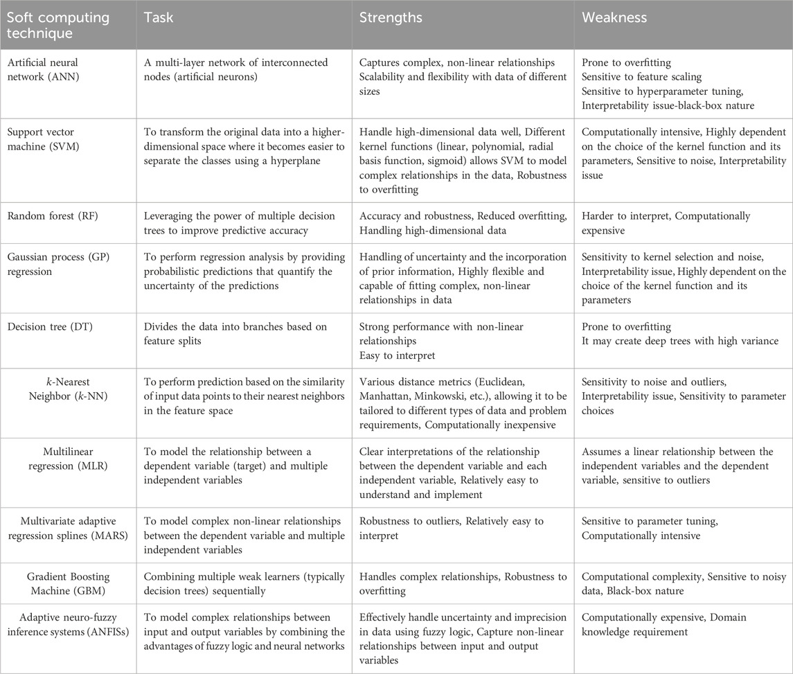
The majority of published works have examined related to slopes stability subjected to circular-type failure and stability of these slopes are based on slope geometry (i.e., H and β), shear strength of the geomaterial (i.e., c and ϕ), gravity (i.e., γ), and water condition (i.e., r_u). Soft computing/data mining methods based on historical/modeled data have been applied for two main purposes in these studies: (1) prediction of FoS, i.e., the output of these models is the FoS, and (2) prediction of slope stability (SS) status, i.e., the output of proposed models indicates the stability or instability of the slope. Several of these models are compared below in terms of FoS/SS and their performance metrics. Table 3 presents the comparison of these soft computing techniques highlighting their strengths and weakness in slope stability.

Table 3

Table 3. Brief comparison of different soft computing methods used in slope stability prediction.

2.2.1 Artificial neural network (ANN)

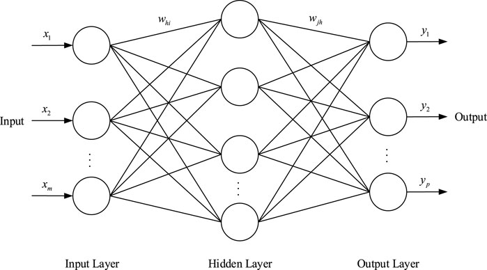
In the ANN mathematical model, neurons are regarded as processing elements or nodes. A network with input vectors x₁, x₂, … , x_m and output vectors y₁, y₂, … , y_p as shown in Figure 5, can be expressed in Equation 13 as follows:

$y_j=f_{output}\left[{\displaystyle \sum _{h=1}^k}{w}_{jh}{f}_{hidden}\left({\displaystyle \sum _{i=1}^m}{w}_{hi}{x}_i+w_{h0}\right)+w_{j0}\right](13)$

where f_hidden and f_output represent the respective transfer functions for the hidden and output layers. w_hi and w_jh represent the neuron weights of input neuron i to hidden neuron h and hidden neuron h to output neuron j, respectively. x_i is the i^th input unit; k is the number of neurons in the hidden layer; m is the number of input units; p is the number of output units; w_ho is the threshold (or bias) for neuron h; w_jo is the threshold for neuron j.

Figure 5

Figure 5. Typical architecture of a neural network.

Neural network models can be classified as feed forward or feedback based on their topology. The back propagation (BP) and radial basis function (RBF) algorithm models are commonly used in soft computing prediction models.

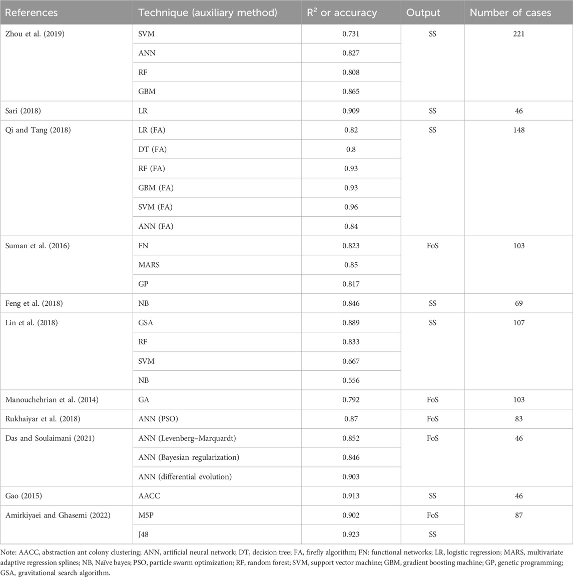
Zhou et al. (2019) employed ANN to predict slope stability, with a 0.827 accuracy. Similarly, Qi and Tang (2018) used ANN to predict slope stability and found an accuracy of 0.84.

2.2.2 Support vector machine (SVM)

The optimal classification hyper-plane problem with linear separability is the basis for the SVM method (Samui, 2008; Zhu and Zhang, 2004). Maximizing the training set interval is the algorithm’s objective. Nonnegative relaxation variables $\left({\xi }_n,n=1,2,...,k\right)$ are necessary for generalized optimum classifications under conditions that are not linearly separable. Then, the Equations 14, 15 present classification hyper-plane optimization problem:

$\underset{w,b}{\min }=\frac{{‖w‖}^2}{2}+C{\sum }_{i=1}^n{\xi }_i^2(14)$

which subject to

$\left\{\begin{array}{l}{y}_i\left(w\times x_i+b\right)\ge 1-{\xi }_i\\ {\xi }_i\ge 0,i=1,2,...,n\end{array}\right.(15)$

where $C\in \left(0,+\infty \right)$ is the parameter for penetration, $w$ is the normal vector, and $b$ is the hyper-plane’s bias. Through nonlinear transformations, the SVM algorithm can convert the input space into a high-dimensional space. The kernel function $K\left(x_i,x_j\right)=\mathrm{\Phi }\left(x_i\right)\times \mathrm{\Phi }\left(x_j\right)$ can be used to define the nonlinear transformation. There are four kernel functions, with the most popular being the radial basis function (RBF) kernel. The function of the radial basis function kernel is given in Equation 16:

$K\left(x_i,x_j\right)=\exp {\left(-\sigma ‖x_i-x_j‖\right)}^2(16)$

where $\sigma$ is the essential kernel parameter that specifies the kernel’s width, and $\sigma \in \left(0,1\right).$

The SVM for slope stability was applied by Lin et al. (Lin et al., 2018) with six typical slope parameters: pore water ratio, unit weight, cohesion, internal friction angle, slope angle, and slope height and found an accuracy of 0.6667.

2.2.3 Random forest (RF)

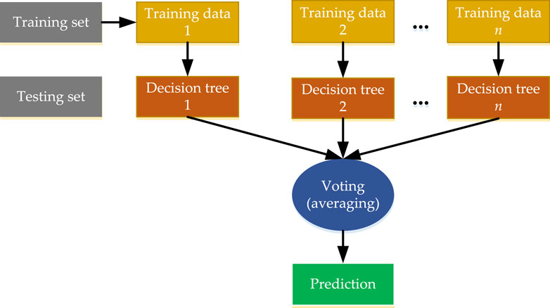
An ensemble learning technique called RF is used to address regression and classification issues. Breiman in 2001 developed a combinatorial classification method called the RF (Breiman, 2001). It is comprised of many decision-tree classification models $\mathrm{\Theta }\left\{h\left(X,k\right),k=1,2,...\right\}$, where the input vector and the parameter set is a random vector that is independently and identically distributed. The inconsistent results are decided by the voting process. The following is the main idea of RF: The original sample set is resampled to create numerous sample sets, each of which reflects the entirety of the training data for a given category tree. When each sample set evolves into a tree, m_try properties are selected at random from the M properties at each node. Once the purity of every node reaches its lowest point, one of the m_try attributes is chosen to mature. The generated n_tree trees can then be used to build the RF classifier, which can then be used to classify the newly data set. The number of votes by tree classifiers influences the classification result and presented in Equation 17 is:

$c=argma{x}_c\left(\frac{{\sum }_{k=1}^{n_{tree}}I\left(h\left(X,\mathrm{\Theta }k\right)=c\right)}{n_{tree}}\right)(17)$

where $c$ is the result of the classification and n_tree is the number of trees. Figure 6 depicts the RF functional architecture.

Figure 6

Figure 6. A random forest process’s typical architecture.

Zhou et al. (2019) found that the accuracy value was 0.808 after applying RF to 221 datasets for slope stability. In order to determine slope stability, Lin et al. (2018) employed RF on 132 datasets, yielding an accuracy of 0.83. In the same way, Qi and Tang (2018) used RF to analyze the soil slope stability of 148 slope instances and achieved an accuracy of 0.93.

2.2.4 Gaussian process regression (GPR)

Rasmussen’s hypothesis—that neighboring observations should to exchange information—forms the foundation of the GPR model (Rasmussen and Williams, 2006). A joint multivariate Gaussian distribution can be found for any finite number of the random variables in a gaussian process. Let a×b stand for the input and output domains, respectively, from which n uniformly and randomly distributed pairs (a_i, b_i) are taken. For regression, let $b\mathfrak{\subseteq }\mathfrak{R}$; then, a Gaussian process on a is distinct by the mean function $\mu :a\to \mathfrak{R}$ and a covariance function $k:a\times a\to \mathfrak{R}$. The main supposition of GP regression is that y is given as $b=f\left(a\right)+\xi$, where $\xi \sim N\left(0,{\sigma }^2\right)$. In GPR, for every input x, there is a corresponding random variable f(a), which is the value of the stochastic function f at that location. That is, In GPR, there is a corresponding random variable f(a)that represents the value of the stochastic function f at that specific position for each input x. In this work, it is assumed that the observational error n is normal independent and identically distributed, with a mean value of zero $\mu \left(a\right)=0$, a variance of ${\sigma }^2$ and f(a) drawn from the Gaussian process on a specified by k. This is given in Equation 18,

$B=\left(b_1,...,b_n\right)\sim N\left(0,K+{\sigma }^{2}I\right)(18)$

where K_ij = k (ai, aj) and I is the identity matrix. As $B/A\sim N\left(0,K+{\sigma }^{2}I\right)$ is normal, so is the conditional distribution of test labels given the training and test data of $\left(B/B,A,A*\right)$ . Then, one has $B*/B,A,A*\sim N\left(\mu ,\sum \right)$ where μ and ∑ are given in Equations 19 and 20:

$\mu =K\left(A*,A\right){\left[K\left(A,A\right)+{\sigma }^{2}I\right]}^{-1}B(19)$

$\sum =K\left(A*,A*\right)-{\sigma }^{2}I-K\left(A*,A\right){\left[K\left(A,A\right)+{\sigma }^{2}I\right]}^{-1}K\left(A,A*\right)(20)$

This is also true for the other values of K(A, A), K(A*, A), and K(A*, A*); here, A and B are the vectors of the training data and training data labels b_i, whereas A* is the vector of the test data. If there are n training data and n* test data, then K(A, A*) represents the n × n* matrix of covariance, which is evaluated at all pairs of training and test datasets. Tien Bui et al. (2019) used GPR for predicting slope stability FoS and found that the R² value is 0.9467.

2.2.5 Decision tree (DT)

DT addresses both regression and classification issues using a structure like a tree (Kardani et al., 2021; Pekel et al., 2020). Nodes in a DT model that have outgoing edges are called internal nodes, while nodes without any edges are called leaf nodes (leaves). DT models also use branches to connect the nodes. Classification trees and regression trees are the two forms of DTs. Classification trees divide data into two subsets according to class labels, and they keep doing this until a stopping criteria is reached. Another kind of DT used in machine learning to address regression issues is regression trees. They are used for predicting continuous output variables, as compared to classification trees, which are used to predict a discrete set of values. Regression trees split data into two groups and continue doing so until a stopping condition is met. DTs have numerous advantages, including ease of understanding and explanation (Witten and James, 2013). But DTs can be extremely sensitive. Minor adjustments to the input data can have considerable effects on the trees and the results (Witten and James, 2013). Because of their reliance on the greedy algorithm, DTs may occasionally fail in achieving a globally optimal outcome (Ben-Gal et al., 2014). A tree structure may effectively show the relationship between binary dependent variables and related independent variables, which is one of the advantages of DT analysis. Decision trees are hence a popular and effective data mining technique (Duch et al., 2004). Amirkiyaei and Ghasemi (2022) used J48 to assess the stability of slopes with 92.3% accuracy.

2.2.6 k-nearest neighbor (k-NN)

The k-NN approach is a well-known soft computing technique that is used to solve regression and classification issues. In the feature space, it is assumed that similar samples are frequently found near to one another (Peterson, 2009). The k-NN technique determines the k closest samples within the dataset for each sample point and computes their distance from the previous sample points. The samples that satisfy k with the smallest distances comprise the input data. The outcome of classification problems is class membership (labels). The majority class among the k closest samples is used to classify a sample. The sample is assigned to the closest class if k = 1. The average value of the closest samples in a regression issue is the output value (Mahmoodzadeh et al., 2022). The k-NN method’s quick and easy training process is one of its benefits. Furthermore, the k-NN method can reduce noise to some degree (Bhatia, 2010). But as k is a sensitive parameter, a smaller value could result in overfitting, while a bigger value could result in underfitting. Furthermore, processing costs might be high, particularly for large datasets (Bhatia, 2010). To ensure performance, hyperparameters must be properly chosen. Image recognition is one of the k-NN method’s application scenarios (Zhang et al., 2006; Homaeinezhad et al., 2012), text classification (Trstenjak et al., 2014; Tan, 2006), and recommendation system (Adeniyi et al., 2016). Huang et al. (2020) used k-NN algorithm for slope stability to achieve prediction accuracy up to 92.30%.

2.2.7 Multilinear regression (MLR)

The MLR, often known as multiple regression, is a simple machine learning technique that explains the relationship between two or more predictor variables and a response variable. The model is shown in Equation 21 (Pandey et al., 2022):

$y={\alpha }_0+{\alpha }_1\times x_1+{\alpha }_2\times x_2+...+{\alpha }_n\times x_n+\xi (21)$

where y is the dependent variable (output data), α₀ is the intercept or constant term, and α₁ to α_n are the coefficients of the independent variables (input data) x₁ to x_n, respectively. The MLR aims to minimize the sum of squared errors between the dependent variable’s actual values and its predicted values by estimating the values of the α coefficients. The fact that MLR can only take into account a linear relationship between the input and output data is one of its drawbacks. Chakraborty and Goswami (2017) used MLR to predict FoS of slope stability using 200 cases and found that R² is 0.847.

2.2.8 Multivariate adaptive regression splines (MARS)

MARS is a nonlinear regression approach that is used for classification and regression applications. MARS uses a collection of piecewise linear functions known as basis functions to model the relationship between several inputs and one output (Falae et al., 2021; Zhang and Goh, 2016). There are similarities between other basis functions, using the linear basis function as an example. The linear basis function Bi(x) can be defined in Equation 22 as three types:

(1) Constant values T (the intercept).

(2) A hinge function:

$B_i\left(x\right)=\max \left(0,x-T\right)(22)$

(3) A function of two or more hinge functions.

MARS model M can be expressed as a sum of basis functions given in Equation 23:

$M={\displaystyle \sum _{i=1}^t}{t}_i{B}_i\left(x\right)(23)$

where t_i is the constant coefficient. The model iteratively adds new functions after beginning with a single basis function. The algorithm chooses each hinge’s ideal location in a stage-by-stage, greedy fashion (Friedman and Roosen, 1995). Using a limited number of basis functions, MARS has the advantage of developing a straightforward model that captures intricate interactions between inputs and outputs. On the other hand, MARS might be affected by the initial basis function and stopping criteria selected. MARS is often used in credit scoring (Lee et al., 2006; Lee and Chen, 2005), and species distribution models (Leathwick et al., 2006) and also has applications in time series analysis (Lewis and Stevens, 1991). Liao and Liao (Liao et al., 2020) used MARS to predict FoS of slope stability with R² value is 0.8629.

2.2.9 Gradient boosting machine (GBM)

To increase prediction accuracy, GBM is an ensemble of weak prediction models, like DTs. GBM constructs the model step-by-step and, because it can maximize any differentiable loss function, has far wider applicability than previous boosting techniques. GBM is an accurate and effective technique that works well for both regression and classification issues. Web search ranking and ecology are two areas of research where GBM modeling has been widely applied. The benefits of GBM include its ability to handle mixed-type data naturally, its strong prediction ability, and its proficiency in handling output space outliers. In Civil Engineering, GBM has been employed for predicting hanging wall stability (Qi et al., 2018). Zhou et al. (2019) found that 0.865 was the accuracy after using GBM to 221 datasets for slope stability.

2.2.10 Adaptive neuro-fuzzy inference systems (ANFISs)

The ANFISs are a soft computing technique that combines ANNs with Takagi-Sugeno fuzzy inference systems (Jang, 1993; Jang, 1991; Mu’azu, 2023). The essential component is a collection of fuzzy rules—conditional statements that read, “if x is A, then y is B”—that are used to simulate a system’s input–output relationship. An ANFIS uses backpropagation and gradient descent methods to train a model in about five stages (Jang, 1993):

(1) Fuzzy sets are created from the input data by applying membership functions.

(2) The input and rules are used to calculate each rule’s firing strength.

(3) Weighted averaging is used to compute normalized firing strengths.

(4) The parameters and weights are optimized by adjusting the subsequent parameters.

(5) The total output is calculated by adding up all of the incoming signals.

ANFIS’s main benefit is its ability to express structured knowledge and nonlinearity (Jang, 1993). To train the model, ANFIS needs an adequate dataset; yet, choosing the right input-output data is far more important. Additionally, the number of input data increases exponentially with the number of fuzzy rules, thus raising the cost of computation and may effect a model’s performance (Al-Mahasneh et al., 2016). Mohamed et al. (2012) used ANFIS and obtained R² of 0.9997 to predict FoS with high accuracy compared with MLR.

Some other soft computing methods are sparse polynomial chaos expansion is based on polynomial chaos expansion and hybrid soft computing models for predicting slope stability.

The use of soft computing models for slope stability analysis offers distinct advantages in terms of accuracy, flexibility, and efficiency, particularly in addressing the complexities and uncertainties associated with real-world slope conditions. On the other hand, numerous studies have been undertaken in recent years to develop soft computing models for predicting slope stability status (see Table 3). For example, Zhou et al. (2019) used the gradient boosting machine (GBM) method to analyze slope stability and compared to the artificial neural network (ANN), random forest (RF) and support vector machine (SVM). It was found that the GBM has highest accuracy i.e., 0.865. Sari (2018) used binary logistic regression analysis as an alternative technique to predict stability condition of slopes with 90.9% accuracy. Accordingly, Qi and Tang (2018) used basic ensemble classifier consisting of six individual classifiers and majority voting as a combination method to improve analysis of slope stability. It is worthwhile to note that the coefficient of determination (R²)/accuracy in Table 4 ranges from 0.556 to 0.96. Although, these models have greatly improved our understanding; however, the performance and accuracy of the predictive models are not well interpreted, and the problem of slope stability is still far from being fully solved. Therefore, the issue of slope failure still posed considerable challenge for geotechnical professionals. The existing slope stability issues and damages caused by landslides, it is necessary to put forward the idea that more systematic and in-depth research should be carried out on predicting the slope stability. Consequently, there is a need for more accurate and reliable methods to predict slope stability. Soft computing methods provide powerful tools for tackling complex, uncertain, and imprecise problems. Their flexibility, adaptability, and robustness make them suitable for a wide range of applications. Soft computing techniques are known for their proficiency in non-linear modeling, and there is evidence in the literature from a number of technical and scientific fields that these techniques can establish correlations between desired outcomes and a variety of influencing parameters, whether those parameters have direct or indirect impacts (Asteris et al., 2022; Koopialipoor et al., 2019). However, choosing a suitable soft computing model is challenging for the reasons listed below: (a) Inadequate modeling and validation; (b) models in use not being able to identify the precise global optimum; (c) problems with overfitting, etc. However, the challenges related to computational cost, interpretability, and data dependence must be carefully managed to fully leverage their potential.

Table 4

Table 4. Summary of soft computing methods used for slope stability.

3 Discussion

Slope instability poses severe risks to infrastructure, communities, and the environment. Prediction of slope stability is of primary concern in identifying terrain that is susceptible to landslides and mitigating the damages caused by landslides (Rukhaiyar et al., 2018; Alimohammadlou et al., 2014). It is difficult to accurately predict the stability of a slope due to the fact that it is dependent on a number of geotechnical and physical factors. Furthermore, the interactions between these factors are complex and “often difficult to describe mathematically” (Xue, 2017; Lu and Rosenbaum, 2003).

Several methods have been proposed to analyze or predict slope stability, among which are Limit Equilibrium (LE) Methods (Thiebes et al., 2014; Verma et al., 2013) and numerical methods [e.g., finite element method (FEM)] (Cai and Ugai, 2004; Dawson et al., 1999; Griffiths and Lane, 1999) are the most widely employed methods (Xue, 2017; Liu et al., 2014). Empirical equations (Bye and Bell, 2001; Taheri and Tani, 2010) and limit analysis approaches based on lower and upper bound theorems (Chen and Baladi, 1985) are other methods. All of the methods mentioned above, however, have some drawbacks. The LEMs, for example, cannot reflect the slip surfaces’ actual stress conditions (Lechman and Griffiths, 2000), and as a result of simplifying assumptions, their accuracy is compromised (Sakellariou and Ferentinou, 2005). The numerical methods are time-consuming, and their accuracy is strongly reliant on correct geotechnical and physical parameter estimation (Feng et al., 2018).

Slope stability analysis poses challenges due to limited information, data, and site specificity; thus, soft computing models prove to be a viable tool for problem solutions. Soft computing models have an advantage over conventional statistical and empirical relationships in that they can perform even in cases where there is no prior relationship between the predictors and predicted variables. It is important to note that a large number of researchers have worked extensively to develop numerous soft computing models, the effectiveness of which depends on a number of variables that were thoroughly addressed in this article. However, several performance measures, which depend on (i) input parameters, (ii) slope conditions, (iii) number of data points and many other factors, are typically used to determine the suitability of soft computing models. Soft computing techniques seem to be developing as useful techniques for assessing a variety of issues that are challenging to resolve using conventional methods. Nevertheless, there are certain difficulties when applying soft computing to slope stability problems because of (i) the scarcity of data in certain studies that are site- and location-specific, (ii) model underfitting and overfitting, and (iii) the likelihood of misfitting data, which could lead to anecdotal results because soft computing models are case- and site-specific. Modeling techniques are classified based on colors, with white-, black-, and grey-box models used for three levels of prior information (Giustolisi et al., 2007). Black-box models (e.g., ANN, SVM, etc.) are data-driven or regressive systems whose functional form of relationships between model variables is unknown and must be predicted. Black-box models rely on data to map the relationships between model inputs and outputs, rather than determining a suitable structure for the model input-output interactions. However, grey-box models (e.g., gene expression programming and evolutionary polynomial regression) are conceptual systems from which the mathematical structure of the model may be concluded, allowing additional information about the system’s behavior to be resolved. White-box models (i.e., TAN, REPT, RT, and C4.5 decision tree) are systems that openly demonstrate the relationship between input and output parameters. Figure 7 depicts the above classification, with the higher the physical knowledge used during model building, the better the physical interpretation of the phenomenon that the model provides to the user.

Figure 7

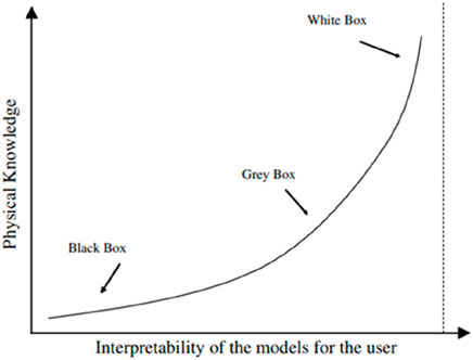
Figure 7. Graphical classifications of soft computing modeling techniques [modified from Giustolisi et al., (2007))].

Most of soft computing methods have not been able to realize their full potential in engineering applications due to their “black-box” nature and lack of interpretability. These models can be used by the user to rapidly evaluate and predict the slope stability and consequences. Based on literature reviews, these techniques have been effectively used to tackle several complex engineering issues in a variety of fields, although their use in geotechnical engineering is limited. The predictive models’ accuracy can be interpreted poorly, as they do not fully address the issue of slope stability or fully interpret the contribution of influencing parameters. Therefore, evaluating slope stability and determining the impact of influencing factors remain a considerable challenge for geotechnical professionals. It is critical to develop the idea of doing more systematic and in-depth study on predicting slope stability and interpreting the impact of influencing parameters. Therefore, in order to improve the effectiveness of these approaches, more thorough and in-depth research on soft computing models must be conducted.

4 Conclusion and future prospect

This paper focuses on conventional methods that have been in use for many years. Recent advancements in geotechnical engineering and soft computing models for slope stability adaptability and feasibility have also been widely studied. In literature review it was concluded that the majority of soft computing models are easier to use, time-saving, and are more successful than conventional methods. Furthermore, the problems associated with slope stability in geotechnical engineering have evolved over time due to a variety of factors that make them difficult to model numerically and solve using conventional methods. Soft computing methods have been frequently employed in slope stability analysis, yielding promising results. With the availability of numerous open-source soft computing libraries, it has become easier for researchers to access. Although, these models have substantially improved our understanding; however, the performance and accuracy of the predictive models are not well interpreted, and the problem of slope stability is still far from being fully solved. Therefore, the issue of slope failure still posed considerable challenge for geotechnical professionals. The existing slope stability issues and damages caused by landslides, it is necessary to put forward the idea that more systematic and in-depth research should be carried out on predicting the slope stability. Consequently, there is a need for more accurate and reliable methods to predict slope stability. Furthermore, one of the primary issues with the most of the soft computing methods—with the exception of genetic programming and logistic regression—is that they are black-box. This indicates that they do not provide a transparent model that illustrates how input and output parameters relate to one another. In fact, the “black-box” aspect and lack of interpretability of most of soft computing techniques have hindered them from reaching their full potential in engineering applications. However, soft computing methods such as tree augmented naive-bayes (TAN), reduced error pruning tree (REPT), random tree (RT), logistic model tree (LMT), and C4.5 decision tree are regarded as a “white-box” that clearly displays the relationship between input and output parameters. These models can be used by the user to rapidly evaluate and predict the slope stability and consequences. It is therefore suggested that in the future, an effort be made to develop robust and transparent models for evaluating the stability of slopes that are subject to circular mode failures with improved prediction accuracy.

Author contributions

FA: Conceptualization, Data curation, Formal Analysis, Investigation, Methodology, Writing–original draft, Writing–review and editing. X-WT: Conceptualization, Funding acquisition, Methodology, Supervision, Validation, Writing–review and editing. MA: Formal Analysis, Investigation, Validation, Writing–review and editing. TN: Funding acquisition, Investigation, Project administration, Resources, Supervision, Validation, Writing–review and editing. YG: Funding acquisition, Methodology, Supervision, Validation, Writing–review and editing.

Funding

The author(s) declare that financial support was received for the research, authorship, and/or publication of this article. The work was supported by the National Key Research and Development Plan of China under Grant No. 2021YFB2600703.

Conflict of interest

The authors declare that the research was conducted in the absence of any commercial or financial relationships that could be construed as a potential conflict of interest.

Publisher’s note

All claims expressed in this article are solely those of the authors and do not necessarily represent those of their affiliated organizations, or those of the publisher, the editors and the reviewers. Any product that may be evaluated in this article, or claim that may be made by its manufacturer, is not guaranteed or endorsed by the publisher.

Abbreviations

AACC, abstraction ant colony clustering; ANFIS, adaptive neuro-fuzzy inference system; ANN, artificial neural network; DT, decision tree; FoS, factor of safety; FA, firefly algorithm; FN, functional network; GB, gradient boosting; GPR, Gaussian process regression; GBM, gradient boosting machine; GP, genetic programming; GSA, gravitational search algorithm; k-NN, k-nearest neighbor; LDC, linear discriminant classifier; LE limit equilibrium; MARS, multivariate adaptive regression splines; MLR, multilinear regression; NB, Naïve bayes; PSO, particle swarm optimization; R², coefficient of determination; RF, random forest; SVM, support vector machine; r_u, Pore pressure ratio; β, Slope angle; G_f , failure gravity; G_i, real-world gravity; H, Slope height; c or c′, Cohesion; ϕ or ϕ′, angle of internal friction; γ, Unit weight.

References

Abramson, L. W., Lee, T. S., Sharma, S., and Boyce, G. (2002). Slope stability concepts. Slope stabilization and stabilization methods. United States: John Wiley and Sons, Inc. published by John Willey & Sons.

Google Scholar

Adeniyi, D. A., Wei, Z., and Yongquan, Y., Automated web usage data mining and recommendation system using K-Nearest Neighbor (KNN) classification method., 2016. 12(1) 90–108. doi:10.1016/j.aci.2014.10.001

CrossRef Full Text | Google Scholar

Alimohammadlou, Y., Najafi, A., and Gokceoglu, C. (2014). Estimation of rainfall-induced landslides using ANN and fuzzy clustering methods: a case study in Saeen Slope, Azerbaijan province, Iran. Catena 120, 149–162. doi:10.1016/j.catena.2014.04.009

CrossRef Full Text | Google Scholar

Al-Mahasneh, M., Aljarrah, M., Rababah, T., and Alu’datt, M. (2016). Application of hybrid neural fuzzy system (ANFIS) in food processing and technology. Appl. hybrid neural fuzzy Syst. (ANFIS) food Process. Technol. 8, 351–366. doi:10.1007/s12393-016-9141-7

CrossRef Full Text | Google Scholar

Amirkiyaei, V., and Ghasemi, E. (2022). Stability assessment of slopes subjected to circular-type failure using tree-based models. Int. J. Geotechnical Eng. 16 (3), 301–311. doi:10.1080/19386362.2020.1862538

CrossRef Full Text | Google Scholar

Asteris, P. G., Lourenço, P. B., Roussis, P. C., Adami, C. E., Armaghani, D. J., Cavaleri, L., et al. (2022) Revealing the nature of metakaolin-based concrete materials using artificial intelligence techniques, 322.126500

CrossRef Full Text | Google Scholar

Bathe, K.-J. (2006). Finite element procedures. Klaus-Jurgen Bathe.

Google Scholar

Belytschko, T., Liu, W. K., Moran, B., and Elkhodary, K. (2014). Nonlinear finite elements for continua and structures. United States: John Wiley & Sons.

Google Scholar

Ben-Gal, I., Dana, A., Shkolnik, N., and Singer, G., Efficient construction of decision trees by the dual information distance method. , 2014. 11(1) 133–147. doi:10.1080/16843703.2014.11673330

CrossRef Full Text | Google Scholar

Bhatia, N. J., Survey of nearest neighbor techniques. 2010.

Google Scholar

Bishop, A. W. (1955). The use of the slip circle in the stability analysis of slopes. Geotechnique 5 (1), 7–17. doi:10.1680/geot.1955.5.1.7

CrossRef Full Text | Google Scholar

Bishop, A. W., and Morgenstern, N. (1960). Stability coefficients for earth slopes. Geotechnique 10 (4), 129–153. doi:10.1680/geot.1960.10.4.129

CrossRef Full Text | Google Scholar

Breiman, L. (2001). Random forests. Mach. Learn. 45 (1), 5–32. doi:10.1023/a:1010933404324

CrossRef Full Text | Google Scholar

Bye, A., and Bell, F. (2001). Stability assessment and slope design at Sandsloot open pit, South Africa. Int. J. Rock Mech. Min. Sci. 38 (3), 449–466. doi:10.1016/s1365-1609(01)00014-4

CrossRef Full Text | Google Scholar

Cai, F., and Ugai, K. (2004). Numerical analysis of rainfall effects on slope stability. Int. J. Geomechanics 4 (2), 69–78. doi:10.1061/(asce)1532-3641(2004)4:2(69)

CrossRef Full Text | Google Scholar

Chakraborty, A., and Goswami, D. (2017). Predict. slope Stab. using multiple linear Regres. (MLR) Arabian Journal of Geosciences 10, 1–11. doi:10.1007/s12517-017-3167-x

CrossRef Full Text

Chen, W.-F., and Baladi, G. Y. (1985). Soil plasticity: theory and implementation. Elsevier.

Google Scholar

Cheng, Y. M., Lansivaara, T., and Wei, W. (2007). Two-dimensional slope stability analysis by limit equilibrium and strength reduction methods. Comput. Geotech. 34 (3), 137–150. doi:10.1016/j.compgeo.2006.10.011

CrossRef Full Text | Google Scholar

Choobbasti, A., Farrokhzad, F., and Barari, A. (2009). Prediction of slope stability using artificial neural network (case study: noabad, Mazandaran, Iran). Predict. slope Stab. using Artif. neural Netw. (case study Noabad, Mazandaran, Iran). Arab J Geosci 2 (4), 311–319. doi:10.1007/s12517-009-0035-3

CrossRef Full Text | Google Scholar

Cousins, B. F. (1978). Stability charts for simple earth slopes. J. Geotechnical Eng. Div. 104 (2), 267–279. doi:10.1061/ajgeb6.0000585

CrossRef Full Text | Google Scholar

Das, R., and Soulaimani, A. (2021). Non-deterministic methods and surrogates in the design of rockfill dams. Appl. Sci. 11 (8), 3699. doi:10.3390/app11083699

CrossRef Full Text | Google Scholar

Dawson, E., Roth, W. H., and Drescher, A. (1999). Slope stability analysis by strength reduction. Géoteclinique 49 (6), 835–840. doi:10.1680/geot.1999.49.6.835

CrossRef Full Text | Google Scholar

Duch, W., Setiono, R., and Zurada, J. M. (2004). Computational intelligence methods for rule-based data understanding. Proc. IEEE 92 (5), 771–805. doi:10.1109/jproc.2004.826605

CrossRef Full Text | Google Scholar

Duncan, J. M. (1996). State of the art: limit equilibrium and finite-element analysis of slopes. J. Geotechnical Eng. 122 (7), 577–596. doi:10.1061/(asce)0733-9410(1996)122:7(577)

CrossRef Full Text | Google Scholar

Duncan, J. M., Wright, S. G., and Brandon, T. L. (2014). Soil strength and slope stability. John Wiley & Sons.

Google Scholar

Ebid, A. M., Onyelowe, K. C., and Arinze, E. E. (2021a). Estimating the ultimate bearing capacity for strip footing near and within slopes using AI. (GP, ANN, EPR) Tech. 2021 (1), 3267018. doi:10.1155/2021/3267018

CrossRef Full Text | Google Scholar

Ebid, A. M. J. G., and Engineering, G., 35 Years of (AI) in geotechnical engineering: state of the art. 2021b. 39(2). 637–690.

CrossRef Full Text | Google Scholar

Falae, P. O., Agarwal, E., Pain, A., Dash, R. K., and Kanungo, D. P. (2021). A data driven Effic. Framew. probabilistic slope Stab. analysis Pakhi landslide, Garhwal Himalaya 130, 1–15. doi:10.1007/s12040-021-01641-y

CrossRef Full Text

Fellenius, W. (1936). Calculation of the stability of earth dams. Proc. 2nd. Congr. Large Dams 4, 445–462.

Google Scholar

Feng, X., Li, S., Yuan, C., Zeng, P., and Sun, Y. (2018). Prediction of slope stability using naive Bayes classifier. KSCE J. Civ. Eng. 22 (3), 941–950. doi:10.1007/s12205-018-1337-3

CrossRef Full Text | Google Scholar

Friedman, J. H., and Roosen, C. B. (1995). An introduction to multivariate adaptive regression splines. Thousand Oaks, CA: Sage Publications Sage CA, 197–217.

Google Scholar

Gao, W. (2015). Stability analysis of rock slope based on an abstraction ant colony clustering algorithm. Environ. Earth Sci. 73 (12), 7969–7982. doi:10.1007/s12665-014-3956-4

CrossRef Full Text | Google Scholar

Giustolisi, O., Doglioni, A., Savic, D., and Webb, B., A multi-model approach to analysis of environmental phenomena. , 2007. 22(5). 674–682. doi:10.1016/j.envsoft.2005.12.026

CrossRef Full Text | Google Scholar

Griffiths, D., and Lane, P. (1999). Slope stability analysis by finite elements. Geotechnique 49 (3), 387–403. doi:10.1680/geot.1999.49.3.387

CrossRef Full Text | Google Scholar

Hassan, M. A., Ismail, M. A. M., and Shaalan, H. H. (2022). Numerical modeling for the effect of soil type on stability of embankment. Civ. Eng. J. 7, 41–57. doi:10.28991/cej-sp2021-07-04

CrossRef Full Text | Google Scholar

Homaeinezhad, M. R., Atyabi, S., Tavakkoli, E., Toosi, H., Ghaffari, A., and Ebrahimpour, R. (2012). ECG arrhythmia recognition via a neuro-SVM–KNN hybrid classifier with virtual QRS image-based geometrical features. Expert Syst. Appl. 39 (2), 2047–2058. doi:10.1016/j.eswa.2011.08.025

CrossRef Full Text | Google Scholar

Huang, S., Huang, M., and Lyu, Y. J., An improved KNN-based slope stability prediction model. , 2020. 2020(1): p. 8894109, doi:10.1155/2020/8894109

CrossRef Full Text | Google Scholar

Hunter, J. H., and Schuster, R. L. (1971). Chart solutions for analysis of earth slopes. Highw. Res. Rec., 345.

Google Scholar

Janbu, N. (1968). Slope stability computations, soil mechanics and foundation engineering report. Trondheim: Technical University of Norway.

Google Scholar

Jang, J.-S. J. I. (1993). ANFIS: adaptive-network-based fuzzy inference system. ANFIS adaptive-network-based fuzzy inference Syst. 23 (3), 665–685. doi:10.1109/21.256541

CrossRef Full Text | Google Scholar

Jang, J.-S. R. (1991) “Fuzzy modeling using generalized neural networks and Kalman filter algorithm,” in Proceedings of the ninth National conference on Artificial intelligence, 2.

Google Scholar

Javankhoshdel, S., and Bathurst, R. J. (2014). Simplified probabilistic slope stability design charts for cohesive and cohesive-frictional (c-ϕ) soils. Can. Geotechnical J. 51 (9), 1033–1045. doi:10.1139/cgj-2013-0385

CrossRef Full Text | Google Scholar

Kardani, N., Zhou, A., Nazem, M., and Shen, S. L., Improved prediction of slope stability using a hybrid stacking ensemble method based on finite element analysis and field data, 2021. 13(1) 188–201. doi:10.1016/j.jrmge.2020.05.011

CrossRef Full Text | Google Scholar

Kaur, A., and Sharma, R. (2016). Technology. Slope Stab. Anal. Tech. a Rev. 1 (4), 52–57.

Google Scholar

Koopialipoor, M., Tootoonchi, H., Jahed Armaghani, D., Tonnizam Mohamad, E., and Hedayat, A. (2019). Application of deep neural networks in predicting the penetration rate of tunnel boring machines. Bull. Eng. Geol. Environ. 78, 6347–6360. doi:10.1007/s10064-019-01538-7

CrossRef Full Text | Google Scholar

Leathwick, J., Elith, J., and Hastie, T. J. E. m. (2006). Comparative performance of generalized additive models and multivariate adaptive regression splines for statistical modelling of species distributions. Ecol. Modell. 199 (2), 188–196. doi:10.1016/j.ecolmodel.2006.05.022

CrossRef Full Text | Google Scholar

Lechman, J., and Griffiths, D. (2000). “Analysis of the progression of failure of earth slopes by finite elements,” in Slope stability, 250–265.

CrossRef Full Text | Google Scholar

Lee, T.-S., and Chen, I.-F. J. E. S. w.a. (2005). A two-stage hybrid credit scoring model using artificial neural networks and multivariate adaptive regression splines. Expert Syst. Appl. 28 (4), 743–752. doi:10.1016/j.eswa.2004.12.031

CrossRef Full Text | Google Scholar

Lee, T.-S., Chiu, C. C., Chou, Y. C., and Lu, C. J., Mining the customer credit using classification and regression tree and multivariate adaptive regression splines. , 2006. 50(4) 1113–1130. doi:10.1016/j.csda.2004.11.006

CrossRef Full Text | Google Scholar

Lewis, P. A., and Stevens, J. G. J. J. o.t.A. S. A. (1991). Nonlinear modeling of time series using multivariate adaptive regression splines (MARS). J. Am. Stat. Assoc. 86 (416), 864–877. doi:10.2307/2290499

CrossRef Full Text | Google Scholar

Liao, Z., and Liao, Z. J. O. G., Slope stability evaluation using backpropagation neural networks and multivariate adaptive regression splines. , 2020. 12(1) 1263–1273. doi:10.1515/geo-2020-0198

CrossRef Full Text | Google Scholar

Lin, Y., Zhou, K., and Li, J. (2018). Prediction of slope stability using four supervised learning methods. IEEE Access 6, 31169–31179. doi:10.1109/access.2018.2843787

CrossRef Full Text | Google Scholar

Liu, L.-L., Zhang, P., Zhang, S. H., Li, J. Z., Huang, L., Cheng, Y. M., et al. (2022). Efficient evaluation of run-out distance of slope failure under excavation. Eng. Geol. 306, 106751. doi:10.1016/j.enggeo.2022.106751

CrossRef Full Text | Google Scholar

Liu, Z., Shao, J., Xu, W., Chen, H., and Zhang, Y. (2014). An extreme learning machine approach for slope stability evaluation and prediction. Nat. hazards 73 (2), 787–804. doi:10.1007/s11069-014-1106-7

CrossRef Full Text | Google Scholar

Lowe, J. (1960). “Stability of earth dams upon drawdown,” in Proc. 1st Pan American conference on soil (Mexico City: Mechanics and Foundation Engineering).

Google Scholar

Lu, P., and Rosenbaum, M. (2003). Artificial neural networks and grey systems for the prediction of slope stability. Nat. Hazards 30 (3), 383–398. doi:10.1023/b:nhaz.0000007168.00673.27

CrossRef Full Text | Google Scholar

Mahmoodzadeh, A., Mohammadi, M., Farid Hama Ali, H., Hashim Ibrahim, H., Nariman Abdulhamid, S., and Nejati, H R. (2022). Prediction of safety factors for slope stability: comparison of machine learning techniques. Nat. Hazards, 1–29.

CrossRef Full Text | Google Scholar

Manouchehrian, A., Gholamnejad, J., and Sharifzadeh, M. (2014). Development of a model for analysis of slope stability for circular mode failure using genetic algorithm. Environ. Earth Sci. 71 (3), 1267–1277. doi:10.1007/s12665-013-2531-8

CrossRef Full Text | Google Scholar

Matsui, T., and San, K.-C. J. S., Finite element slope stability analysis by shear strength reduction technique, 1992. 32(1) 59–70. doi:10.3208/sandf1972.32.59

CrossRef Full Text | Google Scholar

Mehmood, E., Rashid, I., Ahmed, F., Farooq, K., Tufail, A., and Ebid, A. M. (2022). Hydrogeotechnical predictive approach for rockfall mountain hazard using elastic modulus and peak shear stress at soil–rock interface in dry and wet phases at KKH Pakistan. Sustainability 14 (24), 16740. doi:10.3390/su142416740

CrossRef Full Text | Google Scholar

Mohamed, T., Kasa, A., and Mukhlisin, M. J. T., Prediction of slope stability using statistical method and fuzzy logic. 2012. 2(4): p. 68–73.

CrossRef Full Text | Google Scholar

Morgenstern, N. u., and Price, V. E. (1965). The analysis of the stability of general slip surfaces. Geotechnique 15 (1), 79–93. doi:10.1680/geot.1965.15.1.79

CrossRef Full Text | Google Scholar

Mu’azu, M. A. (2023). Enhancing slope stability prediction using fuzzy and neural frameworks optimized by metaheuristic science. Math. Geosci. 55 (2), 263–285. doi:10.1007/s11004-022-10029-7

CrossRef Full Text | Google Scholar

Nash, D. (1987). A comprehensive review of limit equilibrium methods of slope stability analysis. New York, NY: John Wiley, 11–75.

Google Scholar

Onyelowe, K. C., Ebid, A. M., Mahdi, H. A., and Baldovino, J. A. (2023c). Selecting the safety and cost optimized geo-stabilization technique for soft clay slopes. Civ. Eng. J. 9 (2), 453–464. doi:10.28991/cej-2023-09-02-015

CrossRef Full Text | Google Scholar

Onyelowe, K. C., Ebid, A. M., Ramani Sujatha, E., Fazel-Mojtahedi, F., Golaghaei-Darzi, A., Kontoni, D. P. N., et al. (2023b). Extensive overview of soil constitutive relations and applications for geotechnical engineering problems. Heliyon 9 (3), e14465. doi:10.1016/j.heliyon.2023.e14465

PubMed Abstract | CrossRef Full Text | Google Scholar

Onyelowe, K. C., Mojtahedi, F. F., Ebid, A. M., Rezaei, A., Osinubi, K. J., Eberemu, A. O., et al. (2023a). Selected AI optimization techniques and applications in geotechnical engineering. Cogent Eng. 10 (1), 2153419. doi:10.1080/23311916.2022.2153419

CrossRef Full Text | Google Scholar

Onyelowe, K. C., Sujatha, E. R., Aneke, F. I., and Ebid, A. M. (2022). Solving geophysical flow problems in Luxembourg: SPH constitutive review. Cogent Eng. 9 (1), 2122158. doi:10.1080/23311916.2022.2122158

CrossRef Full Text | Google Scholar

Pandey, V. H. R., Kainthola, A., Sharma, V., Srivastav, A., Jayal, T., and Singh, T. N. (2022). Deep learning models for large-scale slope instability examination in Western Uttarakhand, India. Environ. Earth Sci. 81 (20), 487. doi:10.1007/s12665-022-10590-8

CrossRef Full Text | Google Scholar

Pekel, E. J. T., and Climatology, A., Estimation of soil moisture using decision tree regression. 2020. 139(3-4): p. 1111–1119.

CrossRef Full Text | Google Scholar

Peterson, L. E. J. S., K-nearest neighbor. , 2009. 4(2): p. 1883, doi:10.4249/scholarpedia.1883

CrossRef Full Text | Google Scholar

Pourkhosravani, A., and Kalantari, B. J. (2011) A review of current methods for slope stability evaluation, 16, 1245–1254.

Google Scholar

Qi, C., Fourie, A., Ma, G., Tang, X., and Du, X. (2018). Comparative study of hybrid artificial intelligence approaches for predicting hangingwall stability. J. Comput. Civ. Eng. 32 (2), 04017086. doi:10.1061/(asce)cp.1943-5487.0000737

CrossRef Full Text | Google Scholar

Qi, C., and Tang, X. (2018). Slope stability prediction using integrated metaheuristic and machine learning approaches: a comparative study. Comput. & Industrial Eng. 118, 112–122. doi:10.1016/j.cie.2018.02.028

CrossRef Full Text | Google Scholar

Rasmussen, C., and Williams, C. (2006) Gaussian processes for machine learning, 38. Cambridge, MA, USA: The MIT Press, 715–719.

Google Scholar

Rukhaiyar, S., Alam, M., and Samadhiya, N. (2018). A PSO-ANN hybrid model for predicting factor of safety of slope. Int. J. Geotechnical Eng. 12 (6), 556–566. doi:10.1080/19386362.2017.1305652

CrossRef Full Text | Google Scholar

Sakellariou, M., and Ferentinou, M. (2005). A study of slope stability prediction using neural networks. Geotechnical & Geol. Eng. 23 (4), 419–445. doi:10.1007/s10706-004-8680-5

CrossRef Full Text | Google Scholar

Samui, P. (2008). Slope stability analysis: a support vector machine approach. Environ. Geol. 56 (2), 255–267. doi:10.1007/s00254-007-1161-4

CrossRef Full Text | Google Scholar

Sari, M. (2018). “Stability analysis of slopes prone to circular failures using logistic regression,” in Conference of the arabian journal of geosciences (Springer).

CrossRef Full Text | Google Scholar

Sarma, S. K. (1973). Stability analysis of embankments and slopes. Geotechnique 23 (3), 423–433. doi:10.1680/geot.1973.23.3.423

CrossRef Full Text | Google Scholar

Singh, P., Kumar, D., and Samui, P. (2020). Reliability analysis of rock slope using soft computing techniques. Jordan J. Civ. Eng. 14 (1).

Google Scholar

Spencer, E. (1967). A method of analysis of the stability of embankments assuming parallel inter-slice forces. Geotechnique 17 (1), 11–26. doi:10.1680/geot.1967.17.1.11

CrossRef Full Text | Google Scholar

Sternik, K. J. C. T. Ś., Comparison of slope stability predictions by gravity increase and shear strength reduction methods. 2013. 110(1-Ś) 121--130.

Google Scholar

Suman, S., Khan, S. Z., Das, S. K., and Chand, S. K. (2016). Slope stability analysis using artificial intelligence techniques. Nat. Hazards 84 (2), 727–748. doi:10.1007/s11069-016-2454-2

CrossRef Full Text | Google Scholar

Taheri, A., and Tani, K. (2010). Assessment of the stability of rock slopes by the slope stability rating classification system. Rock Mech. Rock Eng. 43 (3), 321–333. doi:10.1007/s00603-009-0050-4

CrossRef Full Text | Google Scholar

Tan, S. J. E. S. w.A. (2006). An effective refinement strategy for KNN text classifier. Expert Syst. Appl. 30 (2), 290–298. doi:10.1016/j.eswa.2005.07.019

CrossRef Full Text | Google Scholar

Taylor, D. (1948). Fundamentals of soil mechanics. New York Inc.: John Wiley & Sons.

Google Scholar

Taylor, D. W. (1937). Stability of earth slopes. J. Boston Soc. Civ. Eng. 24 (3), 197–247.

Google Scholar

Terzaghi, K., Peck, R. B., and Mesri, G. (1996). Soil mechanics in engineering practice. United States: John Wiley & Sons.

Google Scholar

Thiebes, B., Bell, R., Glade, T., Jäger, S., Mayer, J., Anderson, M., et al. (2014). Integration of a limit-equilibrium model into a landslide early warning system. Landslides 11 (5), 859–875. doi:10.1007/s10346-013-0416-2

CrossRef Full Text | Google Scholar

Tien Bui, D., Moayedi, H., Gör, M., Jaafari, A., and Foong, L. K. (2019). Predicting slope stability failure through machine learning paradigms. ISPRS Int. J. Geoinf. 8 (9), 395. doi:10.3390/ijgi8090395

CrossRef Full Text | Google Scholar

Tinoco, J., Gomes Correia, A., Cortez, P., and Toll, D. G. (2018). Stability condition identification of rock and soil cutting slopes based on soft computing. J. Comput. Civ. Eng. 32 (2), 04017088. doi:10.1061/(asce)cp.1943-5487.0000739

CrossRef Full Text | Google Scholar

Trstenjak, B., Mikac, S., and Donko, D. J. (2014) KNN with TF-IDF based framework for text categorization, 69, 1356–1364.

CrossRef Full Text | Google Scholar

Verma, D., Kainthola, A., Gupte, S. S., and Singh, T. N. (2013). A finite element approach of stability analysis of internal dump slope in Wardha valley coal field, India, Maharashtra. Am. J. Min. Metallurgy 1 (1), 1–6. doi:10.12691/ajmm-1-1-1

CrossRef Full Text | Google Scholar

Witten, D., and James, G. (2013). An introduction to statistical learning with applications in R. New York, NY: springer publication.

Google Scholar

Xue, X. (2017). Prediction of slope stability based on hybrid PSO and LSSVM. J. Comput. Civ. Eng. 31 (1), 04016041. doi:10.1061/(asce)cp.1943-5487.0000607

CrossRef Full Text | Google Scholar

Zhang, H., Berg, A. C., Maire, M., and Malik, J. (2006). “SVM-KNN: discriminative nearest neighbor classification for visual category recognition,” in 2006 IEEE computer society conference on computer vision and pattern recognition (CVPR'06) (IEEE).

Google Scholar

Zhang, J., and Li, J. (2021). A comparative study between infinite slope model and Bishop’s method for the shallow slope stability evaluation. Eur. J. Environ. Civ. Eng. 25 (8), 1503–1520. doi:10.1080/19648189.2019.1584768

CrossRef Full Text | Google Scholar

Zhang, W., and Goh, A. T. (2016). Multivariate adaptive regression splines and neural network models for prediction of pile drivability. Geosci. Front. 7 (1), 45–52. doi:10.1016/j.gsf.2014.10.003

CrossRef Full Text | Google Scholar

Zhou, J., Li, E., Yang, S., Wang, M., Shi, X., Yao, S., et al. (2019). Slope stability prediction for circular mode failure using gradient boosting machine approach based on an updated database of case histories. Saf. Sci. 118, 505–518. doi:10.1016/j.ssci.2019.05.046

CrossRef Full Text | Google Scholar

Zhu, Y., and Zhang, Y. (2004). A new type SVM—projected SVM. Sci. China Ser. G Phys. Mech. Astronomy 47, 21–28.

CrossRef Full Text | Google Scholar

Zienkiewicz, O. C., and Taylor, R. L. (2005). The finite element method set. Elsevier.

Google Scholar