Influence of the angle of seismic incidence of long-period pulse-like ground motion on an irregular base-isolated building

In general, isolators and dampers used in seismically isolated buildings are designed to be isotropic in any horizontal direction. However, in the case of buildings with plan irregularities, their nonlinear responses depend on the direction of seismic loading. To discuss the influence of the angle of seismic incidence (ASI) on the nonlinear response of irregular building structures, it is important to define the angle of the critical axis of the horizontal ground motion. One possible choice is the “principal axis of ground motion” proposed by Arias (A measurement of earthquake intensity, 1970). However, because this principal axis is independent of the natural period of a structure, it could be complicated to use for seismically isolated structures with long natural periods. In this study, the influence of the ASI of long-period pulse-like seismic input on an irregular base-isolated building is investigated. First, the angle of the principal axis of ground motion is defined in terms of the cumulative energy input. Then, a nonlinear time-history analysis of a five-story irregular base-isolated building is performed using 10 long-period pulse-like ground motion records considering various ASIs. The results show that, compared with the principal axis of ground motion proposed by Arias, defining the principal axis of ground motion in terms of the cumulative energy input is more suitable for discussions concerning the influence of the ASI on the response of an irregular base-isolated building.

1 Introduction

A seismically isolated structure is a structure in which an isolation layer is installed at the foundation level or at an intermediate story level of the building (AIJ, 2016; Charleson and Guisasola, 2017). Seismic isolation has been applied to newly constructed buildings and in the seismic rehabilitation of existing buildings in earthquake-prone countries (e.g., Seki et al., 2000; Kashima et al., 2008; Cardone and Gesualdi, 2014; D’Amato et al., 2019; Terenzi et al., 2020). Installing an isolation layer reduces the risk of structural and nonstructural damage during large earthquakes. Accordingly, an isolation layer requires the following important abilities: (a) to support the vertical load of the superstructure at all times; (b) to be horizontally flexible to ensure large relative movements of the superstructure during earthquakes; (c) to ensure that the superstructure returns to its original position just after an earthquake; and (d) to absorb most of the seismic energy input. An isolation layer consists of several types of isolation devices (isolators and dampers) to fulfill these requirements. For example, natural rubber bearings (NRBs), used as isolators, fulfill functions (a), (b), and (c), while elastic sliding bearings (ESBs), also used as isolators, fulfill functions (a), (c), and (d). Steel dampers fulfill function (d).

In general, the isolators and dampers used in an isolation layer are designed to be isotropic in any horizontal direction. NRBs and ESBs with circular-shaped sections are commonly used as isolators (e.g., Bridgestone, 2017). Steel dampers are designed to minimize the dependence of their properties on the horizontal loading direction. However, in the case of seismically isolated buildings with plan irregularities, their nonlinear responses depend on the direction of seismic loading. In addition, near-fault pulse-like ground motions observed in past earthquakes have been characterized by large directivity (e.g., Somerville et al., 1997; Bray and Rodriguez-Marek, 2004; Baker, 2007; Huang et al., 2008; Shahi et al., 2014). Because some near-fault pulse-like ground motions may cause large responses in structures with long periods (e.g., Hall et al., 1995; Güneş and Ulucan, 2019), the influence of the direction of incidence of such pulse-like ground motions to the response of seismically isolated irregular structures is an important issue.

Many researchers have studied the issue of the influence of the angle of seismic incidence (ASI) on the structural response. One important issue concern how to identify the ASI that produces the maximum response. The critical ASI is the ASI at which the maximum response is produced; this angle depends on the response quantities of interest. Wilson et al. (Wilson et al., 1995) and López and Torres (López and Torres, 1997) have formulated an equation to calculate the critical ASI and the maximum response based on a linear response spectrum analysis method. In these studies, the two horizontal ground motion components are assumed to be uncorrelated: in other words, their formulations are based on the principal directions of the ground motions, as proposed in independent studies by Arias (Arias, 1970) and Penzien and Watabe (Penzien and Watabe, 1975). Athanatopoulou formulated equations for calculating the critical ASI from the time-history response of a linear elastic structure subjected to unidirectional excitation (Athanatopoulou, 2005). The influence of the ASI on the nonlinear responses of symmetric and asymmetric building structures has been studied by several researchers (e.g., Rigato and Medina, 2007; Fontara et al., 2012; Kostinakis et al., 2013; Magliulo et al., 2014; Kalkan and Reyes, 2015; Reyes and Kalkan, 2015; Faggella et al., 2018; Bugueño et al., 2022). Most of these studies have shown that the critical ASI depends not only on the response quantities of interest and the shape of the elastic response spectrum of the ground motions but also on the intensity of the ground motions. Therefore, it is likely that preliminary assessment methods of the critical ASI based on linear and nonlinear static analyses are also useful. Skoulidou and Romao proposed an assessment method for the critical ASI based on a lateral force analysis (Skoulidou and Romao, 2017). Ruggieri and Uva studied the influence of the loading direction on the nonlinear behavior of regular and irregular buildings based on pushover analysis (Ruggieri and Uva, 2020). The influence of the ASI on the probabilistic seismic assessment results has also been studied by Lagaros (Lagaros, 2010) and Skoulidou and Romao (Skoulidou and Romao, 2020; Skoulidou and Romao, 2021). Even though their numbers are limited, there are some studies concerning the influence of the ASI on the nonlinear responses of base-isolated buildings (e.g., Laguardia et al., 2019; Cavdar and Ozdemir, 2020; Cavdar and Ozdemir, 2022; Lin et al., 2022).

To discuss the influence of the ASI on the nonlinear responses of irregular building structures, it is necessary to define the angle of the critical axis of the horizontal ground motion. Research concerning near-fault ground motions suggests that the horizontal component of the fault-normal/fault-parallel (FN/FP) directions is critical to structures (e.g., Somerville et al., 1997). However, Kalkan and Kwong showed that rotating the ground motions to the FN/FP directions does not always provide the maximum responses at all angles (Kalkan and Kwong, 2013). Güneş and Ulucan analyzed a 40-story reinforced concrete tall building model subjected to near-fault pulse-like ground motions (Güneş and Ulucan, 2019). In their study, the direction of the maximum pseudo-velocity spectrum was used instead of the FN direction because large velocity pulses were observed in the FP direction in the Yarimca records of the 1999 Kocaeli earthquake. Therefore, the FN/FP directions cannot likely be used as the critical axis of the horizontal ground motion. Another possible choice as the critical axis of ground motion is the “principal axis of ground motion” proposed by Arias (Arias 1970). However, because this principal axis is independent of the natural period of a structure, it may not be appropriate for seismically isolated structures with long natural periods: e.g., the author has shown that the direction of the peak displacement of isotropic linear one-mass two-degree-of-freedom model with long natural period (4.0 s) was close to minor axis by Arias in case of Yarimca records of the 1999 Kocaeli earthquake (Fujii and Murakami 2020). Therefore, the principal axis proposed by Arias may not be appropriate for structures with long natural periods, although it would be suitable for structures with short natural periods.

The aim of this study is to discuss the influence of the ASI on the nonlinear response of an irregular base-isolated building in terms of the seismic energy input. The concept of energy input was introduced by Akiyama in the 1980s (Akiyama, 1985) and is implemented in the design recommendations for seismically isolated buildings presented by the Architectural Institute of Japan (AIJ, 2016). According to Akiyama, the total input energy is a suitable seismic intensity parameter related to the cumulative response of a structure. Instead of the total input energy, Hori and Inoue have proposed the maximum momentary input energy as an intensity parameter related to the peak response of a structure (Hori and Inoue, 2002). Following their work, the concept of the momentary input energy is extended here to consider bidirectional excitation (Fujii and Murakami, 2020; Fujii, 2021). The concept of bidirectional momentary energy input is implemented in a pushover-based procedure to predict the largest peak responses of an irregular base-isolated building subjected to bidirectional ground motions (Fujii and Masuda, 2021). In addition, the influence of the ASI on the nonlinear response of an irregular building is investigated in terms of the momentary energy input (Fujii, 2022). It is likely that an energy-based definition of the critical axis of ground motion will be suitable to discuss the influence of the ASI on the nonlinear responses of a structure. Based on the above discussion, the following questions are addressed in this paper.

Which axis of the ground motion is suitable to discuss the influence of the ASI on the nonlinear response of an irregular base-isolated building: the period-independent principal axis proposed by Arias (Arias, 1970) or a period-dependent axis defined in terms of the cumulative energy?

How will the responses of an irregular base-isolated building change with respect to the ASI?

How can the influence of the ASI on the response of an irregular base-isolated building be explained given the characteristics of the building and the ground motions?

In this article, the influence of the ASI of long-period pulse-like seismic input on an irregular base-isolated building is investigated. First, the angle of the critical axis of ground motion is defined in terms of the cumulative energy input. Then, a nonlinear time-history analysis of a five-story irregular base-isolated building is performed using 10 long-period pulse-like ground motion records considering various incident angles of the seismic input.

This article consists of five sections, and the rest of the article is organized as follows. Section 2 presents the formulation of the principal axis of the horizontal ground motion. In this section, the cumulative energy-based principal axis of ground motion is formulated and compared with the principal axis proposed by Arias (Arias, 1970). Section 3 briefly presents a retrofitted building model using the base-isolation technique; this is the same building model examined in a previous study (Fujii and Masuda, 2021). The ground motion data used in the nonlinear time-history analysis are then presented. Next, the scaling of the ground motions in terms of the maximum momentary input energy and the analysis methods are presented. The analysis results are discussed in Section 4. In this section, the influence of the ASI on the peak and cumulative responses of an irregular base-isolated building is presented. Conclusions and future directions of study are discussed in Section 5.

2 Formulation of the principal axis of the horizontal ground motion

2.1 Definition of the input energy under bidirectional excitation

Consider an isotropic linear one-mass two-degree-of-freedom model subjected to bidirectional ground motion as shown in Figure 1. In this model, $m$, $T_0\left(=T_X=T_Y\right)$, $h\left(=h_X=h_Y\right)$, and $\beta \left(={\beta }_X={\beta }_Y\right)$ indicate the mass, the natural period, and the viscous and complex damping of the model, respectively. It is assumed that the discrete ground motion vector, ${\mathbf{a}}_{\mathbf{g}}\left(t\right)$, which is defined within the range $\left[0,t_d\right]$, can be expressed as a Fourier series:

${\mathbf{a}}_{\mathbf{g}}\left(t\right)=\left\{\begin{array}{c}{a}_{gX}\left(t\right)\\ a_{gY}\left(t\right)\end{array}\right\}={\displaystyle \sum }_{n=-N}^N\left\{\begin{array}{c}{c}_{X,n}\\ c_{Y,n}\end{array}\right\}\exp \left(i{\omega }_{n}t\right)(1)$

where

${\omega }_n=n\Delta \omega =n\left(2\pi /t_d\right)(2)$

FIGURE 1

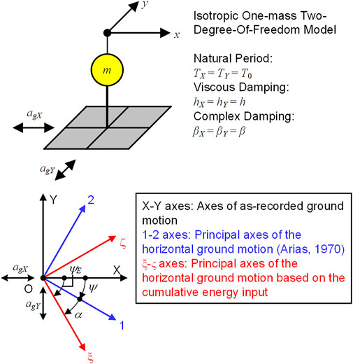
FIGURE 1. Definition of the principal axes of the horizontal ground motion.

In Eq. 1, the coefficients $c_{X,n}$ and $c_{Y,n}$ are the $n$th complex Fourier coefficients of the X- and Y-directions, respectively, and ${\omega }_n$ is the circular frequency of the $n$th harmonic. It is assumed that both $c_{X,0}$ and $c_{Y,0}$ are zero. The response velocity vector of the model is

$\mathbf{v}\left(t\right)=\left\{\begin{array}{c}{v}_X\left(t\right)\\ v_Y\left(t\right)\end{array}\right\}=\frac{d}{dt}\left\{\begin{array}{c}x\left(t\right)\\ y\left(t\right)\end{array}\right\}=-{\displaystyle \sum }_{n=-N}^N\left\{\begin{array}{c}{c}_{X,n}\\ c_{Y,n}\end{array}\right\}{H}_{CVV}\left(i{\omega }_n\right)\exp \left(i{\omega }_{n}t\right)(3)$

where

$H_{CVV}\left(i{\omega }_n\right)=i{\omega }_n{H}_{CVD}\left(i{\omega }_n\right)(4)$

$H_{CVD}\left(i{\omega }_n\right)=\frac{1}{{\omega }_0^2-{\omega }_n^2+2{\omega }_0\left\{h{\omega }_n+\beta {\omega }_0\mathrm{s}\mathrm{g}\mathrm{n}\left({\omega }_n\right)\right\}i}(5)$

$\mathrm{s}\mathrm{g}\mathrm{n}\left({\omega }_n\right)=\{\begin{array}{cc}1& :{\omega }_n>1\\ -1& :{\omega }_n<1\end{array}(6)$

In Eqs 3–6, $H_{CVV}\left(i{\omega }_n\right)$ and $H_{CVD}\left(i{\omega }_n\right)$ are the velocity and displacement transfer functions, respectively, ${\omega }_0\left(=2\pi /T_0\right)$ is the natural circular frequency of the model, and $i\left(=\sqrt{-1}\right)$ is the imaginary unit. The total (cumulative) input energy resulting from bidirectional ground motion, $E_I$, is defined as

$E_I=-m\underset{0}{\overset{t_d}{{\displaystyle \int }}}{\left\{\mathbf{v}\left(t\right)\right\}}^{\mathbf{T}}{\mathbf{a}}_{\mathbf{g}}\left(t\right)dt(7)$

The momentary input energy ($\Delta E_{BI}$) is defined as the energy input during a half cycle of the structural response (from $t$ to $t+\Delta t$):

$\Delta E_{BI}=-m\underset{t}{\overset{t+\Delta t}{{\displaystyle \int }}}{\left\{\mathbf{v}\left(t\right)\right\}}^{\mathbf{T}}{\mathbf{a}}_{\mathbf{g}}\left(t\right)dt(8)$

In Eq. 8, $\Delta t$ is the duration of a half cycle of the structural response. The maximum momentary input energy for bidirectional excitation ($\Delta E_{BI,\max }$) is defined as the maximum value of $\Delta E_{BI}$ over the course of a seismic event (Fujii and Murakami, 2020; Fujii 2021).

It is convenient to define the equivalent velocities of the total input energy ($V_I$) and the maximum momentary input energy ($V_{\Delta E}$) as

$V_I=\sqrt{2E_I/m},V_{\Delta E}=\sqrt{2\Delta E_{BI,\max }/m}(9)$

Next, we consider the cumulative energy input in each orthogonal ground motion component (the $\xi$- and $\varsigma$-axes shown in Figure 1) to the total input energy. The cumulative input energies in the $\xi$- and $\varsigma$-directions, $E_{I\xi }$ and $E_{I\varsigma }$, respectively, are defined as

$\{\begin{array}{l}{E}_{I\xi }=-m\underset{0}{\overset{t_d}{{\displaystyle \int }}}{v}_{\xi }\left(t\right)a_{g\xi }\left(t\right)dt\\ E_{I\zeta }=-m\underset{0}{\overset{t_d}{{\displaystyle \int }}}{v}_{\zeta }\left(t\right)a_{g\zeta }\left(t\right)dt\end{array}(10)$

where

$\left\{\begin{array}{l}{v}_{\xi }\left(t\right)\\ v_{\zeta }\left(t\right)\end{array}\right\}=\left[\begin{array}{cc}\cos {\psi }_E& -\sin {\psi }_E\\ \sin {\psi }_E& \cos {\psi }_E\end{array}\right]\left\{\begin{array}{l}{v}_X\left(t\right)\\ v_Y\left(t\right)\end{array}\right\}(11)$

and

$\left\{\begin{array}{l}{a}_{g\xi }\left(t\right)\\ a_{g\zeta }\left(t\right)\end{array}\right\}=\left[\begin{array}{cc}\cos {\psi }_E& -\sin {\psi }_E\\ \sin {\psi }_E& \cos {\psi }_E\end{array}\right]\left\{\begin{array}{l}{a}_{gX}\left(t\right)\\ a_{gY}\left(t\right)\end{array}\right\}(12)$

Using Eqs. 10, 11, 12 can be rewritten as

$\{\begin{array}{l}{E}_{I\xi }=E_{IXX}{\mathit{cos}}^2{\psi }_E-2E_{IXY}\mathit{sin}{\psi }_E\mathit{cos}{\psi }_E+E_{IYY}{\mathit{sin}}^2{\psi }_E\\ E_{I\zeta }=E_{IXX}{\mathit{sin}}^2{\psi }_E+2E_{IXY}\mathit{sin}{\psi }_E\mathit{cos}{\psi }_E+E_{IYY}{\mathit{cos}}^2{\psi }_E\end{array}(13)$

where

$\{\begin{array}{l}{E}_{IXX}=-m\underset{0}{\overset{t_d}{{\displaystyle \int }}}{v}_X\left(t\right)a_{gX}\left(t\right)dt\\ E_{IXY}=-\frac{1}{2}m\underset{0}{\overset{t_d}{{\displaystyle \int }}}\left\{v_X\left(t\right)a_{gY}\left(t\right)+v_Y\left(t\right)a_{gX}\left(t\right)\right\}dt\\ E_{IYY}=-m\underset{0}{\overset{t_d}{{\displaystyle \int }}}{v}_Y\left(t\right)a_{gY}\left(t\right)dt\end{array}(14)$

It is evident from Eq. 13 that the following relationship can be obtained:

$E_{I\xi }+E_{I\zeta }=E_{IXX}+E_{IYY}=E_I(15)$

Eq. 15 indicates that the sum of the cumulative input energies in each orthogonal direction is independent of the angle ${\psi }_E$ and equals the total input energy $E_I$.

Substituting Eqs 1, 3 into Eq. 7, the total input energy $E_I$ can be expressed as

$E_I=2m{t}_d{\displaystyle \sum }_{n=1}^N\mathrm{R}\mathrm{e}\left\{H_{CVV}\left(i{\omega }_n\right)\right\}\left\{{\left|c_{X,n}\right|}^2+{\left|c_{Y,n}\right|}^2\right\}(16)$

Similarly, $E_{IXX}$, $E_{IXY}$, and $E_{IYY}$ can be expressed as

$\{\begin{array}{l}{E}_{IXX}=2m{t}_d{\displaystyle \sum }_{n=1}^N\mathrm{R}\mathrm{e}\left\{H_{CVV}\left(i{\omega }_n\right)\right\}{\left|c_{X,n}\right|}^2\\ E_{IXY}=2m{t}_d{\displaystyle \sum }_{n=1}^N\mathrm{R}\mathrm{e}\left\{H_{CVV}\left(i{\omega }_n\right)\right\}\mathrm{R}\mathrm{e}\left(c_{X,n}\cdot c_{Y,-n}\right)\\ E_{IYY}=2m{t}_d{\displaystyle \sum }_{n=1}^N\mathrm{R}\mathrm{e}\left\{H_{CVV}\left(i{\omega }_n\right)\right\}{\left|c_{Y,n}\right|}^2\end{array}(17)$

Therefore, all cumulative energy quantities defined in Eqs. 7, 14 can be calculated from the Fourier complex coefficients of the ground motion sets.

2.2 Principal axis of the horizontal ground motion based on the cumulative energy input

Next, we consider the case in which the cumulative input energy $\xi$-axis reaches its maximum. In such a case, the angle ${\psi }_E$ can be determined from the following equation:

$\frac{d{E}_{I\xi }}{d{\psi }_E}=\frac{d}{d{\psi }_E}\left(E_{IXX}{\mathit{cos}}^2{\psi }_E-2E_{IXY}\mathit{sin}{\psi }_E\cos {\psi }_E+E_{IYY}{\mathit{sin}}^2{\psi }_E\right)=0(18)$

From Eq. 18, the angle ${\psi }_E$ can be easily obtained as

${\psi }_E=-\frac{1}{2}{\mathrm{Tan}}^{-1}\left(\frac{2E_{IXY}}{E_{IXX}-E_{IYY}}\right)(19)$

In this case, $E_{I\xi }$ and $E_{I\varsigma }$ can be calculated as

$\{\begin{array}{l}{E}_{I\xi }=\frac{E_{IXX}+E_{IYY}}{2}+\sqrt{{\left(\frac{E_{IXX}-E_{IYY}}{2}\right)}^2+E_{IXY}^2}\\ E_{I\zeta }=\frac{E_{IXX}+E_{IYY}}{2}-\sqrt{{\left(\frac{E_{IXX}-E_{IYY}}{2}\right)}^2+E_{IXY}^2}\end{array}(20)$

In the following discussion, the $\xi$- and $\varsigma$-axes denote the principal major and minor axes, respectively, of the horizontal ground motion based on the cumulative energy input. From Eqs 19, 20, Eq. 13 can be expressed in the form

$\left[\begin{array}{cc}{E}_{I\xi }& 0\\ 0& E_{I\zeta }\end{array}\right]=\left[\begin{array}{cc}\cos {\psi }_E& -\sin {\psi }_E\\ \sin {\psi }_E& \cos {\psi }_E\end{array}\right]\left[\begin{array}{cc}{E}_{IXX}& E_{IXY}\\ E_{IXY}& E_{IYY}\end{array}\right]\left[\begin{array}{cc}\cos {\psi }_E& \sin {\psi }_E\\ -\sin {\psi }_E& \cos {\psi }_E\end{array}\right](21)$

Eq. 21 indicates that the principal axes of the horizontal ground motion based on the cumulative energy input can be obtained from an eigenvalue analysis of the matrix ${\mathbf{E}}_{\mathbf{X}\mathbf{Y}}$ defined as

${\mathbf{E}}_{\mathbf{X}\mathbf{Y}}=\left[\begin{array}{cc}{E}_{IXX}& E_{IXY}\\ E_{IXY}& E_{IYY}\end{array}\right](22)$

It is also convenient to define the equivalent velocities of the cumulative energies in the major ($\xi$) and minor ($\varsigma$) directions ($E_{I\xi }$ and $E_{I\varsigma }$), respectively, as

$V_{I\xi }=\sqrt{2E_{I\xi }/m},V_{I\varsigma }=\sqrt{2E_{I\varsigma }/m}(23)$

The ratio of the equivalent velocity of the cumulative energies in the $\xi$- and $\varsigma$-directions ($R_{EI}$) is defined as

$R_{EI}=V_{I\varsigma }/V_{I\xi }(24)$

The range of the ratio $R_{EI}$ is 0–1. If $R_{EI}$ is smaller than $1/\sqrt{2}$, the cumulative input energy in the minor direction ($E_{I\varsigma }$) is less than half of that in the major direction ($E_{I\xi }$).

2.3 Comparisons with the principal axis of ground motion proposed by Arias and the cumulative energy-based principal axis

According to work by Arias (Arias, 1970), the principal axis of the horizontal ground motion is defined as the eigenvector of the matrix ${\mathbf{I}}_{\mathbf{A}\mathbf{X}\mathbf{Y}}$:

${\mathbf{I}}_{\mathbf{A}\mathbf{X}\mathbf{Y}}=\left[\begin{array}{cc}{I}_{AXX}& I_{AXY}\\ I_{AXY}& I_{AYY}\end{array}\right](25)$

where

$\{\begin{array}{l}{I}_{AXX}=\frac{\pi }{2g}\underset{0}{\overset{t_d}{{\displaystyle \int }}}{\left\{a_{gX}\left(t\right)\right\}}^{2}dt\\ I_{AXY}=\frac{\pi }{2g}\underset{0}{\overset{t_d}{{\displaystyle \int }}}\left\{a_{gX}\left(t\right)\right\}\left\{a_{gY}\left(t\right)\right\}dt\\ I_{AYY}=\frac{\pi }{2g}\underset{0}{\overset{t_d}{{\displaystyle \int }}}{\left\{a_{gY}\left(t\right)\right\}}^{2}dt\end{array}(26)$

In Eq. 26, $g$ is the gravitational acceleration. Figure 1 shows the principal axes of the horizontal ground motion according to Arias (the 1- and 2-axes). The angle of the 1-axis with respect to the X-axis, $\psi$, can be obtained from

$\psi =-\frac{1}{2}{\mathrm{Tan}}^{-1}\left(\frac{2I_{AXY}}{I_{AXX}-I_{AYY}}\right)(27)$

The Arias intensities of the horizontal major and minor components, $I_{A1}$ and $I_{A2}$, respectively, can be calculated as

$\{\begin{array}{l}{I}_{A1}=\frac{I_{AXX}+I_{AYY}}{2}+\sqrt{{\left(\frac{I_{AXX}-I_{AYY}}{2}\right)}^2+I_{AXY}^2}\\ I_{A2}=\frac{I_{AXX}+I_{AYY}}{2}-\sqrt{{\left(\frac{I_{AXX}-I_{AYY}}{2}\right)}^2+I_{AXY}^2}\end{array}(28)$

The following discussion focuses on how the difference between $\psi$ and ${\psi }_E$ arises. By substituting Eq. 1 into Eq. 26, each component of the matrix ${\mathbf{I}}_{\mathbf{A}\mathbf{X}\mathbf{Y}}$ can be calculated such that

$\{\begin{array}{l}{I}_{AXX}=\frac{\pi t_d}{g}{\displaystyle \sum }_{n=1}^N{\left|c_{X,n}\right|}^2\\ I_{AXY}=\frac{\pi t_d}{g}{\displaystyle \sum }_{n=1}^N\mathrm{R}\mathrm{e}\left(c_{X,n}\cdot c_{Y,-n}\right)\\ I_{AYY}=\frac{\pi t_d}{g}{\displaystyle \sum }_{n=1}^N{\left|c_{Y,n}\right|}^2\end{array}(29)$

The angle $\psi$ can be obtained as

$\psi =-\frac{1}{2}{\mathrm{Tan}}^{-1}\left\{\frac{2{\displaystyle \sum }_{n=1}^N\mathrm{R}\mathrm{e}\left(c_{X,n}\cdot c_{Y,-n}\right)}{{\displaystyle \sum }_{n=1}^N\left({\left|c_{X,n}\right|}^2-{\left|c_{Y,n}\right|}^2\right)}\right\}(30)$

In addition, the angle ${\psi }_E$ can be obtained from Eqs 17, 19 such that

${\psi }_E=-\frac{1}{2}{\mathrm{Tan}}^{-1}\left[\frac{2{\displaystyle \sum }_{n=1}^N\mathrm{R}\mathrm{e}\left\{H_{CVV}\left(i{\omega }_n\right)\right\}\mathrm{R}\mathrm{e}\left(c_{X,n}\cdot c_{Y,-n}\right)}{{\displaystyle \sum }_{n=1}^N\mathrm{R}\mathrm{e}\left\{H_{CVV}\left(i{\omega }_n\right)\right\}\left({\left|c_{X,n}\right|}^2-{\left|c_{Y,n}\right|}^2\right)}\right].(31)$

Comparisons of Eqs. 30, 31 indicate that the difference between the two angles ${\psi }_E$ and $\psi$ is that the angle ${\psi }_E$ depends on the properties of the linear system (e.g., the natural circular frequency ${\omega }_0$, complex damping ratio $\beta$, and viscous damping ratio $h$) while the angle $\psi$ depends only on the Fourier complex coefficients $c_{X,n}$ and $c_{Y,n}$.

Even though the angles ${\psi }_E$ and $\psi$ are different, there are special cases in which ${\psi }_E$ equals $\psi$. One example of such a case is shown by Igarashi and Gigyu (Igarashi and Gigyu, 2015). They proposed a procedure to synthesize spectrum-matched bidirectional accelerograms with specified values of the elliptical component of the polarization applicable to seismic performance assessments. Following their work, consider the case in which the Fourier complex coefficient in the Y-direction satisfies the following condition:

$c_{Y,n}=-i\cdot \gamma c_{X,n},c_{Y,-n}=i\cdot \gamma c_{X,-n}(32)$

Here, $\gamma$ (0 ≤ $\gamma$ ≤ 1) is the coefficient. From Eq. 32, the following terms can be calculated:

$\mathrm{R}\mathrm{e}\left(c_{X,n}\cdot c_{Y,-n}\right)=\mathrm{R}\mathrm{e}\left(i\gamma {\left|c_{X,n}\right|}^2\right)=0(33)$

Consider the case in which $\gamma$ is smaller than one. The angle $\psi$ can be easily calculated as

$\psi =-\frac{1}{2}{\mathrm{Tan}}^{-1}\left\{\frac{2{\displaystyle \sum }_{n=1}^N\mathrm{R}\mathrm{e}\left(i\gamma {\left|c_{X,n}\right|}^2\right)}{\left(1-{\gamma }^2\right){\displaystyle \sum }_{n=1}^N{\left|c_{X,n}\right|}^2}\right\}=-\frac{1}{2}{\mathrm{Tan}}^{-1}0=0(34)$

Similarly, the angle ${\psi }_E$ becomes zero when Eq. 32 is satisfied. In such a case, the principal axis of the horizontal ground motion defined in terms of the cumulative energy input ($\xi$-axis) coincides with the principal axis defined by Arias (1-axis). In this case, the ratio $R_{EI}$ is independent of the natural period of the linear system and equals $\gamma$.

In the following discussions, the difference angle between the $\xi$- and 1-axes, $\alpha$ shown in Figure 1, is defined as

$\alpha ={\psi }_E-\psi (35)$

As discussed above, the angle $\alpha$ depends on the properties of the linear system.

3 Building and ground motion data

3.1 Building data

The building model analyzed in this study is a base-isolated building model (Model-Tf44) that was used in a previous study (Fujii and Masuda, 2021). Figure 2 shows a simplified structural plan and the elevation of the main building of the former Uto City Hall (Fujii, 2019). The layout of the isolators and dampers in the isolation layer below level 0 are shown in Figure 3. The isolation layer comprises NRBs, ESBs, and steel dampers. As shown in the figures, the steel dampers were placed at the perimeter frames to provide torsional resistance. The point G shown in this figure is the center of mass of the superstructure, point S₀ is the center of stiffness of the isolation layer calculated according to the initial stiffness of the isolators and dampers, while point S₁ is the center of stiffness of the isolation layer calculated according to the secant stiffness of the isolators and dampers considering their displacement of 0.30 m. The eccentricity indices (Building Center Japan, 2016) of this model, calculated according to initial stiffnesses in the X and Y directions, were $R_{eX}$ = 0.155 and $R_{eY}$ = 0.126, respectively, while those calculated according to the secant stiffnesses in the X and Y directions were $R_{eX}$ = 0.228 and $R_{eY}$ = 0.015, respectively.

FIGURE 2

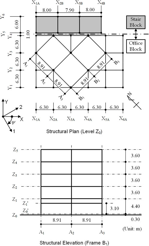
FIGURE 2. Simplified structural plan and elevation of the former Uto City Hall (Fujii, 2019).

FIGURE 3

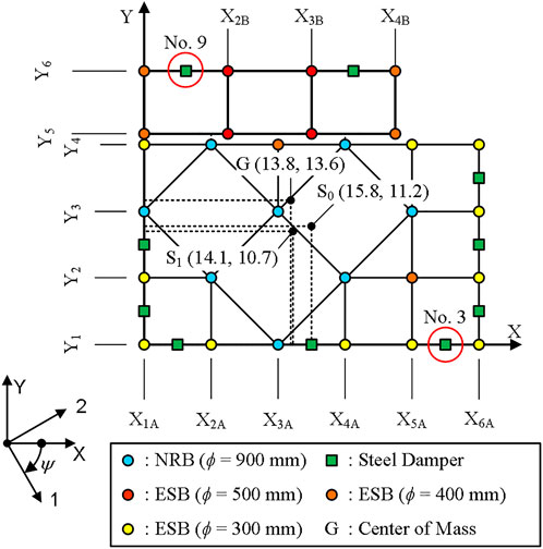
FIGURE 3. Layout of the isolators and dampers in the isolation layer (Fujii, 2021).

Figure 4 shows the structural modeling. The shear behavior of the NRBs was assumed to be linear elastic, while that of the ESBs and dampers was assumed to be normal bilinear. The vertical behavior of the NRBs and ESBs was assumed to be linear elastic. The shear behavior of the NRBs, ESBs, and steel dampers was modeled using a multi-shear spring model (Wada and Hirose, 1989). As in the previous study, the foundation compliance and kinematic soil-structure interaction were not considered for the simplicity of the analysis. Details concerning the original building and retrofitted building model can be found in previous studies (Fujii, 2019; Fujii and Masuda, 2021).

FIGURE 4

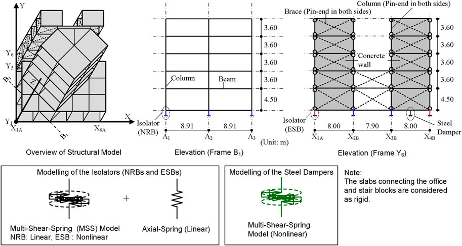
FIGURE 4. Structural modeling overview (Fujii, 2021).

3.2 Preliminary pushover analysis of a base-isolated building model

To understand the fundamental nonlinear behavior of the base-isolated building model, a pushover analysis was performed and then the nonlinear parameters were calculated. Here, the U-axis is the principal axis of the first modal response, while the V-axis is the axis perpendicular to the U-axis, following previous studies (Fujii, 2011; Fujii, 2015). In this study, the Displacement-Based Mode-Adaptive Pushover (DB-MAP) analysis presented in previous studies (Fujii, 2014; Fujii, 2019) was adopted.

Figure 5 shows the modal parameters calculated from the pushover analysis results. Here, $D_{1U}^{*}$ and $A_{1U}^{*}$ are the equivalent displacement and acceleration of the first modal response, respectively; $T_{1eff}$ is the effective period of the first modal response; and $V_{\Delta E\mu 1U}^{\ast }$ is the effective velocity of the hysteretic dissipated energy in a half cycle of the first modal response. In addition, ${\psi }_k$ is the angle of the principal axis of the kth modal response; $R_{\rho k}$ is the torsional index of the kth mode; and ${}_n{m}_k^{*}$ is the kth effective modal mass ratio with respect to the principal axis of the kth modal response. The equations for calculating the above modal parameters are shown in the Appendix.

FIGURE 5

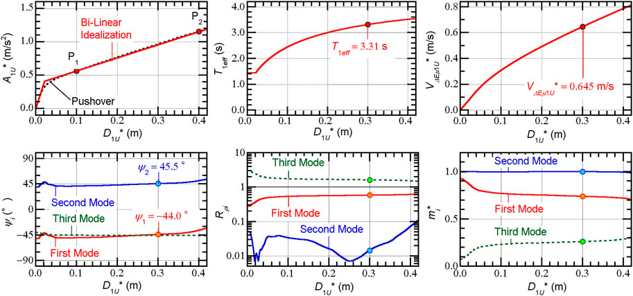
FIGURE 5. Modal parameters of the base-isolated model calculated from the pushover analysis results.

As shown in the upper left panel of Figure 5, the $A_{1U}^{\ast }$–$D_{1U}^{\ast }$ curve is idealized as bilinear to calculate the effective period ($T_{1eff}$) and the equivalent velocity of the hysteretic dissipated energy in a half cycle ($V_{\Delta E\mu 1U}^{\ast }$). In this study, the sets of ground motions are scaled such that the expected largest peak equivalent displacement of the first modal response (${D_{1U}}_{\max }^{*}$) considering all possible ASIs is 0.30 m as described later. Therefore, each parameter corresponding to $D_{1U}^{*}$ = 0.30 m is of interest. As shown in the upper middle panel of Figure 5, $T_{1eff}$ corresponding to $D_{1U}^{*}$ = 0.30 m is 3.31 s; meanwhile, $V_{\Delta E\mu 1U}^{\ast }$ corresponding to $D_{1U}^{\ast }$ = 0.30 m is 0.645 m/s, as shown in the upper right panel of Figure 5. The two parameters, $T_{1eff}$ and $V_{\Delta E\mu 1U}^{\ast }$, are used for the scaling of the ground motion sets later in this section.

The lower left panel of Figure 5 shows the change in the angle ${\psi }_k$ in terms of the equivalent displacement $D_{1U}^{*}$. The difference between the two angles ${\psi }_1$ and ${\psi }_2$ is close to 90°, while the angle ${\psi }_3$ is very close to ${\psi }_1$; the values of ${\psi }_1$ and ${\psi }_2$ corresponding to $D_{1U}^{*}$ = 0.30 m are −44.0° and 45.5°, respectively. The lower middle panel of Figure 5 shows the change in the torsional indices of the first three modes ($R_{\rho k}$). As shown here, $R_{\rho 1}$ is smaller than 1, $R_{\rho 2}$ is close to 0, and $R_{\rho 3}$ is larger than 1; the values of $R_{\rho 1}$, $R_{\rho 2}$, and $R_{\rho 3}$ corresponding to $D_{1U}^{*}$ = 0.30 m are 0.582, 0.014, and 1.615, respectively. The lower right panel of Figure 5 shows the change in the effective modal mass ratios of the first three modes ($m_k^{*}$). As shown here, $m_1^{*}$ is larger than 0.7, $m_2^{*}$ is close to 1, and $m_3^{*}$ is smaller than 0.3; the values of $m_1^{*}$, $m_2^{*}$, and $m_3^{*}$ corresponding to $D_{1U}^{*}$ = 0.30 m are 0.738, 0.999, and 0.261, respectively.

As discussed in previous studies (Fujii, 2016; Fujii, 2018), the first and second modes are predominantly translational ($R_{\rho 1},R_{\rho 2}<1$), while the third mode is predominantly torsional ($R_{\rho 3}>1$). Therefore, this base-isolated building model is classified as being torsionally stiff (TS) in both orthogonal directions.

Figure 6 shows the first mode shape corresponding to $D_{1U}^{*}$ = 0.30 m. As shown here, the superstructure behaves as a rigid body in the first mode. In addition, when the first modal response is predominant, the corner at which the largest horizontal displacement is expected is X_1AY₆. Note that, in a case in which there is unidirectional seismic input acting in an arbitrary direction, the largest first modal response occurs when the direction of the seismic input coincides with the principal axis of the first modal response (U-axis), according to shaking table tests of an elastic multi-story building model (Fujii and Ikeda, 2012). This finding has been supported in the nonlinear case examined in previous studies (e.g., Fujii, 2015; Fujii, 2016). Therefore, the angle ${\psi }_1$ (−44.0°) is an important structural parameter for discussing the influence of the ASI on the response of a structure.

FIGURE 6

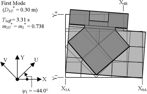
FIGURE 6. First mode shape corresponding to D_1U^* = 0.30 m.

3.3 Ground motion data

In this study, 10 horizontal ground motion sets from the NGA-West2 ground motion database of the Pacific Earthquake Engineering Research Center were used. Table 1 presents a list of the ground motion groups. Here, $M_W$ is the moment magnitude, $R_{rup}$ is the closest distance from the rupture plane, $T_p$ is the pulse period (Shahi et al., 2014), and $V_{S30}$ is the time-averaged shear-wave velocity in the top 30 m at the recording sites. These values were taken from the NGA-West2 ground motion database. As shown in Table 1, the range of $M_W$ is from 6.2 to 7.6, the range of $R_{rup}$ is from 0.89 km to 19.83 km, the range of $T_p$ is from 4.82 s to 10.40 s, and the range of $V_{S30}$ is from 206 m/s to 811 m/s.

TABLE 1

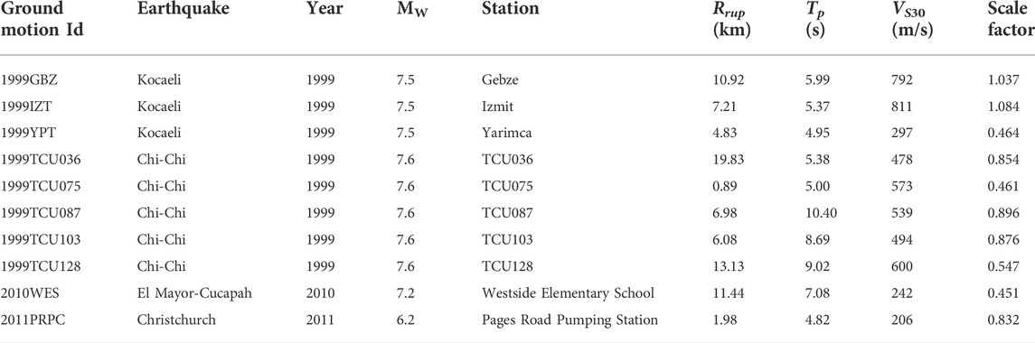
TABLE 1. List of the ground motion groups investigated in the present study.

Figure 7 shows the total input energy spectrum of the unscaled ground motion sets. For the calculation of the spectrum shown in Figure 7, the viscous damping ($h$) was set to 0.0 and the complex damping ($\beta$) was set to 0.10, based on a previous study (Fujii and Masuda, 2021). The variation of the angle $\alpha \left(T\right)$ is also shown. All ground motion sets used in this study satisfy the following condition:

$R_{EI}\left(T_{1eff}\right)=V_{I\varsigma }\left(T_{1eff}\right)/V_{I\xi }\left(T_{1eff}\right)<0.7(36)$

FIGURE 7

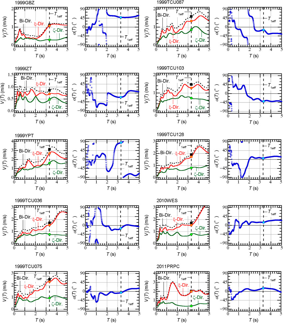
FIGURE 7. Total input energy spectra of the unscaled ground motion sets.

This condition was chosen to pick ground motion sets with significant directivity effects. As shown in Figure 7, the values of $V_{I\xi }\left(T\right)$ and $V_{I\varsigma }\left(T\right)$ are well separated around the effective period of the first modal response ($T_{1eff}$).

The angle $\alpha \left(T\right)$ shown here varies from zero; in other words, the principal axis of the horizontal ground motion based on the cumulative energy input ($\xi$-axis) is different from that proposed by Arias (1-axis). In addition, tendency of the angle $\alpha \left(T\right)$ depends on the ground motion set. The variation of $\alpha \left(T\right)$ is relatively stable near 2–4 s in some sets (e.g., 1999TCU075, 1999TCU128, 2010WES, and 2011PRPC), while notable variations are observed in other sets (e.g., 1999YPT and 1999TCU087).

3.4 Analysis method

The scaling method of the ground motion sets for the nonlinear time-history analysis is described as follows. According to a previous study (Fujii and Masuda, 2021), the largest peak equivalent displacement of the first modal response (${D_{1U}}_{\max }^{*}$) is predicted from the condition

$V_{\Delta E\mu 1U}^{\ast }\left(T_{1eff}\right)=V_{\Delta E}\left(T_{1eff}\right)(37)$

From Eq. 37, the scaling factor $\lambda$ can be calculated such that

$\lambda ={}_O{V}_{\Delta E}\left(T_{1eff},h,\beta \right)/V_{\Delta E\mu 1U}^{\ast }\left(T_{1eff}\right)(38)$

Here, ${}_O{V}_{\Delta E}\left(T_{1eff},h,\beta \right)$ is the equivalent velocity of the maximum momentary input energy of the unscaled ground motion sets calculated for a linear isotropic system (natural period $T=T_{1eff}$, viscous damping $h$, and complex damping $\beta$). The value of ${}_O{V}_{\Delta E}\left(T_{1eff},h,\beta \right)$ is calculated using a time-varying function of the momentary energy input formulated in previous studies (Fujii and Murakami, 2020; Fujii 2021).

Recall that the equivalent velocity of the hysteretic dissipated energy in a half cycle ($V_{\Delta E\mu 1U}^{\ast }$) is calculated from the pushover analysis result and that its value is 0.645 m/s as shown in Figure 5. The calculated scaling factor $\lambda$ for each ground motion set assuming $h$ = 0 and $\beta$ = 0.10 is given in Table 1. The maximum momentary input energy spectrum of the scaled ground motion sets is shown in Figure 8.

FIGURE 8

FIGURE 8. Maximum momentary input energy spectra of the scaled ground motion sets.

In this study, all unscaled ground motion sets are converted from the as-provided datasets to the horizontal major and minor components defined by Arias. In each nonlinear time-history analysis, the ASI ($\psi$) is defined as the angle between the 1-axis (the horizontal major axis of Arias) and the X-axis, as shown in Figure 2. The value of the ASI was set from −75° to 90° with an interval of 15°.

After the nonlinear time-history analysis is performed, the first and second modal responses are calculated using the method presented in a previous study (Fujii and Masuda, 2021). From this calculation, the time-history of the equivalent displacement of the first and second modal responses ($D_{1U}^{*}\left(t\right)$ and $D_{2V}^{*}\left(t\right)$) and the first mode vector corresponding to ${D_{1U}}_{\max }^{*}=\max \left\{\left|D_{1U}^{*}\left(t\right)\right|\right\}$ (${\Gamma }_{1U}{\mathbf{\phi }}_{\mathbf{1}}$) can be obtained. Then, the momentary input energy of the first modal response per unit mass is calculated such that

$\frac{\Delta E_{1U}^{\ast }}{M_{1U}^{*}}=-\underset{t}{\overset{t+\Delta t}{{\displaystyle \int }}}\left\{\frac{d}{dt}{D}_{1U}^{\ast }\left(t\right)\right\}{a}_{gU}\left(t\right)dt(39)$

Here, $a_{gU}\left(t\right)$ is the ground motion component of the U-axis (the principal axis of the first modal response corresponding to ${D_{1U}}_{\max }^{*}$ and calculated using ${\Gamma }_{1U}{\mathbf{\phi }}_{\mathbf{1}}$) and $\Delta t$ is the duration of a half cycle of the first modal response. The equivalent velocity of the maximum momentary input energy of the first modal response ($V_{\Delta E1U}^{\ast }$) is calculated such that

$V_{\Delta E1U}^{\ast }=\sqrt{2\Delta {E_{1U}}_{\max }^{*}/M_{1U}^{*}}(40)$

Here, $\Delta {E_{1U}}_{\max }^{*}/M_{1U}^{*}$ is the maximum momentary input energy of the first modal response per unit mass; it is also the maximum value of $\Delta E_{1U}^{*}/M_{1U}^{*}$ calculated using Eq. 39 over the course of the seismic event. Similarly, the cumulative input energy of the first modal response is calculated such that

$E_{I1U}^{\ast }=-M_{1U}^{\ast }\underset{0}{\overset{t_d}{{\displaystyle \int }}}\left\{\frac{d}{dt}{D}_{1U}^{\ast }\left(t\right)\right\}{a}_{gU}\left(t\right)dt(41)$

Here, $M_{1U}^{*}$ is the effective modal mass of the first mode and is assumed to be the value corresponding to ${D_{1U}}_{\max }^{*}$ for simplicity of calculation. Because the variation of $M_{1U}^{*}$ in terms of the equivalent displacement $D_{1U}^{*}$is relatively stable, as shown in Figure 5, it is likely that this approximation will not cause severe problems.

4 Analysis results and discussion

4.1 Peak response

In the following discussion, the peak response parameters focused on are (a) the maximum equivalent displacement of the first modal response (${D_{1U}}_{\max }^{*}$), (b) the equivalent velocity of the maximum momentary input energy of the first modal response ($V_{\Delta E1U}^{*}$), (c) the maximum equivalent displacement of the second modal response (${D_{2V}}_{\max }^{*}$), (d) the peak displacement of the frame Y₆ at level 5 (the roof), (e) the peak displacement of the frame X_1A at level 5, (f) the peak drift of column A₃B₃ at the second story, and (g) the peak resultant displacement of isolator X_1AY₆.

Figure 9 shows the relationship of the peak response and the ASI defined in terms of the principal axis of Arias ($\psi$). As shown in this figure, in general, the ASI that produces the largest response depends not only on the response quantities but also on the ground motion sets. For example, if we compare two cases, 1999YPT and 1999TCU075, the following observations can be made.

For 1999YPT, the largest ${D_{1U}}_{\max }^{*}$ and $V_{\Delta E1U}^{*}$ occur when the angle $\psi$ is 45°. Meanwhile, for 1999TCU075, the largest ${D_{1U}}_{\max }^{*}$ and $V_{\Delta E1U}^{\ast }$ occur when $\psi$ is −45°.

For 1999YPT, the largest ${D_{2V}}_{\max }^{*}$ occurs when $\psi$ is −60°. Meanwhile, for 1999TCU075, the largest ${D_{2V}}_{\max }^{*}$ occurs when $\psi$ is 45°.

According to the peak displacement of the frame Y₆ at level 5, the largest response occurs when $\psi$ is 75° for 1999YPT. Meanwhile, for 1999TCU075, the largest response occurs when $\psi$ is −15°.

According to the peak displacement of the frame X_1A at level 5, the largest response occurs when $\psi$ is 0° for 1999YPT. Meanwhile, for 1999TCU075, the largest response occurs when $\psi$ is −75°.

According to the peak drift of column A₃B₃ at the second story, the largest response occurs when $\psi$ is −15° for 1999YPT. Meanwhile, for 1999TCU075, the largest response occurs when $\psi$ is 90°.

According to the peak resultant displacement of isolator X_1AY₆, the largest response occurs when $\psi$ is 45° for 1999YPT. Meanwhile, for 1999TCU075, the largest response occurs when $\psi$ is −45°.

FIGURE 9

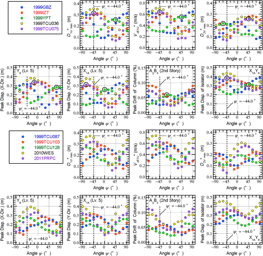
FIGURE 9. Relationship between the peak response and the angle of seismic incidence (ASI) defined in terms of the principal axis of Arias. Note that the plot at −90° is added to consider the symmetricity: the plots at −90° and 90° are the same. The black circled plots indicate the largest responses for the 1999YPT and 1999TCU075 cases.

Next, the relationship between the peak response and the ASI defined in terms of the principal axis based on the cumulative energy input (${\psi }_E$) is shown in Figure 10. In this figure, the angle ${\psi }_E$ is calculated such that

${\psi }_E=\alpha \left(T_{1eff}\right)+\psi (42)$

FIGURE 10

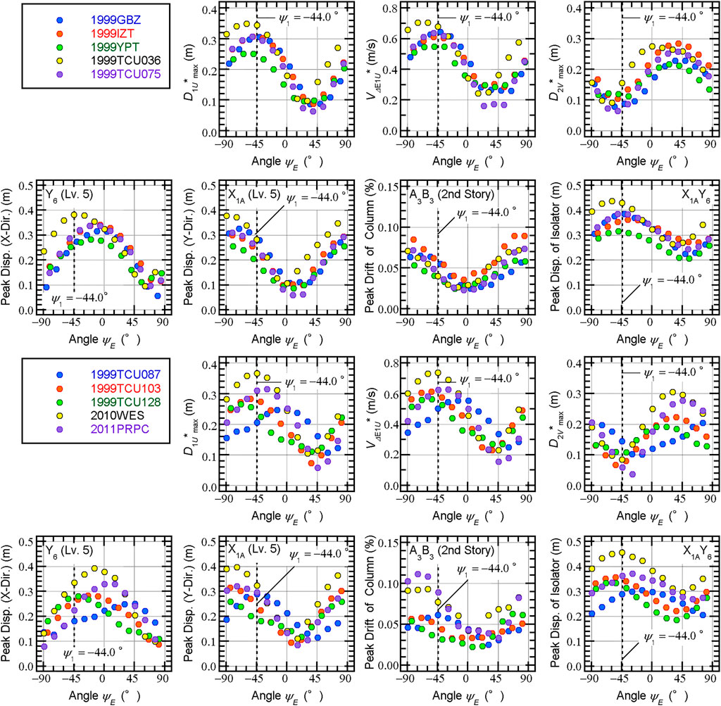
FIGURE 10. Relationship between the peak response and the ASI defined in terms of the principal axis based on the cumulative energy input.

As shown Figure 10, the angles ${\psi }_E$ that produce the largest response parameters are much closer in each ground motion set than those shown in Figure 9. The largest ${D_{1U}}_{\max }^{*}$ and $V_{\Delta E1U}^{\ast }$ occur when the angle ${\psi }_E$ is close to −45° in most cases. Meanwhile, the largest ${D_{2V}}_{\max }^{*}$ occurs when the angle ${\psi }_E$ is close to 45° in most cases. According to the local response quantities, the peak displacement of the frame Y₆ becomes larger when the angle ${\psi }_E$ is close to 0°, while that of the frame X_1A becomes larger when the angle ${\psi }_E$ is close to ±90°. The peak story drift at column A₃B₃ at the second story becomes larger when the angle ${\psi }_E$ is close to −75°, even though differences are observed for some ground motion sets. The peak resultant displacement of isolator X_1AY₆ becomes larger when the angle ${\psi }_E$ is close to −45°.

4.2 Cumulative response

Next, we examine the relationship between the cumulative response and the ASI defined in terms of the principal axis based on the cumulative energy input (${\psi }_E$). The response parameters focused on are (a) the total input energy ($E_I$), (b) the cumulative input energy of the first modal response ($E_{I1U}^{*}$), (c) the cumulative energy of damper No. 3, and (d) the cumulative energy of damper No. 9. The locations of dampers No. 3 and 9 are shown in Figure 3.

Figure 11 shows the relationship between the cumulative response and the angle ${\psi }_E$. This figure indicates that the variation of $E_I$ as a result of the different ASI values is small. Conversely, the variations of $E_{I1U}^{*}$ and the cumulative energy of the two dampers as a result of the different ASI values is significant. To see the changes in the three parameters as a result of different ASI values clearly, graphs in which these three parameters are normalized according to the total input energy are also shown. We see that the normalized cumulative input energy of the first modal response ($E_{I1U}^{\ast }/E_I$) becomes largest when ${\psi }_E$ is close to −45° in most cases. The normalized cumulative energy of damper No. 3 becomes largest when ${\psi }_E$ is close to 45°, while that of damper No. 9 becomes largest when ${\psi }_E$ is close to −45° in most cases.

FIGURE 11

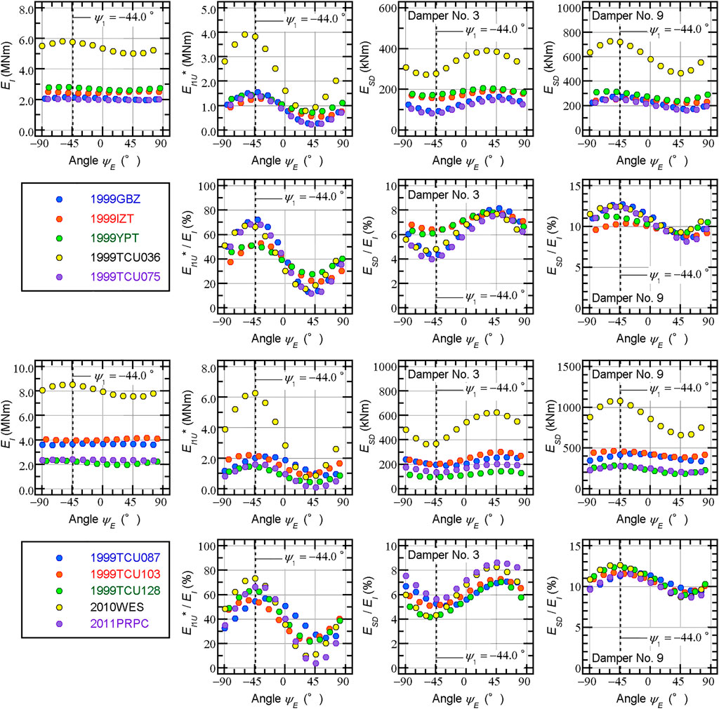
FIGURE 11. Relationship between the cumulative response and the ASI defined in terms of the principal axis based on the cumulative energy input.

4.3 Difference in the first modal response as a result of the incident angle

To understand the influence of the ASI on the first modal response, the hysteresis and time-history of the energy input were investigated. Figure 12 shows the hysteresis of the first modal response and the time-history of the energy input for two cases. The input ground motion set is 1999TCU075 and two ASIs are chosen: the first case has $\psi$ = −45° (${\psi }_E$ = −51.1°) and the second case has $\psi$ = 45° (${\psi }_E$ = 38.9°). The following observations can be made based on Figure 12.

When $\psi$ = −45° (${\psi }_E$ = −51.1°), the hysteresis of the first modal response is very regular. The final cumulative input energy of the first modal response ($E_{I1U}^{*}$) is 68.5% of the total input energy ($E_I$). In addition, the maximum momentary input energy of the first modal response ($\Delta {E_{1U}}_{\max }^{*}$) is 57.6% of $E_{I1U}^{*}$.

When $\psi$ = 45° (${\psi }_E$ = 38.9°), the hysteresis of the first modal response is irregular as a result of the nonlinear interactions of the other modes. The value of $E_{I1U}^{*}$ is only 11.9% of $E_I$. In addition, $\Delta {E_{1U}}_{\max }^{*}$ is 27.3% of $E_{I1U}^{*}$.

In both cases, the peak response occurs at the end of the half cycle of the first modal response when the maximum momentary input energy of the first modal response ($\Delta {E_{1U}}_{\max }^{*}$) occurs.

FIGURE 12

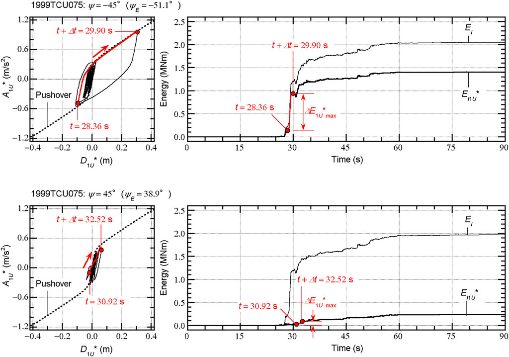
FIGURE 12. Hysteresis of the first modal response and the time-history of the energy input.

Next, the relationship between the first modal response and the local response is investigated. Figure 13 shows the displacement orbit of the four isolates at the corners for the $\psi$ = −45° and 45° cases. The input ground motion set is 1999TCU075, which is the same as that for the results shown in Figure 12. In Figure 13, the orbits obtained from the pushover (DB-MAP) analysis are also shown. The following observations can be made.

For the $\psi$ = −45° (${\psi }_E$ = −51.1°) case, the directions of the displacement of the isolators that occurred from 28.36 s to 29.90 s are close to the pushover analysis results, except for isolator X_6AY₁. The maximum resultant displacement of the four isolators occurs from 28.36 s to 29.90 s. The largest maximum resultant displacement is observed at isolator X_1AY₆.

For the $\psi$ = 45° (${\psi }_E$ = 38.9°) case, the directions of the displacements of the isolators that occurred from 30.92 s to 32.52 s are different from the pushover analysis results.

FIGURE 13

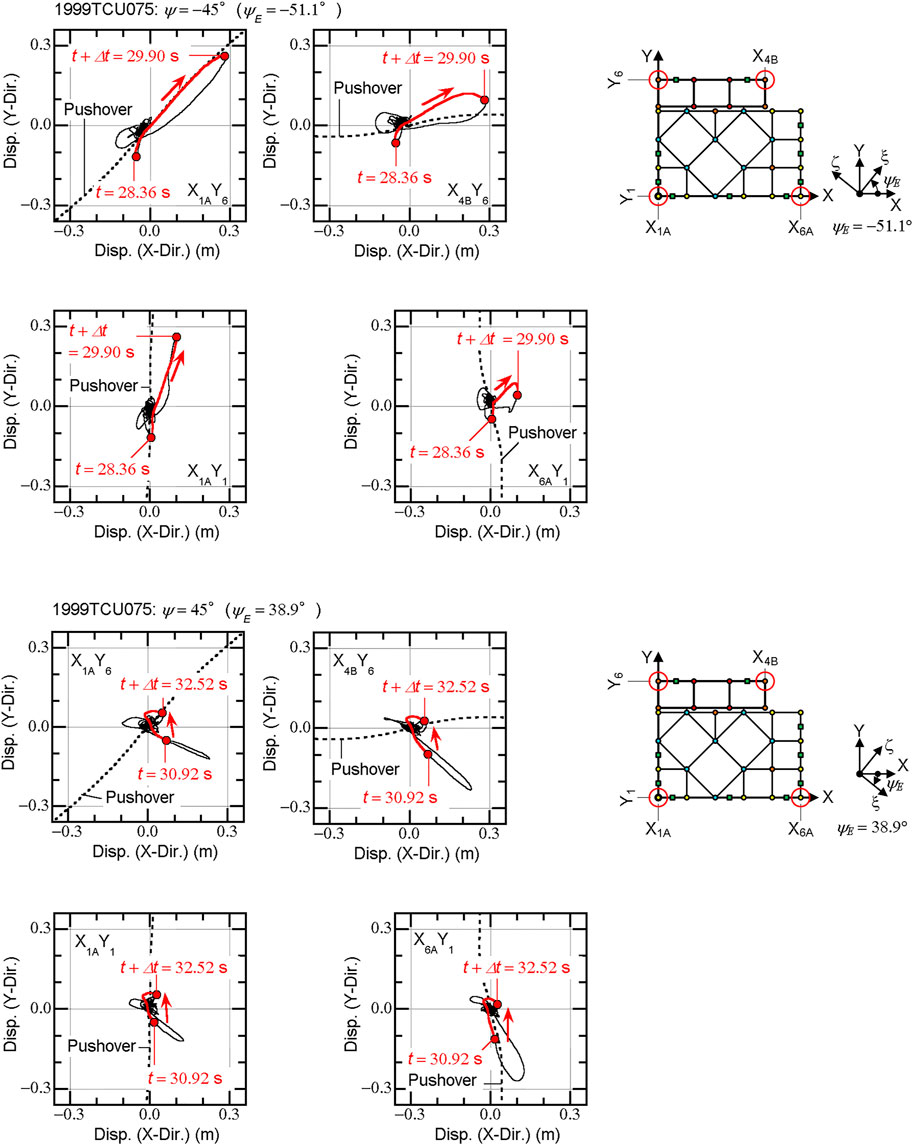
FIGURE 13. Displacement orbit of the four isolates at the corners.

Note that, in the $\psi$ = −45° (${\psi }_E$ = −51.1°) case, the maximum resultant displacement of the four isolators occurs during the half cycle when the maximum momentary input energy of the first modal response occurs. This observation is different in the $\psi$ = 45° (${\psi }_E$ = 38.9°) case.

Figure 14 shows the peak drift of the three columns A₁B₁, A₃B₁, and A₃B₃. The input ground motion set is 1999TCU075, which is the same as that for the results shown in Figures 12, 13. In this figure, the maximum and minimum values of all ASIs and the values of two ASIs ($\psi$ = −45° and $\psi$ = 45°, respectively) are shown. The following observations can be made.

The maximum peak drift of the three columns is less than 0.10%. Therefore, only minor damage is expected in the superstructure.

The peak drift of the two ASIs ($\psi$ = −45° and $\psi$ = 45°) are smaller than the maximum value. The critical ASI which produces the largest peak drift of the three columns are different from the ASI which produces the largest ${D_{1U}}_{\max }^{\ast }$, $V_{\Delta E1U}^{\ast }$, and $E_{I1U}^{\ast }$.

FIGURE 14

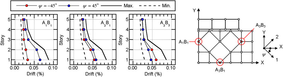
FIGURE 14. Peak drift of the three columns A₁B₁, A₃B₁, and A₃B₃ (1999TCU075).

The reason why the critical ASI which produces the largest peak drift of the three columns are different from the ASI which produces the largest ${D_{1U}}_{\max }^{*}$, $V_{\Delta E1U}^{*}$, and $E_{I1U}^{*}$ may be explained as follows. In the first mode, the superstructure behaves as a rigid body. Therefore, the contribution of the first modal response to the deformation of the superstructure is small. The deformation of the superstructure is significantly affected by the higher modal response.

4.4 Discussion

As previously noted, defining the angle of the critical axis of ground motion is essential to discuss the influence of the ASI on the nonlinear response of an irregular building structure. According to the results shown here, it is difficult to discuss this problem using an ASI based on the principal axis of ground motion proposed by Arias; as shown in Figure 9, the critical ASI of each response quantity differs notably depending on the ground motion set.

Conversely, the ASI based on the principal axis defined in terms of the cumulative energy input is more suitable to discuss this problem. As shown in Figures 10, 11, ${D_{1U}}_{\max }^{*}$, $V_{\Delta E1U}^{*}$, and $E_{I1U}^{*}$ are largest when the angle ${\psi }_E$ is close to the angle of the principal axis of the first modal response (${\psi }_1$). Conversely, ${D_{2V}}_{\max }^{*}$ is smallest when ${\psi }_E$ is close to ${\psi }_1$ in most cases. Therefore, there is no ASI value that produces both the largest ${D_{1U}}_{\max }^{*}$ and the largest ${D_{2V}}_{\max }^{*}$ simultaneously. This explains why the critical ASI differs depending on the response parameters: the critical ASI of each response parameter depends on the contributions of each modal response. For example, the peak resultant displacement of isolator X_1AY₆ becomes largest when ${\psi }_E$ is close to ${\psi }_1$ in most cases because the contribution of the first modal response to the response of isolator X_1AY₆ is predominant. Similarly, the cumulative strain energy of damper No. 3 becomes largest when ${\psi }_E$ is 45° because the contribution of the second modal response to the response of damper No. 3 is predominant while that of the first modal response is small. In addition, the critical ASI of the peak drift of three columns are different from that of the first modal response, as shown in Figure 14. This is because the deformation of the superstructure is significantly affected by the higher modal response.

Based on the discussions above, the author recommends to use the energy-based principal axis of horizontal ground motion as the reference axis of horizontal ground motion set for discussions concerning the influence of ASI on the response of an irregular base-isolated buildings. It enables to reduce the difference of the critical ASI depending on the ground motion set.

5 Conclusion

This study investigated the influence of the ASI values of long-period pulse-like seismic inputs on an irregular base-isolated building. The main conclusions and results are as follows.

Compared with the principal axis of ground motion proposed by Arias (Arias, 1970), the principal axis of ground motion defined in terms of the cumulative energy input is more suitable for discussions concerning the influence of the ASI on the response of an irregular base-isolated building.

The influence of the ASI of long-period pulse-like ground motions on the irregular base-isolated building studied here depends on the response parameters. The peak horizontal displacement of the top floor along the structural axes indicates that the peak displacement is notably affected by the ASI. Conversely, the variation in the total input energy as a result of different ASI values is very small.

The angles of the principal major axis of ground motion in terms of the cumulative energy input (${\psi }_E$) and the principal axis of the first modal response (${\psi }_1$) are key parameters to explain the influence of the ASI on the response of the irregular base-isolated building studied here. The peak equivalent displacement and the cumulative input energy of the first modal response are largest when the angle ${\psi }_E$ is close to ${\psi }_1$. In such a case, the contribution of the first modal response to the whole response becomes larger. For local response quantities in which the contribution of the first modal response is predominant, the critical ASI is close to ${\psi }_1$. Conversely, for local response quantities in which the contribution of the second modal response is predominant, the critical ASI differs by nearly 90°.

The principal axis of ground motion in terms of the cumulative energy input investigated here has the following advantages: (1) it can be directly calculated from the complex Fourier coefficients of the ground motion components without knowing the time-history of the ground motion; (2) the dependence of the dynamic properties of the structure are considered when calculating the principal axis; and (3) this is directly related to the cumulative response of the building. Note that the results shown in this study are, so far, valid only for an irregular base-isolated building model subjected to the 10 selected bidirectional ground motion sets. Therefore, apart from further verifications using additional building models and ground motion sets, the following questions remain.

The significance of the influence of the ASI on the nonlinear response of a base-isolated building depends on the degree of the irregularity of the building because, in most cases, isolators and dampers used in an isolation layer are designed to be isotropic in any horizontal direction. Therefore, the influence of the ASI on the nonlinear response of a base-isolated building may be increasingly pronounced as its structural irregularity increases (e.g., large eccentricity or insufficient torsional resistance in an isolation layer). How will the degree of irregularity of a base-isolated building affect the variation in the structural responses caused by changes in the ASI?

In this study, the ratio of the equivalent velocities of the cumulative energy input in the major and minor directions ($R_{EI}=V_{I\varsigma }/V_{I\xi }$) was considered to select horizontal ground motion sets with a notable directivity effect. It is expected that variations in the response parameters will be larger when $R_{EI}$ is close to 0, while variations will be smaller when $R_{EI}$ is close to 1. What is the relationship between the ratio $R_{EI}$ and the variation in the structural response parameters?

All the horizontal ground motion sets used in this study had long pulse periods as defined by Shahi and Baker (Shahi et al., 2014). In the case of ground motion sets with shorter pulse periods, the influence of the ASI on the nonlinear response of a base-isolated building will be different from the results found here. It is expected that the contributions of higher modal responses will be significant in such cases. Are the findings shown in this study still valid in such cases?

The principal axis of the horizontal ground motion set is defined in terms of the cumulative energy input over the course of a seismic event. Even though this definition is directly related to the cumulative response, it is uncertain as to whether this definition is suitable for the peak response. This definition of the principal axis may be useful for ground motion sets that are characterized by a small number of pulses in the same or similar directions. What if the direction of the predominant energy input changes during a seismic event? In such a case, the principal axis of the horizontal ground motion sets should be determined in terms of the energy input during a short time; this will allow the influence of the ASI on the peak response of the base-isolated building to be discussed rather than the principal axis determined in terms of the cumulative energy input over the course of the entire seismic input.

The above questions will be investigated in subsequent studies; however, they do not constitute a comprehensive list of all the issues remaining for further related studies.

Data availability statement

The raw data supporting the conclusions of this article will be made available by the authors, without undue reservation.

Author contributions

The author confirms being the sole contributor of this work and has approved it for publication.

Acknowledgments

The ground motions used in this study were obtained from the website of the Pacific Earthquake Engineering Research Center (https://ngawest2.berkeley.edu/, accessed on 16 July 2022). We thank Martha Evonuk, PhD, from Edanz (https://jp.edanz.com/ac), for editing a draft of this manuscript.

Conflict of interest

The author declares that the research was conducted in the absence of any commercial or financial relationships that could be construed as a potential conflict of interest.

Publisher’s note

All claims expressed in this article are solely those of the authors and do not necessarily represent those of their affiliated organizations, or those of the publisher, the editors and the reviewers. Any product that may be evaluated in this article, or claim that may be made by its manufacturer, is not guaranteed or endorsed by the publisher.

Supplementary material

The Supplementary Material for this article can be found online at: https://www.frontiersin.org/articles/10.3389/fbuil.2022.1034166/full#supplementary-material

References

Akiyama, H. (1985). Earthquake–resistant limit–state design for buildings. Tokyo: University of Tokyo Press.

Google Scholar

Architectural Institute of JAPAN (AIJ) (2016). Design recommendations for seismically isolated buildings. Tokyo: Architectural Institute of Japan.

Google Scholar

Arias, A. (1970). “A measure of earthquake intensity,” in Seismic design for nuclear power plants. Editor R. J. Hansen (Massachusetts, United States: The MIT Press), 438–483.

Google Scholar

Athanatopoulou, A. M. (2005). Critical orientation of three correlated seismic components. Eng. Struct. 27, 301–312. doi:10.1016/j.engstruct.2004.10.011

CrossRef Full Text | Google Scholar

Baker, J. W. (2007). Quantitative classification of near-fault ground motions using wavelet analysis. Bull. Seismol. Soc. Am. 97 (5), 1486–1501. doi:10.1785/0120060255

CrossRef Full Text | Google Scholar

Bray, J. D., and Rodriguez-Marek, A. (2004). Characterization of forward-directivity ground motions in the near-fault region. Soil Dyn. Earthq. Eng. 24, 815–828. doi:10.1016/j.soildyn.2004.05.001

CrossRef Full Text | Google Scholar

Bridgestone, C. (2017). Seismic isolation product line-up. Version 2017, Available at: https://www.bridgestone.com/products/diversified/antiseismic_rubber/pdf/catalog_201710.pdf (accessed on September 7, 2021).1

Google Scholar

Bugueño, I., Carvallo, J., and Vielma, J. C. (2022). Influence of directionality on the seismic response of typical RC buildings. Appl. Sci. (Basel). 12, 1534. doi:10.3390/app12031534

CrossRef Full Text | Google Scholar

Building Center of Japan (BCJ) (2016). The building standard law of Japan on CD-ROM. Tokyo: The Building Center of Japan.

Google Scholar

Cardone, D., and Gesualdi, G. (2014). Seismic rehabilitation of existing reinforced concrete buildings with seismic isolation: A case study. Earthq. Spectra 30 (4), 1619–1642. doi:10.1193/110612eqs323m

CrossRef Full Text | Google Scholar

Cavdar, E., and Ozdemir, G. (2022). Amplification in maximum isolator displacement of an LRB isolated building due to mass eccentricity. Bull. Earthq. Eng. 20, 607–631. doi:10.1007/s10518-021-01247-1

CrossRef Full Text | Google Scholar

Cavdar, E., and Ozdemir, G. (2020). Using maximum direction of a ground motion in a code-compliant analysis of seismically isolated structures. Structures 28, 2163–2173. doi:10.1016/j.istruc.2020.10.030

CrossRef Full Text | Google Scholar

Charleson, A., and Guisasola, A. (2017). Seismic isolation for architects. London, New York: Routledge.

Google Scholar

D’Amato, M., Gigliotti, R., and Laguardia, R. (2019). Seismic isolation for protecting historical buildings: A case study. Front. Built Environ. 5, 87. doi:10.3389/fbuil.2019.00087

CrossRef Full Text | Google Scholar

Faggella, M., Gigliotti, R., Mezzacapo, G., and Spacone, E. (2018). Graphic dynamic prediction of polarized earthquake incidence response for plan-irregular single story buildings. Bull. Earthq. Eng. 16, 4971–5001. doi:10.1007/s10518-018-0357-1

CrossRef Full Text | Google Scholar

Fontara, I. K. M., Kostinakis, K. G., and Athanatopoulou, A. M. (2012). “Some issues related to the inelastic response of buildings under Bi-directional excitation,” in Proceedings of the 15th World Conference on Earthquake Engineering, Lisbon, 24-28 September 2012.

Google Scholar

Fujii, K., and Masuda, T. (2021). Application of mode-adaptive bidirectional pushover analysis to an irregular reinforced concrete building retrofitted via base isolation. Appl. Sci. 11 (21), 9829. doi:10.3390/app11219829

CrossRef Full Text | Google Scholar

Fujii, K. (2015). “Application of the pushover-based procedure to predict the largest peak response of asymmetric buildings with buckling restrained braces,” in Proceedings of the 5th ECCOMAS Thematic Conference on Computational Methods in Structural Dynamics and Earthquake Engineering (COMPDYN), Crete Island, May 2015.

CrossRef Full Text | Google Scholar

Fujii, K. (2016). Assessment of pushover-based method to a building with bidirectional setback. Earthquakes Struct. 11 (3), 421–443. doi:10.12989/eas.2016.11.3.421

CrossRef Full Text | Google Scholar

Fujii, K. (2021). Bidirectional seismic energy input to an isotropic nonlinear one-mass two-degree-of-freedom system. Buildings 11, 143. doi:10.3390/buildings11040143

CrossRef Full Text | Google Scholar

Fujii, K. (2022). “Evaluating the effect of the various directions of seismic input on an irregular building: The former Uto city Hall,” in Seismic behaviour and design of irregular and complex civil structures IV. Editors R. Bento, M. De Stefano, D. Köber, and Z. Zembaty (Berlin, Germany: Springer), 201–213.

CrossRef Full Text | Google Scholar

Fujii, K., and Ikeda, T. (2012). “Shaking table test of irregular buildings under horizontal excitation act in arbitrary direction,” in Proceedings of the 15th World Conference on Earthquake Engineering, Lisbon, September 2012.

Google Scholar

Fujii, K., and Murakami, Y. (2020). “Bidirectional momentary energy input to a one-mass two-DOF system,” in Proceedings of the 17th World Conference on Earthquake Engineering, Sendai Japan, 27 Sep-02 Oct 2021.

Google Scholar

Fujii, K. (2011). Nonlinear static procedure for multi-story asymmetric frame buildings considering bi-directional excitation. J. Earthq. Eng. 15, 245–273. doi:10.1080/13632461003702902

CrossRef Full Text | Google Scholar

Fujii, K. (2014). Prediction of the largest peak nonlinear seismic response of asymmetric buildings under bi-directional excitation using pushover analyses. Bull. Earthq. Eng. 12, 909–938. doi:10.1007/s10518-013-9557-x

CrossRef Full Text | Google Scholar

Fujii, K. (2018). Prediction of the peak seismic response of asymmetric buildings under bidirectional horizontal ground motion using equivalent SDOF model. Jpn. Archit. Rev. 1 (1), 29–43. doi:10.1002/2475-8876.1007

CrossRef Full Text | Google Scholar

Fujii, K. (2019). Pushover-based seismic capacity evaluation of Uto city Hall damaged by the 2016 kumamoto earthquake. Buildings 9, 140. doi:10.3390/buildings9060140

CrossRef Full Text | Google Scholar

Güneş, N., and Ulucan, Z. Ç. (2019). Nonlinear dynamic response of a tall building to near-fault pulse-like ground motions. Bull. Earthq. Eng. 17, 2989–3013. doi:10.1007/s10518-019-00570-y

CrossRef Full Text | Google Scholar

Hall, J. F., Heaton, T. H., Halling, M. W., and Wald, D. J. (1995). Near-source ground motion and its effects on flexible buildings. Earthq. Spectra 11 (4), 569–605. doi:10.1193/1.1585828

CrossRef Full Text | Google Scholar

Hori, N., and Inoue, N. (2002). Damaging properties of ground motions and prediction of maximum response of structures based on momentary energy response. Earthq. Eng. Struct. Dyn. 31, 1657–1679. doi:10.1002/eqe.183

CrossRef Full Text | Google Scholar

Huang, Y. N., Whittaker, A. S., and Luco, N. (2008). Maximum spectral demands in the near-fault region. Earthq. Spectra 24 (1), 319–341. doi:10.1193/1.2830435

CrossRef Full Text | Google Scholar

Igarashi, A., and Gigyu, S. (2015). Synthesis of spectrum-compatible bi-directional seismic accelerograms with target elliptical component of polarization. Earthquake Resistant Engineering Structures X. WIT Trans. Built Environ. 152, 63–72.doi:10.2495/ERES150051

CrossRef Full Text | Google Scholar

Kalkan, E., and Kwong, N. S. (2013). Pros and cons of rotating ground motion records to fault-normal/parallel directions for response history analysis of buildings. J. Struct. Eng. (N. Y. N. Y). 140 (3), 1–14. doi:10.1061/(ASCE)ST.1943-541X.0000845

CrossRef Full Text | Google Scholar

Kalkan, E., and Reyes, J. C. (2015). Significance of rotating ground motions on behavior of symmetric- and asymmetric-plan structures: Part II. Multi-story structures. Earthq. Spectra 31 (3), 1613–1628. doi:10.1193/072012eqs242m

CrossRef Full Text | Google Scholar

Kashima, T., Koyama, S., Iiba, M., and Okawa, I. (2008). “Dynamic behaviour of a museum building retrofitted using base isolation system,” in Proceedings of the 14th World Conference on Earthquake Engineering, Beijing, China, October 12-17.

Google Scholar

Kostinakis, K. G., Athanatopoulou, A. M., and Avramidis, I. E. (2013). Evaluation of inelastic response of 3D single-story R/C frames under bi-directional excitation using different orientation schemes. Bull. Earthq. Eng. 11, 637–661. doi:10.1007/s10518-012-9392-5

CrossRef Full Text | Google Scholar

Lagaros, N. D. (2010). The impact of the earthquake incident angle on the seismic loss estimation. Eng. Struct. 32, 1577–1589. doi:10.1016/j.engstruct.2010.02.006

CrossRef Full Text | Google Scholar

Laguardia, R., Morrone, C., Faggella, M., and Gigliotti, R. (2019). A simplified method to predict torsional effects on asymmetric seismic isolated buildings under bi-directional earthquake components. Bull. Earthq. Eng. 17, 6331–6356. doi:10.1007/s10518-019-00686-1

CrossRef Full Text | Google Scholar

Lin, Y., He, X., and Igarashi, A. (2022). Influence of directionality of spectral-compatible Bi-directional ground motions on critical seismic performance assessment of base-isolation structures. Earthq. Eng. Struct. Dyn. 51, 1477–1500. doi:10.1002/eqe.3624

CrossRef Full Text | Google Scholar

Lopez, O. A., and Torres, R. (1997). The critical angle of seismic incidence and the maximum structural response. Earthq. Eng. Struct. Dyn. 26, 881–894. doi:10.1002/(sici)1096-9845(199709)26:9<881:aid-eqe674>3.0.co;2-r

CrossRef Full Text | Google Scholar

Magliulo, G., Maddaloni, G., and Petrone, C. (2014). Influence of earthquake direction on the seismic response of irregular plan RC frame buildings. Earthq. Eng. Eng. Vib. 13, 243–256. doi:10.1007/s11803-014-0227-z

CrossRef Full Text | Google Scholar

Penzien, J., and Watabe, M. (1975). Characteristics of 3-dimensional earthquake ground motions. Earthq. Eng. Struct. Dyn. 3, 365–373. doi:10.1002/eqe.4290030407

CrossRef Full Text | Google Scholar

Reyes, J. C., and Kalkan, E. (2015). Significance of rotating ground motions on behavior of symmetric- and asymmetric-plan structures: Part I. Single-story structures. Earthq. Spectra 31 (3), 1591–1612. doi:10.1193/072012eqs241m

CrossRef Full Text | Google Scholar

Rigato, A. B., and Medina, R. A. (2007). Influence of angle of incidence on seismic demands for inelastic single-storey structures subjected to bi-directional ground motions. Eng. Struct. 29, 2593–2601. doi:10.1016/j.engstruct.2007.01.008

CrossRef Full Text | Google Scholar

Ruggieri, S., and Uva, G. (2020). Accounting for the spatial variability of seismic motion in the pushover analysis of regular and irregular RC buildings in the new Italian building code. Buildings 10, 177. doi:10.3390/buildings10100177

CrossRef Full Text | Google Scholar

Seki, M., Miyazaki, M., Tsuneki, Y., and Kataoka, K. (2000). A Masonry school building retrofitted by base isolation technology, Proceedings of the 12th World Conference on Earthquake Engineering, January 2000, Auckland

Google Scholar

Shahi, S. K., Jack, W., and Baker, J. W. (2014). An efficient algorithm to identify strong-velocity pulses in multicomponent ground motions. Bull. Seismol. Soc. Am. 104 (5), 2456–2466. doi:10.1785/0120130191

CrossRef Full Text | Google Scholar

Skoulidou, D., and Romao, X. (2021). Are seismic losses affected by the angle of seismic incidence? Bull. Earthq. Eng. 19, 6271–6302. doi:10.1007/s10518-021-01121-0

CrossRef Full Text | Google Scholar

Skoulidou, D., and Romao, X. (2017). Critical orientation of earthquake loading for building performance assessment using lateral force analysis. Bull. Earthq. Eng. 15, 5217–5246. doi:10.1007/s10518-017-0176-9

CrossRef Full Text | Google Scholar

Skoulidou, D., and Romao, X. (2020). The significance of considering multiple angles of seismic incidence for estimating engineering demand parameters. Bull. Earthq. Eng. 18, 139–163. doi:10.1007/s10518-019-00724-y

CrossRef Full Text | Google Scholar

Somerville, P. G., Smith, N. F., Graves, R. W., and Abrahamson, N. A. (1997). Modification of empirical strong ground motion attenuation relations to include the amplitude and duration effects of rupture directivity. Seismol. Res. Lett. 68 (1), 199–222. doi:10.1785/gssrl.68.1.199

CrossRef Full Text | Google Scholar

Terenzi, G., Fuso, E., Sorace, S., and Costoli, I. (2020). Enhanced seismic retrofit of a reinforced concrete building of architectural interest. Buildings 10, 211. doi:10.3390/buildings10110211

CrossRef Full Text | Google Scholar

Wada, A., and Hirose, K. (1989). Elasto-plastic dynamic behaviors of the building frames subjected to bi-directional earthquake motions. J. Struct. Constr. Eng. 399, 37–47. in Japanese. doi:10.3130/aijsx.399.0_37

CrossRef Full Text | Google Scholar

Wilson, E. L., Suharwardy, I., and Habibulah, A. (1995). A clarification of the orthogonal effects in a three-dimensional seismic analysis. Earthq. Spectra 11 (4), 659–666. doi:10.1193/1.1585831

CrossRef Full Text | Google Scholar