 Yoshito Saotome1
 Kotaro Kojima
 Izuru Takewaki
- 1Department of Architecture and Architectural Engineering, Graduate School of Engineering, Kyoto University, Kyoto, Japan
- 2Faculty of Design and Architecture, Kyoto Institute of Technology, Kyoto, Japan
The collapse-limit input velocity level of the critical double impulse simulating the principal part of near-fault ground motions is derived for an elastic-plastic structure with viscous damping and P-delta effect. The structural system is modeled by a bilinear hysteretic SDOF system with negative post-yield stiffness reflecting the P-delta effect which plays a key role in the collapse behavior. Since the critical timing of the second impulse in the double impulse has been proven as the zero-restoring force timing after the first impulse for the elastic-plastic SDOF system with viscous damping, that property is used again in this paper. It is shown that the collapse-limit input level of the critical double impulse can be obtained as a function of the post-yield stiffness and the damping ratio by using the energy balance law and the quadratic-function approximation of the damping force-deformation relation. The applicability of the collapse-limit level to actual recorded ground motions is investigated through the time-history response analysis for the stable models and the collapse models under two actual earthquake ground motions.
Introduction
Dynamic instability induced by collapse is one of the most important and challenging problems in the field of earthquake-resistant design of building structures and infrastructures, and such phenomena have been investigated extensively from the theoretical and numerical viewpoints (Herrmann, 1965; Jennings and Husid, 1968; Sun et al., 1973; Tanabashi et al., 1973; Bertero et al., 1978; Takizawa and Jennings, 1980; Bernal, 1987, 1992, 1998; Nakajima et al., 1990; Ger et al., 1993; Challa and Hall, 1994; Hall, 1998; Hjelmstad and Williamson, 1998; Uetani and Tagawa, 1998; Araki and Hjelmstad, 2000; Sasani and Bertero, 2000; Williamson and Hjelmstad, 2001; Miranda and Akkar, 2003; Ibarra and Krawinkler, 2005, Sivaselvan et al., 2009; Adam and Jager, 2012; Khoshnoudian et al., 2014; Kojima and Takewaki, 2016a).
Jennings and Husid (1968) defined the statically stable limit for an elastic-plastic single-degree-of-freedom (SDOF) system with a rotational spring as the zero restoring moment in the plastic range. Sun et al. (1973) suggested a similar condition for a first-floor-braced structure and derived the stability limit of the SDOF system with a slip-type restoring force-deformation characteristic in free vibration with initial displacement and velocity. Ishida and Morisako (1985) derived numerically the stability boundary of an elastic-plastic structure subjected to the static gravity force and the horizontal harmonic force. Miranda and Akkar (2003) investigated the relation between the post-yield stiffness and the horizontal strength required to prevent dynamic instability through the response analysis of bilinear SDOF systems with the natural period 0.2–3.0 [sec] under 72 recorded ground motions. Khoshnoudian et al. (2014) examined the dynamic instability of a structure-soil system under 50 actual recorded pulse-like ground motions. These stability limits for SDOF systems have been applied to a multi-degree-of-freedom (MDOF) system (Takizawa and Jennings, 1980; Nakajima et al., 1990).
The dynamic stability has also been investigated for MDOF systems (Maier and Perego, 1992; Bernal, 1998; Uetani and Tagawa, 1998; Araki and Hjelmstad, 2000). Uetani and Tagawa (1998) proposed a method for predicting the deformation concentration under static and dynamic cyclic loading using the buckling mode of a simply supported beam with rotational springs representing the post-yield stiffness. Although a negative eigenvalue of a tangent stiffness matrix is well-known as a condition for static instability, dynamic instability cannot be determined only by the existence of the negative eigenvalue (Bernal, 1998). That is because the inertial force and the damping force can make the minimum eigenvalue positive. Bernal (1998) investigated the relation between the eigenvector and the sum of the inertial and damping forces in terms of dynamic instability and proposed a prediction method of dynamic instability by using the equivalent SDOF system. Araki and Hjelmstad (2000) proposed an additional condition for dynamic collapse based on the coincidence of the dynamic loading with the direction of motion considering an unloading process. Dynamic instability and collapse have been investigated for a frame model considering the material non-linearity and geometrical non-linearity (Ger et al., 1993; Challa and Hall, 1994; Hall, 1998; Sivaselvan et al., 2009).
However, previous studies provide only the stability or instability condition, e.g., “the zero-restoring-force point in the post-yield stiffness range” or “the negative eigenvalue by the tangent stiffness matrix.” On the other hand, Kojima and Takewaki (2016a) derived the collapse-limit input level of the double impulse for an undamped elastic-plastic SDOF system with the P-delta effect in the closed-form. The double impulse can represent the main part of the fling-step near-fault ground motion and the response to the double impulse can be expressed by only free vibration with the initial velocity. The collapse-limit level of the critical double impulse can be obtained by using the energy balance law where the kinetic energy by the initial velocity of mass is transformed into the sum of the elastic strain energy and the energy dissipated by the plastic deformation at the maximum displacement. Kojima and Takewaki (2016a) adopted the zero-restoring-force point in the post-yield stiffness range as the collapse point.
The phenomenon caused by the P-delta effect, which is represented by the negative second slope, may be related to the phenomenon of the rocking of a rigid block. Regarding the resonance and overturning phenomenon, some interesting researches have been conducted (Chatzis and Smyth, 2012; Makris and Vassiliou, 2013; Casapulla, 2015; Nabeshima et al., 2016; Casapulla and Maione, 2017).
In this paper, the collapse-limit input velocity level of the critical double impulse is derived approximately for an elastic-plastic structure with viscous damping and P-delta effect. The system is modeled by a damped bilinear hysteretic SDOF system with negative post-yield stiffness. The critical timing of the second impulse was proven as the zero-restoring force timing after the first impulse for the elastic-plastic SDOF system with viscous damping in the previous investigations (Kojima et al., 2017; Akehashi et al., 2018). By using the energy balance law and the quadratic-function approximation of the damping force-deformation relation (Kojima et al., 2017; Akehashi et al., 2018), it is shown that the collapse-limit input level of the critical double impulse can be obtained as a function of the post-yield stiffness and the damping ratio. It should be noted that, while the energy balance law for a damped bilinear hysteretic model with viscous damping was used in Akehashi et al. (2018), its applicability to the model with negative post-yield stiffness and viscous damping is still unclear. In addition, although the collapse-limit input velocity level of the critical double impulse was investigated for undamped models in the previous investigation (Kojima and Takewaki, 2016a), the collapse-limit input velocity level for damped models has never been made clear and the direct use of the previous method for undamped models is not possible. The investigation of the collapse-limit input velocity level for damped models is important in clarifying the significance of the role of damping, primarily provided by structural control technologies innovatively developed recently, to prevent the structural collapse.
The double impulse input and the model used in this study are explained in section Double Impulse and Damped Bilinear Hysteretic SDOF System With Negative Post-yield Stiffness. The collapse-limit input velocity level of the critical double impulse is derived for 4 collapse patterns in section Collapse Limit Input Level for Damped Bilinear Hysteretic SDOF System With Negative Post-yield Stiffness. Accuracy of the proposed approximate closed-form solution for the collapse-limit level is investigated through the time-history response analysis for stable and unstable models in section Accuracy Check for Approximate Collapse-Limit Input Velocity Level of Critical Double Impulse. The effect of the damping ratio on the collapse-limit input level is clarified in section Transition of Collapse-Limit Input Velocity Level With Respect to Damping Ratio. Applicability of the proposed solution of the collapse level to the one-cycle sinusoidal wave is investigated through the comparison of the proposed level of the double impulse and that of the one-cycle sinusoidal wave in section Applicability of the Proposed Collapse-Limit Input Level to the Corresponding One-Cycle Sinusoidal Wave. Further applicability of the proposed theory to actual near-fault ground motions is discussed in section Applicability of the Proposed Collapse-Limit Input Level to Actual Recorded Ground Motions. The conclusions are summarized in section Conclusions.
Double Impulse and Damped Bilinear Hysteretic SDOF System With Negative Post-yield Stiffness
A ground acceleration üg(t) is expressed in the form of the double impulse as shown in Figure 1A (Kojima and Takewaki, 2015, 2016a,b).
where V denotes the velocity provided by the double impulse (the input velocity level), t0 denotes the time interval between two impulses and δ(t) is the Dirac's delta function.
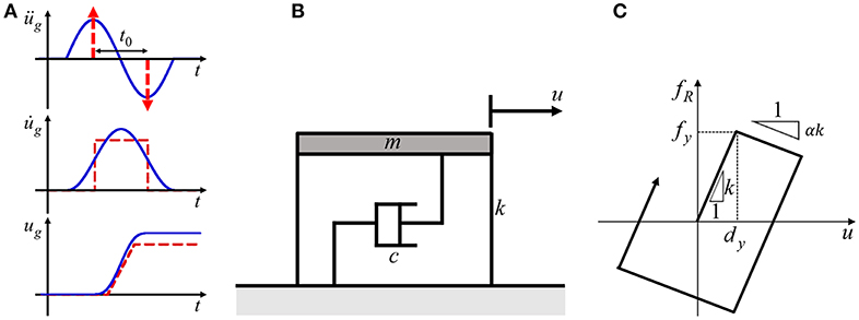
Figure 1. Input motion and damped bilinear hysteretic SDOF system, (A) Double impulse and one-cycle sinusoidal input as a principal component of near-fault ground motion, (B) Damped SDOF system with negative post-yield stiffness, (C) Bilinear hysteretic restoring-force characteristic with negative post-yield stiffness.
Consider a damped bilinear hysteretic SDOF system with negative post-yield stiffness as shown in Figure 1B. This SDOF system represents the elastic-perfectly plastic SDOF system under the consideration of stiffness reduction by the P-delta effect. m, c, and k denote the mass, damping coefficient and initial elastic stiffness of the SDOF system, respectively. , T1 = 2π/ω1 and are the undamped natural circular frequency, the undamped natural period and the damping ratio of this SDOF system, respectively. In this paper, the damping ratio is treated as constant regardless of yielding. u denotes the horizontal displacement of the mass relative to the ground as shown in Figure 1B, and the restoring force and damping force of the SDOF system are denoted by fR and fD, respectively. The yield deformation is given by dy and the yield force is by fy = kdy. The bilinear hysteretic restoring-force characteristic with the negative post-yield stiffness is shown in Figure 1C and the ratio of the post-yield stiffness to the initial elastic stiffness is denoted by α(< 0). Vy = ω1dy is the input velocity level of the single impulse at which the maximum deformation of the undamped SDOF system just attains the yield deformation dy and Vy is used to normalize the input velocity level V. In the determination of α, it is recommended to conduct the pushover analysis of the object frame under the P-delta effect. In the numerical examples in this paper, the results will be presented for various values of α.
Collapse Limit Input Level for Damped Bilinear Hysteretic SDOF System With Negative Post-yield Stiffness
The collapse-limit input velocity level of the double impulse is derived for the bilinear hysteretic SDOF system with the negative post-yield stiffness ratio α and the damping ratio h. It should be emphasized that, while the damping ratio h has never been included in the collapse-limit input velocity level in the previous investigation for the undamped model (Kojima and Takewaki, 2016a), it is included explicitly in the present paper for the damped model. Figure 2 shows the schematic diagrams of the restoring force-deformation relation and the damping force-deformation relation of the SDOF system under the critical double impulse. Figure 2A shows the stable case and Figure 2B indicates the collapse case. umax 1, up1, umax 2, up2 denote the maximum deformation and the plastic deformation after the first and second impulses, respectively. Note that umax 1, umax 2 are the absolute values. The critical timing of the second impulse is the zero-restoring force timing after the first impulse for the elastic-plastic SDOF system with viscous damping (Kojima et al., 2017; Akehashi et al., 2018). The mass velocity at the zero-restoring force timing (just before the second impulse) is denoted by vc.
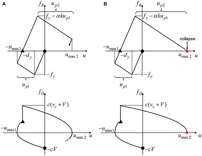
Figure 2. Restoring force-deformation relation and damping force-deformation relation of damped bilinear hysteretic SDOF system with negative post-yield stiffness under critical double impulse, (A) Stable state, (B) Collapse state (•: First impulse, ▴: Second impulse).
The collapse limit is characterized by the zero-restoring force point in the negative post-yield stiffness range and four collapse patterns, where the maximum deformation under the critical double impulse just attains the collapse limit (stability limit), are assumed as shown later. The collapse-limit input velocity level of the critical double impulse is derived via the energy balance law and the quadratic-function approximation of the damping force-deformation relation and the normalized collapse-limit input level V/Vy is obtained as a function of the post-yield stiffness ratio α and the damping ratio h. The energy balance law means that the kinetic energy just after the first or second impulse is transformed into the sum of the elastic strain energy, the energy dissipated by the plastic deformation and the energy dissipated by the viscous damping.
The four collapse patterns can be categorized as follows.
Collapse Pattern 1: Collapse limit after the second impulse without plastic deformation after the first impulse
Collapse Pattern 2: Collapse limit after the second impulse with plastic deformation after the first impulse
Collapse Pattern 3: Collapse limit after the second impulse with closed-loop in the restoring force-deformation relation
Collapse Pattern 4: Collapse limit after the first impulse.
The collapse-limit input levels in Collapse Patterns 1–4 are derived in the following sections.
Collapse Pattern 1: Collapse Limit After the Second Impulse Without Plastic Deformation After the First Impulse
The first collapse pattern represents the pattern where the SDOF system just attains the zero restoring force in the second stiffness range after the second impulse without plastic deformation after the first impulse. Figure 3 shows the restoring force-deformation relation and the damping force-deformation relation in Collapse Pattern 1. The input velocity level V/Vy in Collapse Pattern 1 has to satisfy the following equation since the plastic deformation is allowed only after the second impulse (Akehashi et al., 2018).
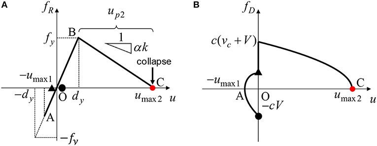
Figure 3. Elastic-plastic response corresponding to Collapse Pattern 1, (A) Restoring force-deformation relation, (B) Approximate damping force-deformation relation (Collapse limit after the second impulse without plastic deformation after the first impulse).
The left-hand side of the above inequality indicates the input velocity level at which the damped bilinear hysteretic SDOF system just attains the yield deformation after the second impulse and the right-hand side corresponds to the input velocity level at which the SDOF system just attains the yield deformation after the first impulse.
From Figure 3, the energy balance law after the second impulse can be described as
The left-hand side of Equation (3) indicates the kinetic energy for the velocity (vc + V) just after the second impulse and the right-hand side of Equation (3) expresses the sum of the elastic strain energy corresponding to the yield deformation, the energy dissipated by the plastic deformation and the energy dissipated by viscous damping. The energy dissipated by viscous damping is approximately obtained by using the quadratic-function approximation for the damping force-deformation relation (Kojima et al., 2017; Akehashi et al., 2018). Equation (3) can be transformed into the following equation by using umax 2 = dy + up2.
It can also be understood from Figure 3 that, when the maximum deformation after the second impulse just attains the collapse limit (the zero restoring force), the plastic deformation up2 after the second impulse can be obtained from fy + αkup2 = 0. Then up2 can be derived as
Let vc denote the velocity of the state when the restoring force becomes zero in the unloading process. It can be obtained by solving the equation of motion in the unloading process (point A to point O in Figure 3) (Kojima et al., 2017; Akehashi et al., 2018).
By substituting Equations (5) and (6) into Equation (4), the following equation is obtained.
From Equation (7), the input velocity level V/Vy of the critical double impulse in Collapse Pattern 1 can be derived by characterizing that the SDOF system just attains the zero-restoring force in the post-yield stiffness range after the second impulse without the plastic deformation after the first impulse.
where Inequality (2) should be satisfied.
Collapse Pattern 2: Collapse Limit After the Second Impulse With Plastic Deformation After the First Impulse
The second collapse pattern expresses the pattern such that the SDOF system just attains the collapse limit (the zero-restoring force in the second stiffness range) after the second impulse with the plastic deformation after the first impulse. Figure 4 shows the restoring force-deformation relation and the damping force-deformation relation in Collapse Pattern 2. The input velocity level V/Vy in Collapse Pattern 2 has to satisfy the following equation since the plastic deformation is allowed even after the first impulse (Akehashi et al., 2018).
From Figure 4, the energy balance law after the second impulse can be described as
The left-hand side of Equation (10) represents the kinetic energy for the velocity (vc + V) just after the second impulse. The right-hand side of Equation (10) expresses the sum of the elastic strain energy, the energy dissipated by the plastic deformation and the work done by the damping force. The work done by the damping force can be obtained by the quadratic-function approximation for the damping force-deformation relation (Akehashi et al., 2018).
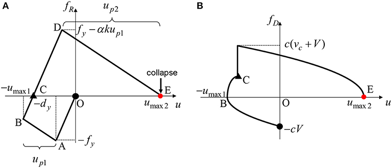
Figure 4. Elastic-plastic response corresponding to Collapse Pattern 2, (A) Restoring force-deformation relation, (B) Approximate damping force-deformation relation (Collapse limit after second impulse with plastic deformation after first impulse).
It can also be understood from Figure 4 that, since the maximum deformation after the second impulse just attains the collapse limit (the zero restoring force) with the plastic deformation after the first impulse, the plastic deformation up2 after the second impulse is calculated from fy − αkup1 + αkup2 = 0. Then, up2 can be expressed by
By substituting Equation (11) into Equation (10) and dividing both side of the resulting equation by (), the following equation can be obtained.
With the notation 1 − αup1/dy = A, Equation (12) can be transformed into the following equation.
From Equation (13), the normalized velocity (vc + V)/Vy just after the second impulse can be derived by
where .
Note that vc denotes the velocity of the state when the restoring force becomes zero in the unloading process. It can be obtained by solving the equation of motion in the unloading process (point B to point C in Figure 4) (Akehashi et al., 2018).
With the notation and by substituting Equation (15) into Equation (14), the following equation can be obtained.
The plastic deformation up1/dy after the first impulse can be obtained from the following energy balance law after the first impulse (Akehashi et al., 2018).
From Equation (17), up1/dy can be obtained by
where . By substituting Equation (18) and 1 − αup1/dy = A into Equation (16), the following equation can be obtained.
From the definition of D, Equation (19) provides the following quadratic equation for (V/Vy).
where .
From Equation (20), the input velocity level V/Vy of the critical double impulse in Collapse Pattern 2 can be derived by characterizing that the SDOF system just attains the zero-restoring force in the post-yield stiffness range after the second impulse with the plastic deformation after the first impulse.
where Inequality (9) should be satisfied.
Collapse Pattern 3: Collapse Limit After Second Impulse With Closed-Loop in Restoring Force-Deformation Relation
The third collapse pattern is the pattern such that the SDOF system just attains the collapse limit after the second impulse with a closed loop in the restoring force-deformation relation. In this collapse pattern, the SDOF system yields even after the first impulse [the input velocity level V/Vy must satisfy Inequality (9) as with Collapse Pattern 2] and the direction of the collapse limit is same as the maximum deformation after the first impulse. Figure 5 shows the restoring force-deformation relation and the damping force-deformation relation in Collapse Pattern 3.
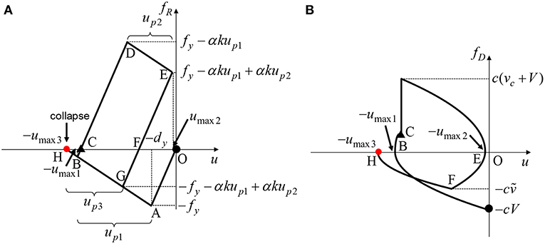
Figure 5. Elastic-plastic response corresponding to Collapse Pattern 3, (A) Restoring force-deformation relation, (B) Approximate damping force-deformation relation (Collapse limit after second impulse with closed-loop in restoring force-deformation relation and plastic deformation after first impulse).
The following equation can be obtained from the energy balance law between Point E and Point H in Figure 5.
Point E indicates the starting point in the unloading process after experiencing the maximum deformation after the second impulse and Point H is the point at which the maximum deformation after experiencing the closed loop after the second impulse attains the collapse limit in the same direction as the maximum deformation after the first impulse. Let ṽ denote the maximum velocity in the unloading process after the second impulse. Note that ṽ is the absolute value. The left-hand side of Equation (22) expresses the elastic strain energy at Point E and the right-hand side indicates the sum of the elastic strain energy, the energy dissipated by the plastic deformation and the work done by the damping force. The work done by the damping force between Point E and Point H is obtained by the quadratic-function approximation for the damping force-deformation relation (Akehashi et al., 2018).
By substituting ṽ into Equation (22) and arranging the resulting equation, a quartic equation of V/Vy can be derived. The detailed analysis of ṽ and the quartic equation is presented in Appendix. Then, the input velocity level V/Vy in Collapse Pattern 3 can be computed by solving the quartic equation. The collapse-limit level has to be a real number and satisfy Inequality (9).
Collapse Pattern 4: Collapse Limit After First Impulse
The fourth collapse pattern expresses the pattern in which the SDOF system just attains the collapse limit (the zero-restoring force in the post-yield stiffness range) after the first impulse. In Collapse Pattern 4, the input velocity level V/Vy must satisfy Inequality (9) as in Collapse Patterns 2 and 3.
From Figure 6, the following energy balance law between the point at the first impulse (Point O in Figure 6) and the point at the maximum deformation after the first impulse (Point B in Figure 6).
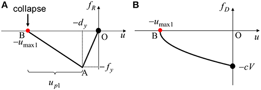
Figure 6. Elastic-plastic response corresponding to Collapse Pattern 4, (A) Restoring force-deformation relation, (B) Approximate damping force-deformation relation (Collapse limit after first impulse).
The left-hand side of Equation (23) indicates the kinetic energy calculated for the velocity V just after the first impulse. The right-hand side means the sum of the elastic strain energy corresponding to the yield deformation, the energy dissipated by the plastic deformation and the energy dissipated by the damping force. The energy dissipated by the damping force is obtained by the quadratic-function approximation for the damping force-deformation relation (Akehashi et al., 2018).
It can also be understood from Figure 6 that, when the maximum deformation after the first impulse just attains the zero-restoring-force point in the second stiffness range, the plastic deformation up1 after the first impulse can be obtained from
By substituting up1 = −dy/α derived from Equation (24) into Equation (23) and arranging the equation, the following equation can be derived.
By solving Equation (25), the input velocity level in Collapse Pattern 4 can be obtained as follows.
where Inequality (9) should be satisfied.
Accuracy Check for Approximate Collapse-Limit Input Velocity Level of Critical Double Impulse
The approximate collapse-limit input velocity levels of the critical double impulse in Collapse Patterns 1–4 were derived in section Collapse Limit Input Level for Damped Bilinear Hysteretic SDOF System With Negative Post-yield Stiffness. The collapse-limit level with respect to the negative post-yield stiffness ratio for damping ratio h = 0.10 is shown in Figure 7A with the schematic diagrams of the collapse patterns. It should be pointed out that the collapse-limit input velocity level corresponding to h = 0 was shown in Kojima and Takewaki (2016a). The shaded area in Figure 7A indicates the collapse region in the relation between the input level V/Vy and the post-yield stiffness ratio α. Case 1 in Figure 7A indicates the elastic case, Case 2 expresses the case with the plastic deformation only after the second impulse and Case 3 is the case with the plastic deformation even after the first impulse. Stability of the elastic-plastic system under the critical double impulse can be determined by the proposed solutions for various V/Vy, α, and h. The approximate input level for Collapse Pattern 4 becomes smaller than that for Collapse Pattern 3 in larger post-yield stiffness ratio (in the vicinity of α = 0). However, it should be kept in mind that this reversed phenomenon may result from the numerical error caused by the quadratic-function approximation of the damping force-deformation relation. This reversed phenomenon was not observed in the undamped model (Kojima and Takewaki, 2016a).
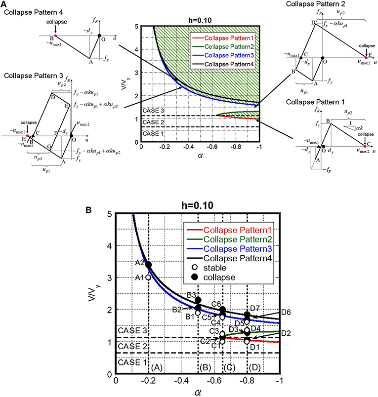
Figure 7. Collapse-limit input velocity level of critical double impulse with respect to post-yield stiffness ratio for specific damping ratio (h = 0.10), (A) Collapse-limit input level of critical double impulse and schematic diagram of Collapse Patterns 1–4, (B) Input velocity level and post-yield stiffness ratio for investigation (A1—D6).
In this section, the accuracy of the proposed collapse-limit level is investigated through the comparison with the time-history response analysis result. Figure 7B shows 18 points for models with damping ratio h = 0.10 to investigate the proposed collapse-limit level. The points indicate the set of input velocity levels of the double impulse velocity level V/Vy and the negative post-yield stiffness ratio α. These 18 points express the slightly larger or smaller than the approximate collapse-limit level with α = −0.20, −0.50, −0.65, −0.80. The restoring force-deformation relations of 18 points are shown in Figure 8. The blank circles indicate the stable cases and the solid circles express the collapse case evaluated by time-history response analysis. From Figure 8, the proposed method can evaluate stability or collapse in 18 points approximately, although the slightly dangerous level is provided in Collapse patterns 1 and 3 because of approximation accuracy.
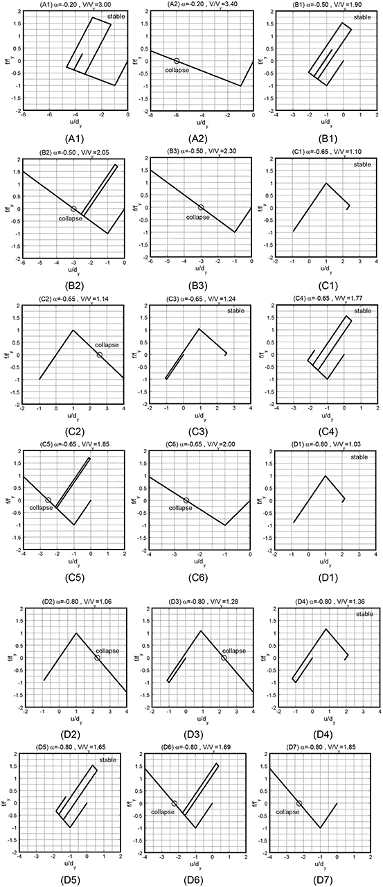
Figure 8. Restoring force-deformation relation of 18 stability or collapse cases (damping ratio h = 0.10).
In order to investigate the collapse-limit level in detail, the input velocity level of the critical double impulse at which the maximum deformation just attains the collapse limit is evaluated by the time-history response analysis. The elastic-plastic response to the critical double impulse can be evaluated by changing the time interval in a parametric manner in the time-history response analysis. Figure 9 shows the comparison of the collapse-limit level by the proposed theory and that by the time-history response analysis for h = 0.05, 0.10. The minimum collapse-limit level by the time-history response analysis is only plotted in Figure 9, although there is the stable region between Collapse Pattern 2 and Collapse Pattern 3 for the critical double impulse. The minimum collapse-limit level by the time-history response analysis corresponds to Collapse Pattern 1 in the smaller post-yield stiffness ratio. On the other hand, the minimum collapse-limit level exists between Collapse Patterns 3 and 4 in the larger post-yield stiffness ratio, and the collapse level corresponds to Collapse Pattern 4 in more larger post-yield stiffness ratio (nearby α = 0).
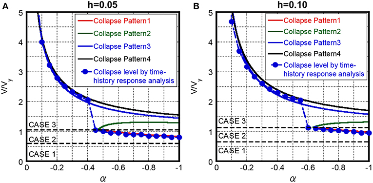
Figure 9. Comparison of proposed collapse-limit input velocity level and minimum collapse-limit input velocity level by time-history response analysis, (A) h = 0.05, (B) h = 0.10.
Transition of Collapse-Limit Input Velocity Level With Respect to Damping Ratio
The effect of damping ratio on the collapse-limit level of the critical double impulse is investigated here. Figure 10 shows the collapse level with respect to the post-yield stiffness ratio for three damping ratios h = 0.0, 0.05, 0.10. It should be pointed out again that the collapse-limit input velocity level corresponding to h = 0 was shown in Kojima and Takewaki (2016a). Figure 11 shows the transition of the collapse level in Collapse Patterns 1–4 for these three damping ratios. It can be understood from Figures 10, 11 that the collapse input level of Collapse Patterns 1–4 becomes larger and the region for Collapse Pattern 3 becomes wider, as the damping ratio becomes larger. For example, the collapse-limit input velocity level for α = −0.20 and h = 0.10 becomes larger than that for α = −0.20 and h = 0 by about 38 percent in Collapse Pattern 3.
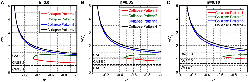
Figure 10. Collapse–limit input velocity level of critical double impulse with respect to post-yield stiffness ratio for specific damping ratio, (A) h = 0.0, (B) h = 0.05, (C) h = 0.10.
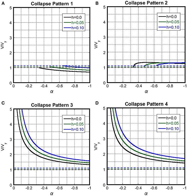
Figure 11. Input velocity level of Collapse Patterns 1–4 for specific damping ratio, (A) Collapse Pattern 1, (B) Collapse Pattern 2, (C) Collapse Pattern 3, (D) Collapse Pattern 4.
Applicability of the Proposed Collapse-Limit Input Level to the Corresponding One-Cycle Sinusoidal Wave
The applicability of the proposed collapse input level of the critical double impulse is investigated to the one-cycle sinusoidal wave which can represent the main-part of near-fault ground motions through the comparison with the collapse velocity level of the one-cycle sinusoidal wave. The following relation between the input velocity level V of the double impulse and the maximum velocity Vp of the corresponding one-cycle sinusoidal wave has been proposed based on the equivalence of the maximum Fourier amplitude (Kojima and Takewaki, 2016b; Kojima et al., 2017).
The maximum deformation to the critical one-cycle sinusoidal wave is evaluated by the time-history response analysis by changing the input wave period for the constant maximum velocity Vp and the collapse-limit input level V(= Vp/1.222) of the one-cycle sinusoidal wave is evaluated where the maximum deformation attains the collapse limit (the zero-restoring force point in the second stiffness range). The critical one-cycle sinusoidal wave indicates the one-cycle sinusoidal wave with the input wave period which maximizes the maximum deformation for the constant maximum velocity Vp.
Figure 12 shows the comparison of the proposed collapse level of the critical double impulse and the collapse input level of the one-cycle sinusoidal wave for the damping ratio h = 0.05, 0.10. The collapse level by the one-cycle sine wave for h = 0.05 corresponds to the proposed collapse level in Collapse Pattern 1 in the region α < −0.45 and corresponds to that in Collapse Pattern 3 in the region −0.45 < α < −0.2. The collapse level by the one-cycle sine wave corresponds to the proposed collapse level in Collapse Pattern 4 in the region α > −0.2. On the other hand, the collapse level of the one-cycle sinusoidal wave for h = 0.10 corresponds to the collapse level in Collapse Pattern 1 in the region α < −0.55 and corresponds to that in Collapse Pattern 3 in the region −0.55 < α < −0.2. The collapse level by the one-cycle sine wave corresponds to the proposed collapse level in Collapse Pattern 4 in the region α > −0.2. However, the proposed collapse input level provides a slightly dangerous one compared with the collapse level by the one-cycle sine wave in the region where the collapse level is determined by Collapse Pattern 3. The stable region between Collapse Pattern 2 and 3 exists only in the critical double impulse.
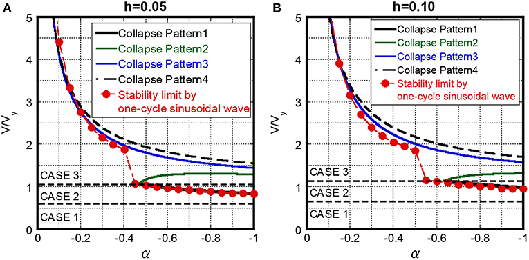
Figure 12. Comparison of proposed collapse-limit input velocity level of critical double impulse and collapse level of one-cycle sinusoidal wave, (A) h = 0.05, (B) h = 0.10.
Applicability of the Proposed Collapse-Limit Input Level to Actual Recorded Ground Motions
In order to investigate the validity of the double impulse as a substitute for near-fault ground motions and the applicability of the proposed theory to actual recorded ground motions, the time-history response analysis is conducted to actual recorded ground motions. Then the collapse level of actual recorded ground motions is investigated. In this paper, the Rinaldi station FN component during the 1994 Northridge earthquake and the Kobe University NS component during the 1995 Hyogoken-Nanbu earthquake are used as the representative near-fault ground motions. Figure 13 shows the accelerograms of the Rinaldi station FN component and the Kobe University NS component with their equivalent one-cycle sinusoidal waves. In this paper, the one-cycle sinusoidal wave which can represent the main part of the recorded ground motions is extracted and the extracted one-cycle sinusoidal wave is transformed into the double impulse with same manner in section Applicability of the Proposed Collapse-Limit Input Level to the Corresponding One-Cycle Sinusoidal Wave (Kojima and Takewaki, 2016b). The acceleration amplitude Ap(= πVp/Tp) and the period Tp of the one-cycle sinusoidal wave equivalent to the Rinaldi station FN component are Ap = 7.85[m/sec2] and Tp = 0.8[sec]. On the other hand, the acceleration amplitude and the period of the one-cycle sinusoidal wave equivalent to the Kobe University NS component are Ap = 2.60[m/sec2] and Tp = 1.0[sec]. The input velocity level of the double impulse corresponding to the Rinaldi station FN component is V = 1.64[m/sec] and that corresponding to the Kobe University NS component is V = 0.677[m/sec].
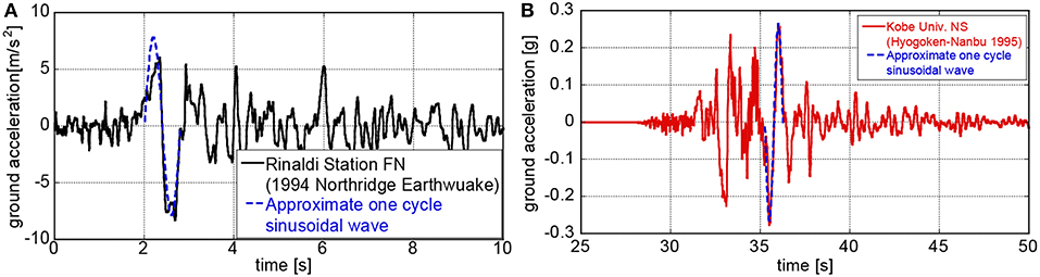
Figure 13. Actual recorded ground motions and equivalent one-cycle sine wave, (A) Rinaldi station FN component during 1994 Northridge earthquake, (B) Kobe University NS component during 1995 Hyogoken-Nanbu earthquake.
In above sections, the critical double impulse or the critical one-cycle sinusoidal wave has been determined for a certain input velocity level (or a certain maximum velocity). On the other hand, the critical elastic-plastic response under a given actual earthquake ground motion (fixed) for a certain structural parameter Vy(= ω1dy) is evaluated here by changing the natural circular frequency and the yield deformation (Kojima and Takewaki, 2016b; Kojima et al., 2017). This evaluation method has been explained in the literature (Kojima and Takewaki, 2016b; Kojima et al., 2017). Figure 14A shows the comparison of the maximum deformation of the system with h = 0.10 and α = −0.80 under the Rinaldi station FN component in the critical case and that under the critical double impulse with respect to V/Vy. From Figure 14A, the normalized collapse-limit level of the Rinaldi station FN component is V/Vy = 1.080 for h = 0.10 and α = −0.80. The collapse-limit level V/Vy = 1.080 of the Rinaldi station FN component is close to the collapse-limit level V/Vy = 1.058 evaluated by the proposed method in Collapse Pattern 1. Figures 14B–D present the restoring force-deformation relation, the normalized deformation time history and the normalized restoring-force time history for the stable case (V/Vy = 1.079) and the collapse case (V/Vy = 1.080). On the other hand, Figure 15A shows the comparison of the maximum deformation of the system with h = 0.05 and α = −0.60 under the Kobe University NS component in the critical case and that under the critical double impulse with respect to V/Vy. From Figure 15A, the normalized collapse-limit level of the Kobe University NS component is V/Vy = 0.949 for h = 0.05 and α = −0.60. The collapse-limit level V/Vy = 0.949 of the Kobe University NS component is close to the collapse-limit level V/Vy = 0.981 evaluated by the proposed method in Collapse Pattern 1. Figures 15B–D present the restoring force-deformation relation, the normalized deformation time history and the normalized restoring-force time history for the stable case (V/Vy = 0.948) and the collapse case (V/Vy = 0.949). It can be observed that the proposed theory provides a reasonably accurate collapse-limit velocity level.
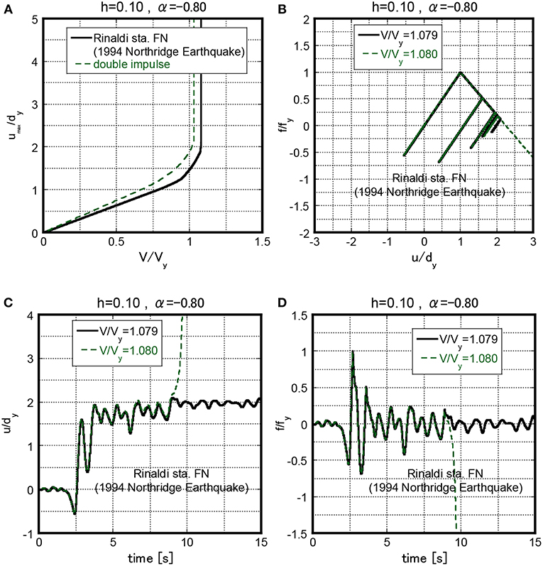
Figure 14. Elastic-plastic response under Rinaldi station FN component of system with h = 0.10, α = −0.80 for stable case (V/Vy = 1.079) and collapse case (V/Vy = 1.080), (A) Maximum deformation with respect to normalized input level, (B) Restoring force-deformation relation, (C) Normalized deformation time history, (D) Normalized restoring-force time history.
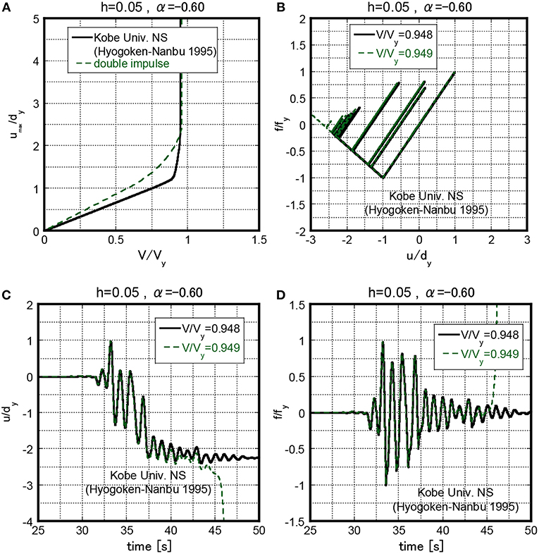
Figure 15. Elastic-plastic response under Kobe University NS component of system with h = 0.05, α = −0.60 for stable case (V/Vy = 0.948) and collapse case (V/Vy = 0.949), (A) Maximum deformation with respect to normalized input level, (B) Restoring force-deformation relation, (C) Normalized deformation time history, (D) Normalized restoring-force time history.
Conclusions
The double impulse has been introduced as a substitute for the fling-step near-fault ground motion and the approximate closed-form solution for the collapse-limit input velocity level of the critical double impulse has been derived for a damped bilinear hysteretic SDOF system with negative post-yield stiffness. The conclusions can be summarized as follows.
1. The collapse-limit input velocity level of the critical double impulse can be derived approximately by introducing the quadratic-function approximation of the damping force-deformation relation and the energy balance law. Since the critical timing of the second impulse had been proved to be the zero-restoring-force timing in the unloading process in the previous study (Kojima et al., 2017; Akehashi et al., 2018), it was used in this paper. In this theory, the collapse-limit input velocity level of the double impulse can be obtained as a function of the post-yield stiffness ratio and damping ratio. It may be important to emphasize again that, while the damping ratio has never been included in the collapse-limit input velocity level in the previous investigation for the undamped model, it is included explicitly in the present paper for the damped model. The accuracy of the proposed solution was investigated through the time-history response analysis for the stable and collapse models.
2. The applicability of the approximate solution for the collapse-limit input velocity level to near-fault ground motions was investigated through the comparison with the collapse-limit input velocity level of the one-cycle sinusoidal wave. The proposed solution can provide the collapse-limit input velocity level of near-fault ground motions with reasonable accuracy.
3. The applicability of the collapse-limit input velocity level to actual recorded ground motions was investigated through the time-history response analysis for the stable and collapse models under the Rinaldi station FN component during the 1994 Northridge earthquake and the Kobe University NS component during the 1995 Hyogo-ken Nanbu earthquake. It was confirmed that the proposed theory can evaluate the collapse level of these two earthquake ground motions with reasonable accuracy.
The proposed method enables a closed-form expression useful for the judgement of a stable or collapse state of a structure under earthquake ground motions. However, the readers should keep in mind again that the present theory is based on the following three assumptions: (a) the principal part of a near-fault ground motion can be simulated by a critical double impulse, (b) the critical timing of the second impulse taken equal to zero-restoring force timing after the first impulse is an assumption following (Kojima et al., 2017; Akehashi et al., 2018), (c) the damping force-deformation relation is approximated by a quadratic function. In addition, the modeling of a multi-storied building structure into a single-degree-of-freedom model treated in this paper appears important and critical. This issue will be discussed in the future research.
Data Availability
The datasets generated for this study are available on request to the corresponding author.
Author Contributions
YS formulated the problem, conducted the computation, and wrote the paper. KK conducted the computation, discussed the results, and wrote the paper. IT supervised the research and wrote the paper.
Funding
Part of the present work was supported by KAKENHI of Japan Society for the Promotion of Science (Nos. 15H04079, 17J00407, 17K18922, 18H01584). This support was greatly appreciated.
Conflict of Interest Statement
The authors declare that the research was conducted in the absence of any commercial or financial relationships that could be construed as a potential conflict of interest.
References
Adam, C., and Jager, C. (2012). “Dynamic instabilities of simple inelastic structures subjected to earthquake excitation,” in Advanced Dynamics and Model-Based Control of Structures and Machines, eds H. Irschik, M. Krommer, and A. K. Belyaev (Wien: Springer, 11–18.
Akehashi, H., Kojima, K., and Takewaki, I. (2018). Critical response of SDOF damped bilinear hysteretic system under double impulse as substitute for near-fault ground motion. Front. Built Environ. 4:5. doi: 10.3389/fbuil.2018.00005
Araki, Y., and Hjelmstad, K. D. (2000). Criteria for assessing dynamic collapse of elastoplastic structural systems. Earthquake Eng. Struct. Dyn. 29, 1177–1198. doi: 10.1002/1096-9845(200008)29:8<1177::AID-EQE963>3.0.CO;2-E
Bernal, D. (1987). Amplification factors for inelastic dynamic P-Δ effects in earthquake analysis. Earthquake Eng. Struct. Dyn. 15, 635–651. doi: 10.1002/eqe.4290150508
Bernal, D. (1992). Instability of buildings subjected to earthquakes. J. Struct. Eng. 118, 2239–2260.
Bernal, D. (1998). Instability of buildings during seismic response. Eng. Struct. 20, 496–502. doi: 10.1016/S0141-0296(97)00037-0
Bertero, V. V., Mahin, S. A., and Herrera, R. A. (1978). Aseismic design implications of near-fault San Fernando earthquake records. Earthquake Eng. Struct. Dyn. 6, 31–42. doi: 10.1002/eqe.4290060105
Casapulla, C. (2015). On the resonance conditions of rigid rocking blocks. Int. J. Eng. Tech. 7, 760–771.
Casapulla, C., and Maione, A. (2017). Critical response of free-standing rocking blocks to the intense phase of an earthquake. Int. Rev. Civil Eng. 8, 1–10. doi: 10.15866/irece.v8i1.11024
Challa, V. R. M., and Hall, J. F. (1994). Earthquake collapse analysis of steel frames. Earthquake Eng. Struct. Dyn. 23, 1199–1218. doi: 10.1002/eqe.4290231104
Chatzis, M. N., and Smyth, A. W. (2012). Robust modeling of the rocking problem. J. Eng. Mech. 138, 247–262. doi: 10.1061/(ASCE)EM.1943-7889.0000329
Ger, J.-F., Cheng, Y., and Lu, L.-W. (1993). Collapse behavior of Pino Suarez building during 1985 Mexico City earthquake. J. Struct. Eng. 119, 852–870. doi: 10.1061/(ASCE)0733-9445(1993)119:3(852)
Hall, J. F. (1998). Seismic response of steel frame buildings to near-source ground motions. Earthquake Eng. Struct. Dyn. 27, 1445–1464.
Herrmann, G. (Ed.). (1965). “Dynamic stability of structures,” in Proceedings of an International Conference Held at North Western University (Oxford: Pergamon Press).
Hjelmstad, K. D., and Williamson, E. B. (1998). Dynamic stability of structural systems subjected to base excitation. Eng. Struct. 20, 425–432. doi: 10.1016/S0141-0296(97)00034-5
Ibarra, L. F., and Krawinkler, H. (2005). Global Collapse of Frame Structures Under Seismic Excitations. PEER Center Report 2005/06. Richmond.
Ishida, S., and Morisako, K. (1985). Collapse of SDOF system to harmonic excitation. J. Eng. Mech. 111, 431–448.
Jennings, P. C., and Husid, R. (1968). Collapse of yielding structures during earth-quakes. J. Eng. Mech. 94, 1045–1065.
Khoshnoudian, F., Ahmadi, E., Kiani, M., and Tehrani, M. H. (2014). Short communication, collapse capacity of soil-structure systems under pulse-like earthquakes. Earthquake Eng. Struct. Dyn. 44, 481–490. doi: 10.1002/eqe.2501
Kojima, K., Saotome, Y., and Takewaki, I. (2017). Critical earthquake response of a SDOF elastic-perfectly plastic model with viscous damping under double impulse as a substitute of near-fault ground motion. J. Struct. Constr. Eng. 735, 643–652. doi: 10.3130/aijs.82.643
Kojima, K., and Takewaki, I. (2015). Critical earthquake response of elastic-plastic structures under near-fault ground motions (Part 1: fling-step input). Front. Built Environ. 1:12. doi: 10.3389/fbuil.2015.00012
Kojima, K., and Takewaki, I. (2016a). Closed-form dynamic stability criterion for elastic-plastic structures under near-fault ground motions. Front. Built Environ. 2:6. doi: 10.3389/fbuil.2016.00006
Kojima, K., and Takewaki, I. (2016b). Closed-form critical earthquake response of elastic-plastic structures with bilinear hysteresis under near-fault ground motions. J. Struct. Constr. Eng. 726, 1209–1219. doi: 10.3130/aijs.81.1209
Maier, G., and Perego, U. (1992). Effects of softening inelastic-plastic structural dynamics. Int. J. Numer. Methods Eng. 34, 319–347. doi: 10.1002/nme.1620340120
Makris, N., and Vassiliou, M. F. (2013). Planar rocking response and stability analysis of an array of free-standing columns capped with a freely supported rigid beam. Earthquake Eng. Struct. Dyn. 42, 431–449. doi: 10.1002/eqe.2222
Miranda, E., and Akkar, S. D. (2003). Dynamic instability of simple structural systems. J. Struct. Eng. 129, 1722–1726. doi: 10.1061/(ASCE)0733-9445(2003)129:12(1722)
Nabeshima, K., Taniguchi, R., Kojima, K., and Takewaki, I. (2016). Closed-form overturning limit of rigid block under critical near-fault ground motions. Front. Built Environ. 2:9. doi: 10.3389/fbuil.2016.00009
Nakajima, A., Abe, H., and Kuranishi, S. (1990). Effect of multiple collapse modes on dynamic failure of structures with structural instability. Struct. Eng. Earthquake Eng. 7, 1s−11s.
Sasani, M., and Bertero, V. V. (2000). “Importance of severe pulse-type ground motions in performance-based engineering: historical and critical review,” in Proceedings of the Twelfth World Conference on Earthquake Engineering (Auckland).
Sivaselvan, M. V., Lavan, O., Dargush, G. F., Kurino, H., Hyodo, Y., Fukuda, R., et al. (2009). Numerical collapse simulation of large-scale structural systems using an optimization-based algorithm. Earthquake Eng. Struct. Dyn. 38, 655–677. doi: 10.1002/eqe.895
Sun, C.-K., Berg, G. V., and Hanson, R. D. (1973). Gravity effect on single-degree inelastic system. J. Eng. Mech. Div. 99, 183–200.
Takizawa, H., and Jennings, P. C. (1980). Collapse of a model for ductile reinforced concrete frames under extreme earthquake motions. Earthquake Eng. Struct. Dyn. 8, 117–144. doi: 10.1002/eqe.4290080204
Tanabashi, R., Nakamura, T., and Ishida, S. (1973). “Gravity effect on the catastrophic dynamic response of strain-hardening multi-story frames,” in Proceedings of 5th World Conference on Earthquake Engineering (Rome), 2140–2149.
Uetani, K., and Tagawa, H. (1998). Criteria for suppression of deformation concentration of building frames under severe earthquakes. Eng. Struct. 20, 372–383. doi: 10.1016/S0141-0296(97)00021-7
Williamson, E. B., and Hjelmstad, K. D. (2001). Nonlinear dynamics of a harmonically-excited inelastic inverted pendulum. J. Eng. Mech. 127, 52–57. doi: 10.1061/(ASCE)0733-9399(2001)127:1(52)
Appendix Analysis for Collapse Pattern 3
Detailed derivation of the quartic equation of V/Vy for Collapse Pattern 3 is explained here.
From Figure 5, the plastic deformation up3 after experiencing the maximum deformation after the second impulse can be obtained from −fy − αkup1 + αkup2 − αkup3 = 0.
This means that the maximum deformation after experiencing the closed loop just attains the collapse limit in the same direction as the maximum deformation after the first impulse. Then, up3 can be obtained by
where up1 in Equation (A1) can be obtained from Equation (18). up2 can be derived from the following energy balance law between the point at the second impulse (Point C in Figure 5) and the point at the maximum deformation after the second impulse (Point E in Figure 5) (Akehashi et al., 2018).
From Equation (A2), up2/dy can be derived by
where vc can be obtained by Equation (15).
The velocity ṽ in Equation (22) can be obtained by solving the equation of motion in the unloading process after experiencing the maximum deformation −umax 2 (Point E in Figure 5) after the second impulse. The equation of motion in the unloading process (between Point E and Point G in Figure 5) can be expressed by
The displacement, velocity, and acceleration responses can be computed by solving Equation (A4) and substituting at the transition point (Point E).
In Equations (A5a–c), t = 0 was set at Point E. From Equation (A5a), the timing tv max when becomes maximum can be obtained as and the velocity ṽ can be obtained by substituting tv max into Equation (A5b).
With the notation λ = (− αup1 + αup2)/dy and Equation (A6), Equation (22) can be transformed into the following equation.
where . From Equation (A7), λ is obtained as
By substituting up1 by Equation (18) and up2 by Equation (A3) into λ = (− αup1 + αup2)/dy, the following equation can be derived.
where 1 − αup1/dy = I, (vc + V)/Vy = J.
From Equation (15) and the notation , is obtained and the following equation can be derived by substituting into Equation (A9).
Equation (A10) can be transformed into
By substituting Equation (18) and I = 1 − αup1/dy into Equation (A11), the following equation can be obtained.
Define K, L, M, N, O as follows.
By substituting Equations (A13a–d) into Equation (A12) and arranging the equation, the following equation can be obtained.
Here, N and O can be transformed as follows.
where P = (8/3)h(1 − α) − 2αC, Q = (16/3)h(1 − α)C − 4αC2 + (8/3)hC(λ + 1), R = 4Cα − (8/3)h(λ + 1), S = 4C2α − (λ + 1)2 − (16/3)h(λ + 1)C.
By substituting Equations (A13a,b), (A15a,b) into Equation (A14), the following quartic equation can be derived.
where
The input velocity level V/Vy in Collapse Pattern 3 can be computed by solving the Equation (A16). Then, the collapse-limit level has to be a real number and satisfy Inequality (9).
Keywords: earthquake response, critical excitation, double impulse, collapse, bilinear hysteresis, viscous damping
Citation: Saotome Y, Kojima K and Takewaki I (2019) Collapse-Limit Input Level of Critical Double Impulse for Damped Bilinear Hysteretic SDOF System With Negative Post-yield Stiffness. Front. Built Environ. 5:106. doi: 10.3389/fbuil.2019.00106
Received: 18 May 2019; Accepted: 26 August 2019;
Published: 18 September 2019.
Edited by:
Nikos D. Lagaros, National Technical University of Athens, GreeceReviewed by:
Paolo Castaldo, Polytechnic University of Turin, ItalyClaudia Casapulla, University of Naples Federico II, Italy
Aristotelis E. Charalampakis, National Technical University of Athens, Greece
Copyright © 2019 Saotome, Kojima and Takewaki. This is an open-access article distributed under the terms of the Creative Commons Attribution License (CC BY). The use, distribution or reproduction in other forums is permitted, provided the original author(s) and the copyright owner(s) are credited and that the original publication in this journal is cited, in accordance with accepted academic practice. No use, distribution or reproduction is permitted which does not comply with these terms.
*Correspondence: Izuru Takewaki, takewaki@archi.kyoto-u.ac.jp