 Francesco Bardi1,2,3†
 Emanuele Gasparotti1†
 Emanuele Vignali1†
 Maria Nicole Antonuccio1,2
 Eleonora Storto1
 Stéphane Avril1
 Simona Celi1*
- 1BioCardioLab, Bioengineering Unit, Ospedale del Cuore, Massa, Italy
- 2Mines Saint-Étienne, Université Jean Monnet, INSERM, Saint Étienne, France
- 3Predisurge, Grande Usine Creative 2, Saint Étienne, France
Background: Cardiovascular diseases remain a leading cause of morbidity and mortality worldwide and require extensive investigation through in-vitro studies. Mock Circulatory Loops (MCLs) are advanced in-vitro platforms that accurately replicate physiological and pathological hemodynamic conditions, while also allowing for precise and patient-specific data collection. Particle Image Velocimetry (PIV) is the standard flow visualization technique for in-vitro studies, but it is costly and requires strict safety measures. High-power Light Emitting Diode illuminated PIV (LED-PIV) offers a safer and cheaper alternative.
Methods: In this study, we aim to demonstrate the feasibility of a Hybrid-MCL integrated with a LED-PIV system for the investigation of Abdominal Aortic Aneurysm (AAA) compliant phantoms. We considered two distinct AAA models, namely, an idealized model and a patient-specific one under different physiological flow and pressure conditions.
Results: The efficacy of the proposed setup for the investigation of AAA hemodynamics was confirmed by observing velocity and vorticity fields across multiple flow rate scenarios and regions of interest.
Conclusion: The findings of this study underscore the potential impact of Hybrid-MCL integrated with a LED-PIV system on enhancing the affordability, accessibility, and safety of in-vitro CVD investigations.
1 Introduction
In vitro studies play a crucial role in cardiovascular disease (CVD) research, as they represent a great alternative to animal models (Celi et al., 2022) and can serve as a reliable means to validate in silico methods.
Incorporating 3D models (Garcia et al., 2018) into a mock-circulatory loop (MCL) system offers the in-vitro test-bench solution to reproduce physiological and pathological conditions with patient-specific accuracy in terms of both geometry and hemodynamics in a fully controlled environment. Indeed, MCLs allow for the collection of precise and patient-specific data, thus providing valuable insights into biological flows that can significantly enhance our knowledge of CVDs. MCLs have been extensively used not only to test cardiovascular devices such as heart valves (Hasler and Obrist, 2018) and LVADs (Ochsner et al., 2013; Zimpfer et al., 2016; Chassagne et al., 2021), but also to study the complex fluid dynamics inside blood vessels (Kefayati and Poepping, 2013; Bonfanti et al., 2020; Mariotti et al., 2023).
In this context, Particle Image Velocimetry (PIV) (Raffel et al., 2018) is the reference flow visualization method that provides high spatial and temporal resolutions and has been used to validate in-vivo measurement techniques (Roloff et al., 2019). However, a standard PIV setup entails substantial costs, both in terms of initial purchase and ongoing operation and maintenance. The main cost is due to the illumination source, which is a high-power double-pulse laser, either Nd:YAG or Nd:YAF (Raffel et al., 2018). In addition, special training is required to safely operate these laser systems (classified as Class 4 lasers) as they can cause permanent blindness or skin burns.
To address these challenges, alternative illumination sources have been explored (Cierpka et al., 2021; Caridi et al., 2022), with light-emitting diodes (LEDs) emerging as a promising solution. LEDs offer a safer, more cost-effective alternative to traditional lasers, with the added benefit of easier handling and reduced maintenance costs. The feasibility of using LEDs for PIV was first demonstrated by Willert et al. (2010), who developed an electronic circuitry capable of operating LEDs with high-pulsed currents. Their work showed that by using pulse widths as short as 20
In this work, we seek, for the first time, to extend the application of LED-PIV to the study AAAs fluid dynamics. Our primary objective is to demonstrate the feasibility of using LED-PIV for investigating the hemodynamics of large vessels. We specifically focused on the abdominal aorta as a test case due to the intricate flow dynamics induced by the presence of an aneurysm. To achieve this, we employed a Hybrid Mock Circulatory Loop (HMCL) combined with LED-PIV. HMCLs (Ochsner et al., 2013; Cappon et al., 2021; Bardi et al., 2023) distinguish themselves from traditional MCLs by incorporating an active numerical-hydraulic module, which allows for continuous and interactive tuning of the pressure boundary conditions. This capability is particularly useful when working with deformable phantoms derived from patient-specific geometries. By integrating the advanced control capabilities of the HMCL with the LED-PIV setup, we present a novel approach for investigating AAA hemodynamics. Through validating the effectiveness of LED-PIV in this context, we aim to highlight its broader potential in cardiovascular research, particularly in enabling safer and more cost-effective experimental studies.
2 Methods
2.1 Fabrication of AAA models
Two deformable transparent models of AAA morphology were manufactured using the “lost-mold casting”: an idealized axial-symmetric AAA model and a patient-specific AAA model. This process consisted in 3D-printing internal and external molds in a water-soluble material, which were dissolved in hot water once the casting material had cured. Each step involved in the lost-mold casting is described in detail in Antonuccio et al. (2023) and is summarized herein.
The manufacturing process comprised six key steps: i) model creation; ii) mold design; iii) 3D-printing of the molds; iv) surface treatment; v) material casting; vi) removal of the molds. The idealized axial-symmetric AAA model was developed based on a geometry employed in Salsac et al. (2006a) for fabricating rigid models. Two geometrical parameters define the AAA shape: 1) the aspect ratio
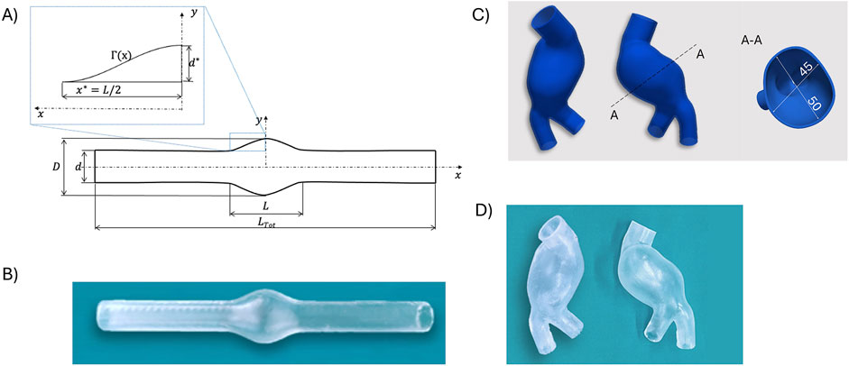
Figure 1. Representations of the idealized axial-symmetric model (A) and the associated deformable phantom (B). CAD representations of the patient-specific AAA model (C) and associated patient-specific phantom (D).
Figure 1A depicts the CAD representation of the idealized axial-symmetric AAA model.
Regarding the patient-specific model, computed tomography scans of a patient with AAA were segmented to reconstruct the 3D vessel geometry, including the abdominal aorta, aneurysm bulge, and left/right iliac (Antonuccio et al., 2023). The segmented geometry was exported as a stereo-lithography format file, converted into a solid model, and further processed in SOLIDWORKS (Dassault Systèmes S. A., Vélizy-Villacoublay, France) to design molds using the same approach for both AAA models.
A wall thickness of 1.8 mm was obtained by applying an outward offset to the inner surface of the models. A core and two outer molds were designed for material casting. The core, defining the inner surface, featured a hollow design with 15 mm reference pins at inlets and outlets.
Outer molds, defining the outer surface, were created through a multi-step process involving the creation of a monolithic external mold, splitting it into two counterparts, making the outer molds hollow by subtracting the core and solid model, and designing sprues, reference pins, and gluing channels.
All molds were 3D-printed using a fused deposition modeling printer (A4v3, 3NTR Italy) with a 2.85 mm polyvinyl alcohol (PVA) filament. PVA, a water-soluble material, dissolved upon curing of the casting material. Before casting, mold surfaces in contact with the casting material underwent treatment to eliminate roughness. Molds were assembled, closed firmly, and cast with two-component silicone Sylgard 184 (Dow, Wiesbaden, Germany), known for its compliant properties, which are suitable for vascular district fabrication for optical applications Yazdi et al. (2018). The material’s compliance aligns with the elasticity range of the human aorta, which varies between 0.25 MPa and 1.7 MPa, as reported by Lang et al. (1994). After silicone curing for 48 h at room temperature, the PVA components dissolved by immersing the molds in warm water in an ultrasonic tank. Four washing cycles, including a 1-h ultrasound-enabled cycle at 60°C, were performed. The dissolved PVA left a smooth lumen and a smooth exterior surface. The resulting deformable transparent models were subsequently soaked in cold water for finalization (Figures 1C, D).
2.2 Mock circulatory loop
A flow circuit was assembled to replicate physiological hemodynamic conditions inside the phantoms. A sketch of the circuit is shown in Figure 2.
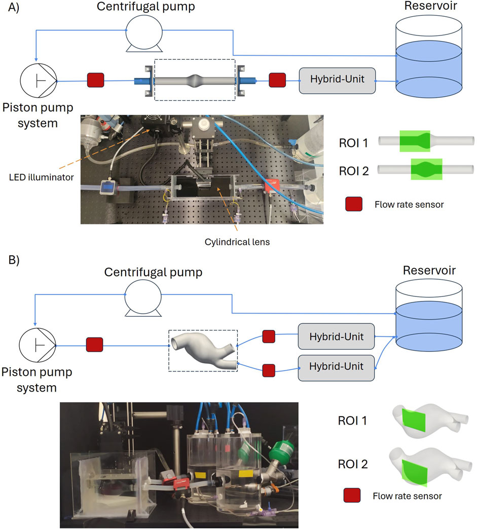
Figure 2. Hybrid Mock Circulatory Loop set up for the idealized AAA model (A) and for the patient-specific AAA model (B).
A versatile piston pump, previously presented in Vignali et al. (2022), along with a mechanical heart valve, was used to generate a pulsatile flow rate. The outlets of the phantoms were connected to pressure-regulated chambers (hybrid units), designed to replicate Windkessel effect. Each hybrid unit, as detailed in Bardi et al. (2023), consists of an acrylic cylindrical chamber where the pressure is pneumatically controlled by solenoid valves connected to a vacuum (−0.5 kPa) and a pressure line (3 kPa). The pressure, measured at the bottom of the chamber, is regulated by a PID controller. The setpoint pressure is dynamically computed at each time step based on the latest flow rate measurement, following a 3-Element Windkessel (3WKM) model. Considering that the aortic model was assumed to be at diastolic pressure, the Windkessel parameters (proximal resistance
A CompactRIO controller (cRIO-9047, NI) was used to control the system and to acquire the sensor data. Clamp-on ultrasonic flow meters (Sonoflow CO.55/100 V2.0 - CO.55/190 V2.0, Sonotec) were used to measure the flow rates at the inlet and the outlets of the AAA models. The gains of each ultrasonic flow meter were calibrated by using the encoder of the piston pump, with the same working fluid under pulsatile flow conditions; a delay ranging between 20 ms and 26 ms was found. The pressure inside the hybrid units was monitored through IFM Electronic PA3509 sensors and additional clinical pressure transducers (TruWave, Edwards) were used to monitor the inlet and outlet pressures. All data were logged with a frequency of 5 kHz.
2.3 PIV setup
A mixture composed of 60% of glycerol and 40% of water can be used to match the refractive index of Sylgard. However, 22% of urea was added to water - glycerol mixture (62/38) to also maintain the density
The LED pulse-width
The four setting configurations are.
For each experiment, 50 cardiac cycles were reproduced, and the last 25 cycles were used to acquire the images, namely, 25 images per cardiac cycle (31 ms between each image pair).
Two specific regions of interest (ROIs) were considered for each model, i.e., one proximal to the inlet
2.4 Experimental test cases
For the patient-specific AAA model, Doppler-echographic in-vivo flow measurements were used to define the flow profile
where
These parameters, along with the 3WKM parameters for the outlet boundary conditions for each flow profile are reported in Table 1.
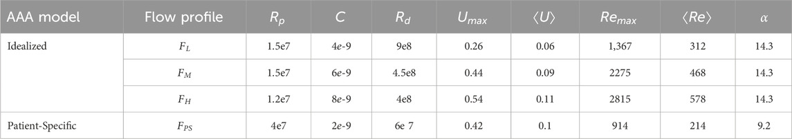
Table 1. 3WKM parameters, velocity, Reynolds and Womersley numbers for each flow profile.
2.5 Data processing
The flow and pressure sensors data were low-pass filtered with a cutoff frequency of 25 kHz. The acquired 25 cycles were considered to obtain a phase average and the corresponding standard deviation. The difference between the flow rate at the inlet and the sum of the outlets was also computed. Concerning the PIV image analysis, a specific pre-processing was applied to enhance the quality of the cross-correlation and to improve the subsequent velocity reconstruction. In particular, the following operations were imposed: background subtraction, intensity rescaling, equalization via contrast limited adaptive histogram processing (CLAHE), Gaussian filtering and edge extraction. In particular, the background was evaluated by starting from the average image and subtracted to the original for each ROI. Then, the intensity of the image was scaled between the 20th and 99.5 percentile of the intensity values to extract the inner edges of the phantom. Subsequently, CLAHE and a Gaussian filter were applied to improve the contrast and reduce the noise. At last, the edges of the phantom in each ROI were manually initialized, and then, an accurate segmentation was performed through an active contour algorithm. The results in terms of image pre-processing for each ROI are presented in Figure 3. The obtained contours were finally used to mask the images and to evaluate the deformation of the phantoms at three different longitudinal locations
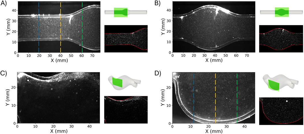
Figure 3.
Given the limited field of view,
After image processing, the velocity field was computed using the open-source software OpenPIV (Liberzon et al., 2020; Ben-Gida et al., 2020). The velocity field was calculated using the FFT-based correlation algorithm with a window deformation approach, which involved 3 passes and interrogation areas of 128 × 128, 64 × 64 and 32 × 32 pixels with a 50% overlap. The image resolution for the idealized AAA model and the patient-specific one were 24.6 px/mm and 41.6 px/mm, respectively. The vector validation process consisted of verifying that the global velocity threshold (set at five times the standard deviation) and the local median threshold (set at three times the median) were met. Additionally, the validation ensured that the signal-to-noise ratio was above a value of 1.25. The rate of invalid vectors detected through this process ranged between 0.5% and 3% for the idealized model and between 1% and 9.5% for the patient-specific model.
3 Results
3.1 Idealized AAA model
The flow rates measured at the inlet and outlet sections for the three test cases (
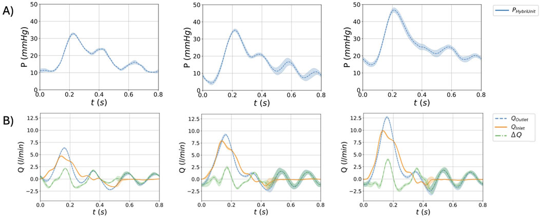
Figure 4. Waveforms for the idealized AAA model for the three flow conditions
Table 2 summarises the
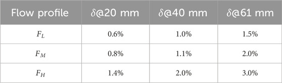
Table 2. Deformation parameter
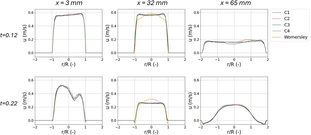
Figure 5. Phase averaged axial velocity profiles
For the
Figure 6 shows the differences between the PIV setting configurations with respect to
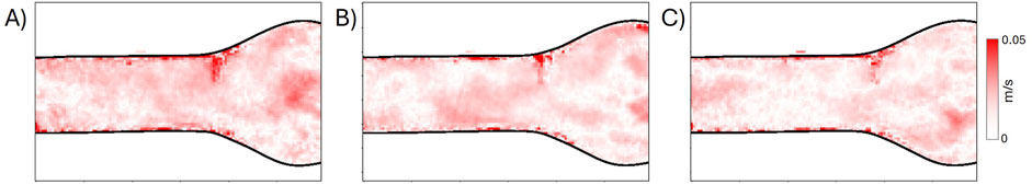
Figure 6. Differences of the velocity field at the systolic peak for the
Figures 7A, 8 present the velocity vectors and the velocity magnitude fields for each flow condition. Five time-frames (at 0.06, 0.12, 0.22, 0.28, and 0.46 s), obtained under the
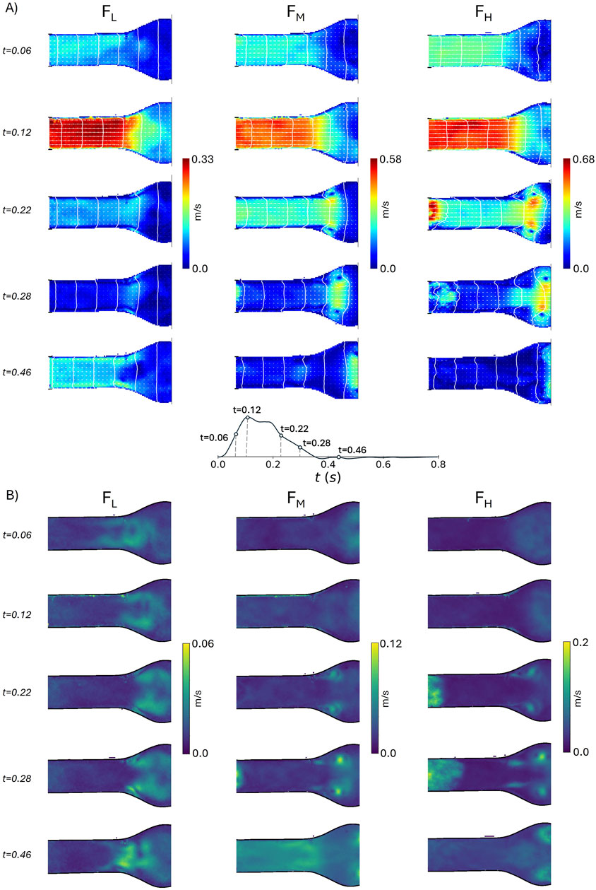
Figure 7. Velocity magnitude field with velocity vectors (A) and root mean square of velocity fluctuations (B) in the idealized model at
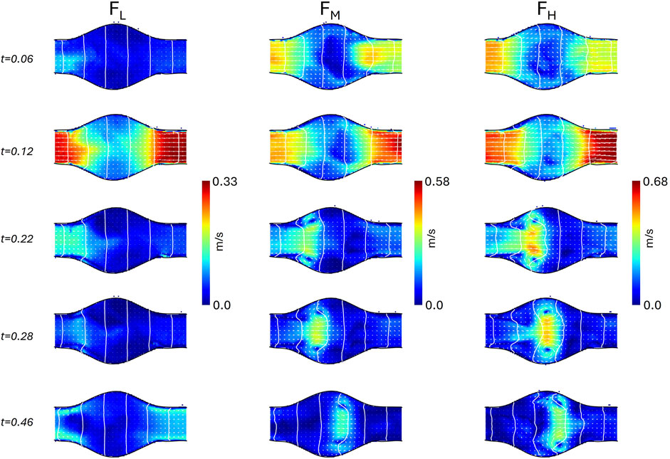
Figure 8. Velocity magnitude field with velocity vectors in the idealized model at
Analogously, the vorticity magnitude field is shown in Figures 9, 10, for
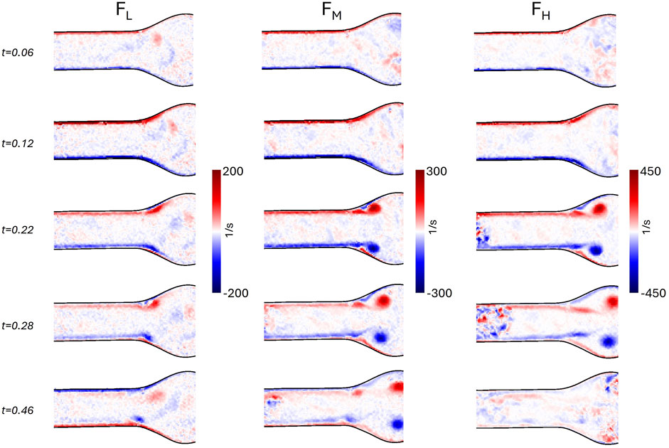
Figure 9. Vorticity field in the idealized model at
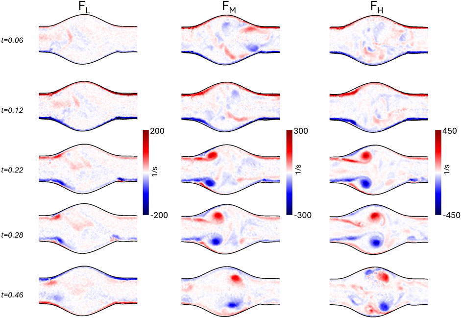
Figure 10. Vorticity field in the idealized model at
The longitudinal component of the velocity at the inlet of
where
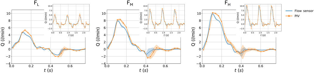
Figure 11. Comparison between the sensor measured flow rate, and the PIV derived flow rate, for the three flow rate conditions
3.2 Patient-specific AAA model
Figure 12 depicts the phase-averaged waveforms of the flow rates at inlet, outlets and their balance; the pressure in the hybrid units, and deformations at three different longitudinal locations on
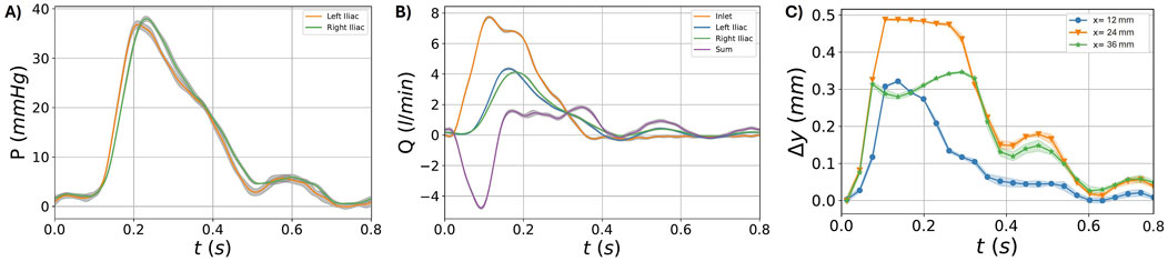
Figure 12. Waveforms for the patient-specific model. Pressure in the two hybrid units (A). Flow rate at the inlet, outlets (left and right iliac), and and their difference
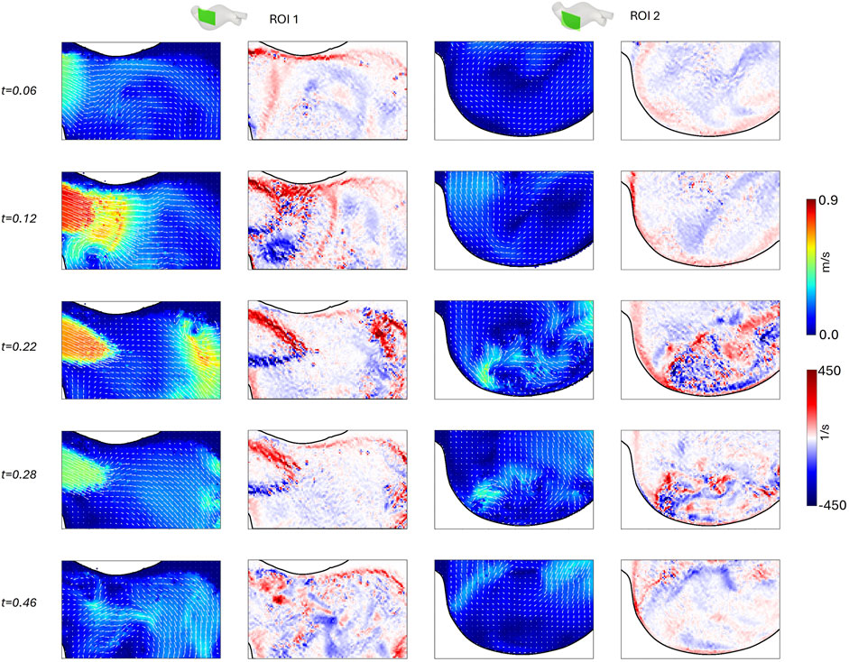
Figure 13. Velocity magnitude field with velocity vectors and vorticity field for
4 Discussion and conclusion
MCL systems have gained increasing popularity in the experimental analysis of cardiovascular systems due to their ability to replicate hemodynamic conditions with high fidelity (Zimmermann et al., 2021; Vignali et al., 2022; Agrafiotis et al., 2024). Integrating a high-fidelity HMCL with a PIV system serves two crucial purposes. Firstly, it provides a comprehensive benchmark for validating in silico data from numerical approaches (Mariotti et al., 2020; Lan et al., 2022; Fanni et al., 2023). Secondly, this setup can be used to gain new insights by replicating in-vitro multiple hemodynamic conditions as observed in clinical environments and is a valuable tool for enhancing the accuracy of other velocity reconstruction methods, such as Color-Doppler imaging (Antonuccio et al., 2022). Additional value is added when a compliant phantom is used to mimic patient-specific cardiovascular conditions (Fanni et al., 2020; Wu et al., 2022; Antonuccio et al., 2023; Moravia et al., 2023) for a deeper understanding of hemodynamic parameters such as pressure, flow, velocity fields, and vessel deformation.
The integrated PIV-HMCL system presented in this work is particularly effective due to its ability to operate under controlled and highly reproducible pressure conditions, enabled by using hybrid chambers (Bardi et al., 2023). Moreover, the feasibility of using a high-power LED-PIV system promotes the spread of in-vitro studies in cardiovascular research (Cierpka et al., 2021; Torta et al., 2024). Our low-cost setup significantly reduces the investment required by conventional PIV systems up to approximately one hundred thousand euros by eliminating the need for dedicated high-speed cameras, high-energy laser sources, and specialized PIV synchronization units. The choice of an LED light source offers the crucial advantage of being safer and less hazardous than lasers used in traditional PIV systems, which require specific precautions and procedures as envisaged by the international standard IEC 60825–1.
This study is the first to explore the feasibility of low-cost LED-PIV measurements for the in-vitro characterization of abdominal aorta flows under fully controlled patient-specific pulsatile flow and pressure conditions. Specifically, testing was conducted on both an idealized AAA model and a patient-specific one.
Concerning the idealized model, Figure 4 represents the results in terms of flow, pressure, and deformations. In particular, the results demonstrate that the HMCL could replicate three different fluid dynamic conditions, both in terms of pressure and flow (Figures 4A, B) waveforms. The obtained pressure values were consistent with the physiological range of pressures in the abdominal aorta (Amanuma et al., 1992). Moreover, the results demonstrate the system’s repeatability, given the standard deviation range observed in the plots. The phantom’s deformability is responsible for differences between inlet and outlet flow waveforms. These effects were quantified by the
Concerning the effect of the illumination settings on the velocity obtained from the PIV data processing, the four configurations tested did not reveal relevant differences. This is evident from the three axial velocity profiles of Figure 5 for the
Although the geometry of the idealized AAA model is the same as the geometry presented in Salsac et al. (2006b), and similar Reynolds and Womersley numbers were used, a point-wise quantitative comparison of velocity and vorticity fields is not feasible. Indeed, we imposed different systole-to-diastole time ratios, the backflow was only due to the regurgitation of the heart valve, and the phantom was flexible. Nonetheless, it is possible to qualitatively compare the velocity (Figures 7, 8) and the vorticity (Figures 9, 10) fields. In particular, the flow field of
According to Yip and Yu (2001), this flow regime, also observed in
Finally, the flow rate calculated from the axial velocity and the flow rate measured with the sensor (Figure 11) were found consistent for all three flow rate conditions. The maximum error was found to be less than 2 L/min. For all flow conditions, there is a visible difference at peak systole. This difference is likely due to the velocity being taken 3 cm from the rigid adapter, where the inlet flexible part acts as a compliance. Other discrepancies could be due to the inaccurate hypothesis of perfectly axial symmetrical flow and the accuracy of the flow sensors in measuring flow rates, especially for lower flow rates.
Considering then the patient-specific model, the waveforms of Figure 12 (A) show a physiological behavior in terms of pressures. Moreover, by observing the mean and standard deviation values of pressure, we can confirm the reproducibility of the pressure conditions prescribed by the HMCL. As already observed in the AAA model, the
Additionally, the thickness of the light sheet and light reflections constrained the choice of acquiring planes. In the case of complex geometry such as the one of this study, the definition of a suitable PIV plane is not a trivial task due to the light incidence on the curved surface (Ronneberger et al., 1998; Edwards et al., 2020). As shown in Figures 3C,D, a noticeable reflection was observed in the patient-specific model despite the CLAHE filtering. This blurring effect likely compromised the accuracy of the velocity field reconstruction, making the results in the small region near the curved wall unreliable. The issue of spurious reflections could potentially be mitigated by using fluorescent particles combined with an appropriate filter.
This work showed that high-power LED-illuminated PIV is a viable and affordable alternative to a standard laser PIV system to study large blood vessels’ hemodynamic in-vitro. LED-PIV is safe to use in both educational/training and clinical settings. In the CVD research context, as numerical models keep gaining importance, the need for accurate and reliable results has become increasingly more relevant (Viceconti et al., 2021; Lan et al., 2022). The present study addresses this need by providing experimental data that can be used to evaluate and refine numerical models.
Data availability statement
The raw data supporting the conclusions of this article will be made available by the corresponding author upon reasonable request.
Author contributions
FB: Conceptualization, Data curation, Formal Analysis, Investigation, Methodology, Software, Validation, Visualization, Writing–original draft, Writing–review and editing. EG: Conceptualization, Formal Analysis, Investigation, Methodology, Resources, Software, Visualization, Writing–original draft, Writing–review and editing. EV: Conceptualization, Formal Analysis, Investigation, Methodology, Resources, Software, Visualization, Writing–original draft, Writing–review and editing. MA: Data curation, Formal Analysis, Investigation, Writing–review and editing. ES: Data curation, Investigation, Writing–review and editing. SA: Conceptualization, Funding acquisition, Project administration, Supervision, Writing–review and editing. SC: Conceptualization, Funding acquisition, Project administration, Resources, Supervision, Visualization, Writing–original draft, Writing–review and editing.
Funding
The author(s) declare that financial support was received for the research, authorship, and/or publication of this article. This project has received funding from the European Union’s Horizon 2020 research and innovation program under the Marie SkłodowskaCurie grant agreement No 859836.
Conflict of interest
Author FB was employed by company Predisurge. The remaining authors declare that the research was conducted in the absence of any commercial or financial relationships that could be construed as a potential conflict of interest.
The reviewer DO declared a past co-authorship with the authors SC and EV to the handling editor.
Publisher’s note
All claims expressed in this article are solely those of the authors and do not necessarily represent those of their affiliated organizations, or those of the publisher, the editors and the reviewers. Any product that may be evaluated in this article, or claim that may be made by its manufacturer, is not guaranteed or endorsed by the publisher.
Supplementary material
The Supplementary Material for this article can be found online at: https://www.frontiersin.org/articles/10.3389/fbioe.2024.1452278/full#supplementary-material
References
Agrafiotis, E., Zimpfer, D., Mächler, H., and Holzapfel, G. A. (2024). Review of systemic mock circulation loops for evaluation of implantable cardiovascular devices and biological tissues. J. Endovascular Ther., 15266028241235876. doi:10.1177/15266028241235876
Amanuma, M., Mohiaddin, R., Hasegawa, M., Heshiki, A., and Longmore, D. (1992). Abdominal aorta: characterisation of blood flow and measurement of its regional distribution by cine magnetic resonance phase-shift velocity mapping. Eur. Radiol. 2, 559–564. doi:10.1007/bf00187552
Antonuccio, M. N., Gasparotti, E., Bardi, F., Monteleone, A., This, A., Rouet, L., et al. (2023). Fabrication of deformable patient-specific aaa models by material casting techniques. Front. Cardiovasc. Med. 10, 1141623. doi:10.3389/fcvm.2023.1141623
Antonuccio, M. N., Morales, H. G., This, A., Capellini, K., Avril, S., Celi, S., et al. (2022). Towards the 2D velocity reconstruction in abdominal aorta from Color-Doppler Ultrasound. Med. Eng. & Phys. 107, 103873. doi:10.1016/j.medengphy.2022.103873
Bardi, F., Gasparotti, E., Vignali, E., Avril, S., and Celi, S. (2023). A hybrid mock circulatory loop for fluid dynamic characterization of 3D anatomical phantoms. IEEE Trans. Biomed. Eng. 70, 1651–1661. doi:10.1109/TBME.2022.3224581
Bauer, A., Bopp, M., Jakirlic, S., Tropea, C., Krafft, A. J., Shokina, N., et al. (2020). Analysis of the wall shear stress in a generic aneurysm under pulsating and transitional flow conditions. Exp. Fluids 61, 59. doi:10.1007/s00348-020-2901-4
Ben-Gida, H., Gurka, R., and Liberzon, A. (2020). OpenPIV-MATLAB – an open-source software for particle image velocimetry; test case: birds’ aerodynamics. SoftwareX 12, 100585. doi:10.1016/j.softx.2020.100585
Bonfanti, M., Franzetti, G., Homer-Vanniasinkam, S., Díaz-Zuccarini, V., and Balabani, S. (2020). A combined in vivo, in vitro, in silico approach for patient-specific haemodynamic studies of aortic dissection. Ann. Biomed. Eng. 48, 2950–2964. doi:10.1007/s10439-020-02603-z
Bracco, M. I., Broda, M., Lorenzen, U. S., Florkow, M. C., Somphone, O., Avril, S., et al. (2023). Fast strain mapping in abdominal aortic aneurysm wall reveals heterogeneous patterns. Front. Physiology 14, 1163204. doi:10.3389/fphys.2023.1163204
Brindise, M. C., Busse, M. M., and Vlachos, P. P. (2018). Density- and viscosity-matched Newtonian and non-Newtonian blood-analog solutions with PDMS refractive index. Exp. Fluids 59, 173. doi:10.1007/s00348-018-2629-6
Buchmann, N. A., Willert, C. E., and Soria, J. (2012). Pulsed, high-power LED illumination for tomographic particle image velocimetry. Exp. Fluids 53, 1545–1560. doi:10.1007/s00348-012-1374-5
Cappon, F., Wu, T., Papaioannou, T., Du, X., Hsu, P.-L., and Khir, A. W. (2021). Mock circulatory loops used for testing cardiac assist devices: a review of computational and experimental models. Int. J. Artif. Organs 44, 793–806. doi:10.1177/03913988211045405
Caridi, G. C. A., Torta, E., Mazzi, V., Chiastra, C., Audenino, A. L., Morbiducci, U., et al. (2022). Smartphone-based particle image velocimetry for cardiovascular flows applications: a focus on coronary arteries. Front. Bioeng. Biotechnol. 10, 1011806. doi:10.3389/fbioe.2022.1011806
Celi, S., Cioffi, M., Capellini, K., Fanni, B. M., Gasparotti, E., Vignali, E., et al. (2022). Advanced non-animal models in biomedical research
Chassagne, F., Miramontes, M., Chivukula, V. K., Li, S., Beckman, J. A., Mahr, C., et al. (2021). In vitro investigation of the effect of left ventricular assist device speed and pulsatility mode on intraventricular hemodynamics. Ann. Biomed. Eng. 49, 1318–1332. doi:10.1007/s10439-020-02669-9
Chen, C.-Y., Antón, R., Hung, M.-y., Menon, P., Finol, E. A., and Pekkan, K. (2014). Effects of intraluminal thrombus on patient-specific abdominal aortic aneurysm hemodynamics via stereoscopic particle image velocity and computational fluid dynamics modeling. J. Biomechanical Eng. 136, 031001. doi:10.1115/1.4026160
Cierpka, C., Otto, H., Poll, C., Hüther, J., Jeschke, S., and Mäder, P. (2021). SmartPIV: flow velocity estimates by smartphones for education and field studies. Exp. Fluids 62, 172. doi:10.1007/s00348-021-03262-z
Deplano, V., Guivier-Curien, C., and Bertrand, E. (2016). 3D analysis of vortical structures in an abdominal aortic aneurysm by stereoscopic PIV. Exp. Fluids 57, 167. doi:10.1007/s00348-016-2263-0
Deplano, V., Knapp, Y., Bailly, L., and Bertrand, E. (2014). Flow of a blood analogue fluid in a compliant abdominal aortic aneurysm model: experimental modelling. J. Biomechanics 47, 1262–1269. doi:10.1016/j.jbiomech.2014.02.026
Derwich, W., Keller, T., Filmann, N., Schmitz-Rixen, T., Blasé, C., Oikonomou, K., et al. (2023). Changes in aortic diameter and wall strain in progressing abdominal aortic aneurysms. J. Ultrasound Med. 42, 1737–1746. doi:10.1002/jum.16193
Edwards, M., Theunissen, R., Allen, C. B., and Poole, D. J. (2020). On the feasibility of selective spatial correlation to accelerate convergence of piv image analysis based on confidence statistics. Exp. Fluids 61, 222. doi:10.1007/s00348-020-03050-1
Egelho, C. J., Budwig, R. S., Elger, D. F., Khraishi, T. A., and Johansen, K. H. (1999). Model studies of the #ow in abdominal aortic aneurysms during resting and exercise conditions. J. Biomechanics. doi:10.1016/S0021-9290(99)00134-7
Fanni, B., Sauvage, E., Celi, S., Norman, W., Vignali, E., Landini, L., et al. (2020). A proof of concept of a non-invasive image-based material characterization method for enhanced patient-specific computational modeling. Cardiovasc. Eng. Technol. 11, 532–543. doi:10.1007/s13239-020-00479-7
Fanni, B. M., Gasparotti, E., Vignali, E., Capelli, C., Positano, V., and Celi, S. (2023). An integrated in-vitro and in-silico workflow to study the pulmonary bifurcation hemodynamics. Comput. & Fluids 260, 105912. doi:10.1016/j.compfluid.2023.105912
Garcia, J., Yang, Z., Mongrain, R., Leask, R. L., and Lachapelle, K. (2018). 3d printing materials and their use in medical education: a review of current technology and trends for the future. BMJ Simul. & Technol. Enhanc. Learn. 4, 27–40. doi:10.1136/bmjstel-2017-000234
Geoghegan, P. H., Buchmann, N. A., Soria, J., and Jermy, M. C. (2013). Time-resolved PIV measurements of the flow field in a stenosed, compliant arterial model. Exp. Fluids 54, 1528. doi:10.1007/s00348-013-1528-0
Hasler, D., and Obrist, D. (2018). Three-dimensional flow structures past a bio-prosthetic valve in an in-vitro model of the aortic root. PLOS ONE 13, e0194384. doi:10.1371/journal.pone.0194384
Kefayati, S., and Poepping, T. L. (2013). Transitional flow analysis in the carotid artery bifurcation by proper orthogonal decomposition and particle image velocimetry. Med. Eng. & Phys. 35, 898–909. doi:10.1016/j.medengphy.2012.08.020
Lan, I. S., Liu, J., Yang, W., Zimmermann, J., Ennis, D. B., and Marsden, A. L. (2022). Validation of the reduced unified continuum formulation against in vitro 4D-flow MRI. Ann. Biomed. Eng. 51, 377–393. doi:10.1007/s10439-022-03038-4
Lang, R. M., Cholley, B. P., Korcarz, C., Marcus, R. H., and Shroff, S. G. (1994). Measurement of regional elastic properties of the human aorta. a new application of transesophageal echocardiography with automated border detection and calibrated subclavian pulse tracings. Circulation 90, 1875–1882. doi:10.1161/01.CIR.90.4.1875
Liberzon, A., Käufer, T., Bauer, A., Vennemann, P., Zimmer, E., et al. (2020). OpenPIV/openpiv-python: openPIV - Python (v0.22.2) with a new extended search PIV grid option. doi:10.5281/zenodo.3930343
Mariotti, A., Vignali, E., Gasparotti, E., Capellini, K., Celi, S., and Salvetti, M. V. (2020). Comparison between numerical and mri data of ascending aorta hemodynamics in a circulatory mock loop. CINECA IRIS Institutional Res. Inf. Syst. 24, 898–907. doi:10.1007/978-3-030-41057-5_73
Mariotti, A., Vignali, E., Gasparotti, E., Morello, M., Singh, J., Salvetti, M. V., et al. (2023). In vitro analysis of hemodynamics in the ascending thoracic aorta: sensitivity to the experimental setup. Appl. Sci. 13, 5095. doi:10.3390/app13085095
Moravia, A., Simoëns, S., El Hajem, M., Bou-Saïd, B., Kulisa, P., Della-Schiava, N., et al. (2022). In vitro flow study in a compliant abdominal aorta phantom with a non-Newtonian blood-mimicking fluid. J. Biomechanics 130, 110899. doi:10.1016/j.jbiomech.2021.110899
Moravia, A., Simoëns, S., El Hajem, M., Bou-Saïd, B., Menut, M., Kulisa, P., et al. (2023). Particle image velocimetry to evaluate pulse wave velocity in aorta phantom with the ln d–u method. Cardiovasc. Eng. Technol. 14, 141–151. doi:10.1007/s13239-022-00642-2
Ochsner, G., Amacher, R., Amstutz, A., Plass, A., Schmid Daners, M., Tevaearai, H., et al. (2013). A novel interface for hybrid mock circulations to evaluate ventricular assist devices. IEEE Trans. Biomed. Eng. 60, 507–516. doi:10.1109/TBME.2012.2230000
Raffel, M., Willert, C. E., Scarano, F., Kähler, C. J., Wereley, S. T., and Kompenhans, J. (2018). Particle image velocimetry: a practical guide. Cham: Springer International Publishing. doi:10.1007/978-3-319-68852-7
Roloff, C., Stucht, D., Beuing, O., and Berg, P. (2019). Comparison of intracranial aneurysm flow quantification techniques: standard PIV vs stereoscopic PIV vs tomographic PIV vs phase-contrast MRI vs CFD. J. NeuroInterventional Surg. 11, 275–282. doi:10.1136/neurintsurg-2018-013921
Ronneberger, O., Raffel, M., and Kompenhans, J. (1998). “Advanced evaluation algorithms for standard and dual plane particle image velocimetry,” in Proceedings of the 9th international symposium on applications of laser techniques to fluid mechanics (Lisbon, Portugal), 13–16.
Salsac, A.-V., Sparks, S., Chomaz, J.-M., and Lasheras, J. (2006a). Evolution of the wall shear stresses during the progressive enlargement of symmetric abdominal aortic aneurysms. J. Fluid Mech. 560, 19–51. doi:10.1017/s002211200600036x
Salsac, A.-V., Sparks, S. R., Chomaz, J.-M., and Lasheras, J. C. (2006b). Evolution of the wall shear stresses during the progressive enlargement of symmetric abdominal aortic aneurysms. J. Fluid Mech. 560, 19. doi:10.1017/S002211200600036X
Stamatopoulos, C., Mathioulakis, D. S., Papaharilaou, Y., and Katsamouris, A. (2011). Experimental unsteady flow study in a patient-specific abdominal aortic aneurysm model. Exp. Fluids 50, 1695–1709. doi:10.1007/s00348-010-1034-6
Torta, E., Griffo, B., Caridi, G. C., De Nisco, G., Chiastra, C., Morbiducci, U., et al. (2024). Smartphone-based particle tracking velocimetry for the in vitro assessment of coronary flows. Med. Eng. & Phys. 126, 104144. doi:10.1016/j.medengphy.2024.104144
Viceconti, M., Pappalardo, F., Rodriguez, B., Horner, M., Bischoff, J., and Tshinanu, F. M. (2021). In silico trials: verification, validation and uncertainty quantification of predictive models used in the regulatory evaluation of biomedical products. Methods 185, 120–127. doi:10.1016/j.ymeth.2020.01.011
Vignali, E., Gasparotti, E., Mariotti, A., Haxhiademi, D., Ait-Ali, L., and Celi, S. (2022). High-versatility left ventricle pump and aortic mock circulatory loop development for patient-specific hemodynamic in vitro analysis. ASAIO J. 68, 1272–1281. doi:10.1097/MAT.0000000000001651
Willert, C., Stasicki, B., Klinner, J., and Moessner, S. (2010). Pulsed operation of high-power light emitting diodes for imaging flow velocimetry. Meas. Sci. Technol. 21, 075402. doi:10.1088/0957-0233/21/7/075402
Wilson, K. A., Lee, A. J., Lee, A. J., Hoskins, P. R., Fowkes, F. R., Ruckley, C., et al. (2003). The relationship between aortic wall distensibility and rupture of infrarenal abdominal aortic aneurysm. J. Vasc. Surg. 37, 112–117. doi:10.1067/mva.2003.40
Wu, X., Gürzing, S., Schinkel, C., Toussaint, M., Perinajová, R., van Ooij, P., et al. (2022). Hemodynamic study of a patient-specific intracranial aneurysm: comparative assessment of tomographic piv, stereoscopic piv, in vivo mri and computational fluid dynamics. Cardiovasc. Eng. Technol. 13, 428–442. doi:10.1007/s13239-021-00583-2
Yazdi, S. G., Geoghegan, P. H., Docherty, P. D., Jermy, M., and Khanafer, A. (2018). A review of arterial phantom fabrication methods for flow measurement using PIV techniques. Ann. Biomed. Eng. 46, 1697–1721. doi:10.1007/s10439-018-2085-8
Yip, T. H., and Yu, S. C. M. (2001). Cyclic transition to turbulence in rigid abdominal aortic aneurysm models. Fluid Dyn. Res. 29, 81–113. doi:10.1016/S0169-5983(01)00018-1
Zimmermann, J., Loecher, M., Kolawole, F. O., Bäumler, K., Gifford, K., Dual, S. A., et al. (2021). On the impact of vessel wall stiffness on quantitative flow dynamics in a synthetic model of the thoracic aorta. Sci. Rep. 11, 6703. doi:10.1038/s41598-021-86174-6
Zimpfer, D., Strueber, M., Aigner, P., Schmitto, J. D., Fiane, A. E., Larbalestier, R., et al. (2016). Evaluation of the HeartWare ventricular assist device Lavare cycle in a particle image velocimetry model and in clinical practice. Eur. J. Cardio-Thoracic Surg. 50, 839–848. doi:10.1093/ejcts/ezw232
Keywords: LED-PIV, hemodynamics, mock circulatory loop, abdominal aortic aneurysm, aortic phantom, 3D-printing
Citation: Bardi F, Gasparotti E, Vignali E, Antonuccio MN, Storto E, Avril S and Celi S (2024) A hybrid mock circulatory loop integrated with a LED-PIV system for the investigation of AAA compliant phantoms. Front. Bioeng. Biotechnol. 12:1452278. doi: 10.3389/fbioe.2024.1452278
Received: 20 June 2024; Accepted: 25 September 2024;
Published: 10 October 2024.
Edited by:
Seungik Baek, Michigan State University, United StatesReviewed by:
Vanessa Diaz, University College London, United KingdomDominik Obrist, University of Bern, Switzerland
Copyright © 2024 Bardi, Gasparotti, Vignali, Antonuccio, Storto, Avril and Celi. This is an open-access article distributed under the terms of the Creative Commons Attribution License (CC BY). The use, distribution or reproduction in other forums is permitted, provided the original author(s) and the copyright owner(s) are credited and that the original publication in this journal is cited, in accordance with accepted academic practice. No use, distribution or reproduction is permitted which does not comply with these terms.
*Correspondence: Simona Celi, cy5jZWxpQGZ0Z20uaXQ=
†These authors have contributed equally to this work and share first authorship