Weighted fast-trimmed likelihood estimator for mixture regression models

The fast-trimmed likelihood estimate is a robust method to estimate the parameters of a mixture regression model. However, this method is vulnerable to the presence of bad leverage points, which are outliers in the direction of independent variables. To address this issue, we propose the weighted fast-trimmed likelihood estimate to mitigate the impact of leverage points. The proposed method applies the weights of the minimum covariance determinant to the rows suspected of containing leverage points. Notably, both real data and simulation studies were considered to determine the efficiency of the proposed method compared to the previous methods. The results reveal that the weighted fast-trimmed estimate method is more robust and reliable than the fast-trimmed likelihood estimate and the expectation–maximization (EM) methods, particularly in cases with small sample sizes.

Introduction

The mixture regression model has been widely used in various scientific fields, such as econometrics, engineering, biology, and others, due to its ability to capture the relationship between independent and dependent variables. As noted by Quandt (1) and Quandt and Ramsay (2), datasets may exhibit multiple data patterns, and variables often cluster according to these patterns. These patterns can be represented by unknown groups of latent variables, leading to the use of mixture regression models. In other words, the regression probabilistic model, in terms of the latent class variable Z, where Z = k, can be expressed as follows:

$\begin{array}{ll}Y=x\text{'}{\beta }_k+e_k,k=1,2,\dots ,g\text{,}& (1)\end{array}$

where $\mathrm{x}$ is the design matrix of $\left(p+1\right)$ independent variables with constant, and ${\beta }_k$is the regression parameters of $g\text{,}$ which is the number of homogeneous sub-populations (groups). Moreover, $e_k$ is the error term that has to be independent of $\mathrm{x}$ with density $f_k\left(.\right)\text{,}$ which is distributed $N\left(0,{\sigma }_k^2\right)\text{,}$ and $Y$ is the dependent variable, which has the same distribution of $e_k$ with different parameters.

The maximum likelihood estimation (MLE) method, widely regarded as one of the best methods to estimate regression model parameters when the distribution of errors is normal, becomes challenging when this assumption is violated. Moreover, MLE lacks robustness in the presence of outliers. Alternative methods should prioritize both ease of computation and robustness, such as the M-estimate (3) and the least trimmed squares method (4). These robust approaches address contaminated error distributions through two key procedures: first, fitting a parametric model to the majority distribution and removing errors following a different distribution; second, assigning reduced weights to outliers so they approximate a normal distribution. In some cases, the random errors are highly heterogeneous, with at least 50% of the errors lacking homogeneity (5).

Dempster et al. (6) introduced the expectation–maximization (EM) algorithm, which simplifies the problem by transforming it into a relatively straightforward single-component MLE. The EM algorithm is robust against outliers and easy to calculate. This issue of robustness in mixture regression models has garnered significant attention in statistical research. Initial efforts to address the problem of outliers in mixture models, particularly within the location-scale family of distributions, were made by Peel and McLachlan (7) and Hennig (8). In a different approach, Markatou (9), Neykov et al. (5), and Shen et al. (10) sought to mitigate the influence of outliers in mixture regression models by assigning reduced weights to individual data points.

Alternatively, Hadi and Luceño (11) and Vandev and Neykov (12) defined the weighted trimmed likelihood estimator (WTLE):

$\begin{array}{ll}\underset{\beta \in {\Theta }^P}{min}{\displaystyle \sum }_{i=1}^h{w}_{v\left(i\right)}f\left(y_{v\left(i\right)};\beta \right)=\underset{I\in I_h}{min}\underset{\beta \in {\Theta }^P}{min}{\displaystyle \sum }_{i=1}^h{w}_i\left[-log\phi \left(y_i;\beta \right)\right]\text{,}& (2)\end{array}$

where $f\left(y_{v\left(1\right)};\beta \right)\le f\left(y_{v\left(2\right)};\beta \right)\le \cdots \le f\left(y_{v\left(n\right)};\beta \right)$ for fixed $\beta ,I_h=C_h^n$ is the all-possible subsets of size $h$ that can be fitted by MLE and randomly selected from $n$ observations, $\phi \left(y_i;\beta \right)$ is the probability density function. ${\widehat{\beta }}_{\mathit{WTLE}}$ is given the subset with the minimal negative log-likelihood. However, Equation 2 accommodates for the number of estimators, MLE when $n=h$ , TLE when $w_{v\left(i\right)}=1,i=1,2,\dots ,n\text{,}$ the median likelihood estimator (MedLE) when $w_{v\left(h\right)}=1$ and $w_{v\left(i\right)}=0$ for $i\ne h\text{.}$ Both MedLE and trimmed likelihood estimator (TLE) can coincide with other estimators depending on the definition of the density function $\phi \left(y_i;\beta \right)$ ; when it is multivariate normal, the MedLE and TLE correspond with minimum volume ellipsoid (MVE) and minimum covariance determinant (MCD) estimators (4). When it is normal density, the MedLE and TLE correspond to the least median of squares (LMS) and least trimmed squares (LTS). Neykov et al. (5) highlighted that WTLE is not a practical choice for large datasets and introduced the fast-trimmed likelihood estimate (FTLE) algorithm as a developed version of the approach originally proposed by Müller and Neykov (13). FTLE reduces Fast-LTS and Fast-MCD (14) in computing mixture regression coefficients in two steps, trial and refinement, respectively.

However, FTLE is not resistant in the presence of bad leverage points, which are outliers in the direction of independent variables. Garcia-Escudero et al. (15) proposed an adaptive procedure to identify the real cluster regressions without the influence of bad leverage points. Despite the increase in the second trimming in the breakdown point, it does not necessarily have high efficiency due to the high percentage of trimming, which reduces the degrees of freedom and, consequently, results in a loss of efficiency. Uraibi (16) employed the weights that are derived from re-weighted multivariate normal (RMVN), which is a robust location and scatter matrix proposed by Olive and Hawkins (17), instead of removing the outliers. This study suggests weighting the leverage points in the design matrix X using RMVN prior to using it with the TLE algorithm that deals with outliers in the y-direction.

Weighted fast-trimmed likelihood estimator

The FTLE method is not a feasible choice with moderate and small sizes due to the twice trimming for outliers and leverage points. This procedure leads to a loss of more information and consequently reduces the degrees of freedom. Thus, assigning down weights for leverage points instead of removing them might improve the performance of the TLE method. Moreover, identifying the percentage of outliers will contribute to the fast computation of TLE in the framework of the C-steps concentrated algorithm.

Uraibi (16) noted that the Fast MVE and MCD methods proposed by Rousseeuw and Driessen (14) are time-consuming and susceptible to masking and swamping phenomena when high leverage points are present. Consequently, using robust Mahalanobis distance based on MVE or MCD to identify leverage points may not be effective, as it can lead to inaccurate diagnostics regarding the exact number of leverage points. Uraibi (16) suggested using RMVN location and scale estimators (17) with Mahalanobis distance instead of MVE and MCD, as RMVN is a more concentrated algorithm and provides higher accuracy. Moreover, it is more resistant to high leverage points than other methods Uraibi and Haraj (18). Additionally, Uraibi (16) proposed an alternative weighting method that adjusts the chi-square distribution’s percentage point to address the masking and swamping problems caused by high leverage points. This approach is essential in the proposed algorithm for assigning high-accuracy weights to mitigate the issue of high leverage points.

Consider $F\left(e\right)$ as a scale mixture normal distribution of random errors term of Equation 1, where $F\left(e\right)=\left(1-\in \right)N\left(0,{\sigma }^2\right)+\in G$ . In this study, $G$ is another distribution different from $N\left(0,{\sigma }^2\right)$ and $\in \ge 0.25\text{.}$ Assume that $\left(n\times \alpha \right)$ leverage points are present in each independent variable, where $\alpha$ is the percentage of leverage points. The WTLE algorithm combines the weights algorithm of Uraibi (16) but uses RMVN (17) and the FTLE method in one algorithmic frame that can be written as follows:

1. Identifying leverage points and giving them down weights as follows:

For $j=1,2$ Do {

a. Compute ${\widehat{\mu }}_{\mathit{RMVN}}$ and ${\widehat{{\displaystyle \sum }}}_{\mathit{RMVN}}$ , the location and scatter estimators of $\mathrm{x}$ , and consider that the critical value of the desired upper bound of Mahalanobis distance is ${\chi }_{\left(0.975,p\right)}^2$ .

b. Calculate Robust Mahalanobis distance, which is denoted as $RD\left({\mathrm{x}}_i\right)$ based on ${\widehat{\mu }}_{\mathit{RMVN}}$ and ${\widehat{{\displaystyle \sum }}}_{\mathit{RMVN}}$ , $RD\left({\mathrm{x}}_i\right)={\left({\mathrm{x}}_i-{\widehat{\mu }}_{\mathit{RMVN}}\right)}^{\prime }{\widehat{{\displaystyle \sum }}}_{\mathit{RMVN}}^{-1}\left({\mathrm{x}}_i-{\widehat{\mu }}_{\mathit{RMVN}}\right)$ .

c. Let $S={\displaystyle \sum }_{i}Rd\left({\mathrm{x}}_i\right)$ where $Rd\left({\mathrm{x}}_i\right)=\left\{RD\left({\mathrm{x}}_i\right):RD\left({\mathrm{x}}_i\right)\le {\chi }_{\left(0.975,p\right)}^2\right\}$ .

d. Suppose that $\delta =\frac{\left(0.975\times n\right)}{2\times S}$ and $q=min\left(\delta ,0.995\right)\text{,}$ and then

${\widehat{{\displaystyle \sum }}}_{RM\left(j\right)}=\left[\mathit{Median}\left(RD\left({\mathrm{x}}_i\right)\right)/{\chi }_{\left(\delta ,p\right)}^2\right]\times {\widehat{{\displaystyle \sum }}}_{\mathit{RMVN}}\text{.}$

e. Let ${\widehat{{\displaystyle \sum }}}_{\mathit{RMVN}}={\widehat{{\displaystyle \sum }}}_{RM\left(j\right)}$ .

f. Next }.

g. Finally, $w_i=min\left[1,\frac{{\chi }_{\left(q,p\right)}^2}{RD\left({\mathrm{x}}_i\right)}\right]$ and then ${\mathrm{x}\mathrm{w}}_i={\mathrm{x}}_i\times w_i$ , $Y_{Wi}=Y_i\times w_i$ .

2. Identifying the number of outliers in $Y_W$ using robust three-sigma rules to determine the percentage of outliers ( $\alpha )$ that so-called the trimming value, the C-steps can be written as follows:

Random select $h$ out of $n$ such that $h=n\left(1-\alpha \right)$ .

a. Given $H^{\mathit{old}}:=\left\{Y_{W\left(1\times h\right)}\subset Y_{W\left(1\times n\right)}\right\}$ with corresponding $:=\left\{{\mathrm{x}\mathrm{w}}_{\left(h\times p+1\right)}\subset {\mathrm{x}\mathrm{w}}_{\left(n\times p+1\right)}\right\}$ and then compute ${\widehat{\beta }}_w^{\mathit{old}}$using multiple runs of MLE for mixture regression based on $H^{\mathit{old}}$ .

b. Let $Q^{\mathit{old}}:={\displaystyle \sum }_{i=1}^{h}f\left(y_i,{\widehat{\beta }}_w^{\mathit{old}}\right)$ and then sort.

c. $f\left(y_i,{\widehat{\beta }}_w^{\mathit{old}}\right)$ in ascending order $f\left(y_{\pi \left(i\right)},{\widehat{\beta }}_w^{\mathit{old}}\right)\le$ $f\left(y_{\pi \left(i+1\right)},{\widehat{\beta }}_w^{\mathit{old}}\right)$ .

d. Get the permutation $\pi =\left(\pi \left(1\right),\pi \left(2\right),\dots ,\pi \left(n\right)\right)\mathrm{t}$ .

e. Obtain $H^{\mathit{new}}:=\left\{y_{\pi \left(1\right)},y_{\pi \left(2\right)},\dots ,y_{\pi \left(h\right)}\right\}$ .

f. ${\widehat{\beta }}_w^{\mathit{new}}:=MLE$ based on $H^{\mathit{new}}$ .

g. $Q^{\mathit{new}}:={\displaystyle \sum }_{i=1}^{h}f\left(y_{\pi \left(i\right)},{\widehat{\beta }}_w^{\mathit{new}}\right)$ .

h. If $\frac{\left|Q^{\mathit{old}}-Q^{\mathit{new}}\right|}{Q^{\mathit{new}}}<\delta \text{,}$ stop; otherwise, repeat the steps (3–5) until convergence, where $\delta$ is a very small value.

Simulation study

This section describes a simulation study prepared to examine the performance of the proposed algorithm WFTLE compared to EM and FTLE methods.

Consider the mixture linear regression model as follows:

$Y=\{\begin{array}{cc}{\theta }_0+{\theta }_1{X}_1+{\theta }_2{X}_2+e,& \mathit{if}Z=1\\ {\theta }_0-{\theta }_1{X}_1-{\theta }_2{X}_2+e& \mathit{if}Z=2\end{array}\text{,}$

where $Z$ is the latent variable and when $P\left(Z=1\right)$ is construct ${\pi }_1=0.25$ of the components of $Y$ and $P\left(Z=2\right)$ is constructed $\left({\pi }_2=1-{\pi }_1\right)$ . The $X_1$and $X_2$ are sampled independently and are identically distributed from standard normal distribution individually with $n=\left\{25,50,75,100,200,500\right\}\text{.}$ The error terms $e$has been considered in the context of the following cases:

$X_1=100,X_2=100.$

I. Let the initial values are ${\theta }_i=\left\{\begin{array}{ccc}{\beta }_1=\left(1,2,2\right)& \sigma =1& {\pi }_1=0.25\\ {\beta }_2=\left(1,-2,-2\right)& \sigma =1& {\pi }_2=0.75\end{array}\right\}$ , generate $n$ data points from the standard normal distribution, $e~N\left(0,1\right)$and the computing $Y$ .

II. Generate $n$ data points from a uniform distribution such that $e=\left\{\begin{array}{cc}N\left(0,1\right)& \mathrm{if}u\le 0.90\\ N\left(5,1\right)& \mathrm{if}u>0.90\end{array}\right\}$ , and then finding $Y=\left\{\begin{array}{cc}1+2X_1+2X_2+e& \mathrm{if}u\le \pi \\ 1-2X_1-2X_2+e& \mathrm{if}u>\pi \end{array}\right\}$ , where $\pi =0.25$ of the components of $Y$ .

III. The same procedure as case II, with 10% of leverage points being in $X_1=100,X_2=100$ .

IV. Generate $n$ data points from a uniform distribution such that $e=\left\{\begin{array}{cc}N\left(0,1\right)& \mathrm{if}u\le 0.90\\ N\left(0,5^2\right)& \mathrm{if}u>0.90\end{array}\right\}$ and calculate $Y$ .

V. The same procedure as case IV, with 10% of leverage points being in:

The steps (I-V) are repeated 5,000 times, and the mean squares errors of the estimated component are computed as follows:

$Mse\left({\widehat{\theta }}_i\right)=\frac{{{\displaystyle \sum }}_{j=1}^{5000}{\left({\widehat{\theta }}_i-{\theta }_i\right)}^2}{5000},i=1,2\text{,}$

$\mathit{Bias}\left({\widehat{\theta }}_i\right)=\frac{{{\displaystyle \sum }}_{j=1}^{5000}|{\widehat{\theta }}_i-{\theta }_i|}{5000},i=1,2\text{,}$

$Mse\left({\widehat{\sigma }}_i\right)=\frac{{{\displaystyle \sum }}_{j=1}^{5000}{\left({\widehat{\sigma }}_i-1\right)}^2}{5000},i=1,2.$

The best method is the one that has the lowest values of the above criteria.

It is interesting to note regarding the results of case I of the simulation study reported in Table 1 when the distribution of random errors is standard normal. The values of $Mse\left({\widehat{\theta }}_j\right)$ , $\mathit{Bias}\left({\widehat{\theta }}_j\right)$ , and (between two parentheses in the tables) $Mse\left({\widehat{\sigma }}_i\right)$of the EM method, where $j=1,2,3$ respectively, are lowest than their counterparts in FTLE and WFTLE methods when $n=\left(25,50,75\right)$ . Notably, the values of $Mse\left({\widehat{\theta }}_j\right)$ become smaller little by little when the size $n$ increases from 25 to 500. Moreover, the values of $\mathit{Bias}\left({\widehat{\theta }}_i\right)$ are very small and coincide with $Mse\left({\widehat{\theta }}_i\right)$ values increase from 25 to 75, which is very close to each other where $n\to 500$ . The results of $Mse\left({\widehat{\sigma }}_i\right)$ in Table 1 are reasonable, and the performance of EM is better than the others when dealing with a small sample size since the algorithm of EM does not include any trimming procedure.

Table 1

Table 1. $Mse\left({\widehat{\theta }}_i\right)$, $\mathit{Bias}\left({\widehat{\theta }}_i\right)$, and $Mse\left({\widehat{\sigma }}_i\right)$ for case I of the simulation study.

Table 2 shows the simulation results of case II when the distribution of random errors is a mixture of normal; one is standard normal, and the other is shifted only by the mean. The results shown in this table suggest that the performance of FTLE and WFTLE methods is better than the EM method by having lower $Mse\left({\widehat{\theta }}_j\right)$ . Similarly, the WFTLE method is more efficient than the FTLE method when $n=\left\{25,50\right\}$ . Notably, both methods are very close when $n\ge 75$ . Regarding $\mathit{Bias}\left({\widehat{\theta }}_i\right)$ , FTLE and WFTLE methods produce the smallest bias than the EM method, but both are unstable with small samples of $n=\left\{25,50\right\}$ and have approximately the same results when $n\ge 75$ . It is clear that $Mse\left({\widehat{\sigma }}_i\right)$ of FTLE and WFTLE are better than the EM method with different sample sizes. However, FTLE is the best only when $n=25$ . This outperforms FTLE with this sample size not appearing with $\mathit{Bias}\left({\widehat{\theta }}_1\right)$ and $\mathit{Bias}\left({\widehat{\theta }}_2\right)\text{,}$ except $\mathit{Bias}\left(0\right)$ . It is notable that the $\mathit{Bias}\left({\widehat{\theta }}_1\right)$ and $\mathit{Bias}\left({\widehat{\theta }}_2\right)$ are the same when $n>25$ .

Table 2

Table 2. $Mse\left({\widehat{\theta }}_i\right)$, $\mathit{Bias}\left({\widehat{\theta }}_i\right)$, and $Mse\left({\widehat{\sigma }}_i\right)$ for case II of the simulation study.

Table 3 presents the results of three methods in the presence of leverage points for the data generated by case III of the simulation. Indeed, the performance of the WFTLE method is more efficient than others even when the sample size is $n=\left\{25,50,75\right\}$ , as summarized in Table 3. When the sample size is $n\ge 100\text{,}$ both methods have approximately the same performance.

Table 3

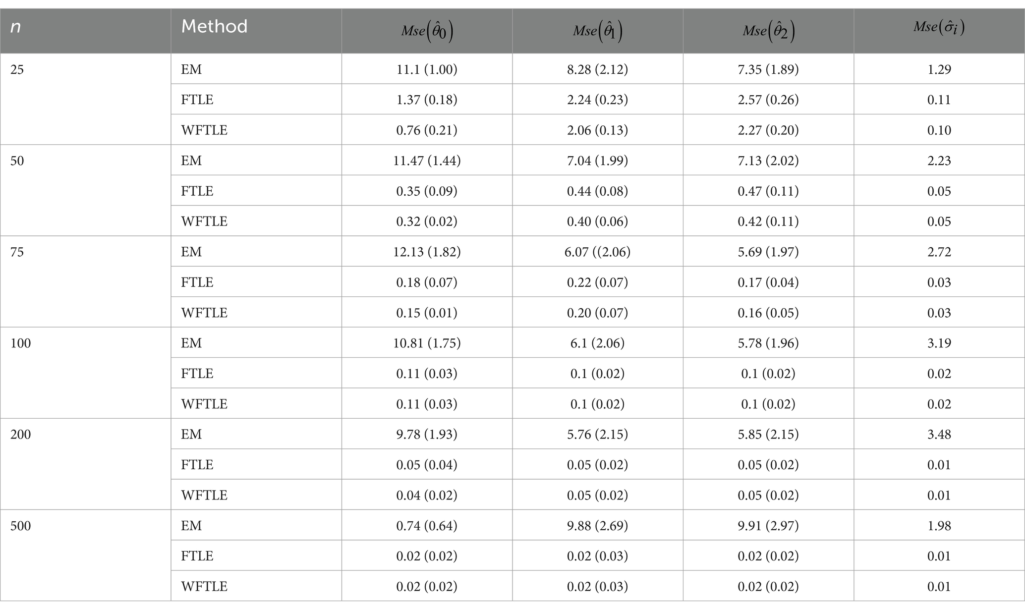
Table 3. $Mse\left({\widehat{\theta }}_i\right)$, $\mathit{Bias}\left({\widehat{\theta }}_i\right)$, and $Mse\left({\widehat{\sigma }}_i\right)$ for case III of the simulation study.

The market value of Iraq’s trade banks

To better demonstrate the robust performance of the WFTLE method compared to the FTLE and EM methods, we selected the market value data of Iraqi trade banks presented by Uraibi and Haraj (2022). From the original dataset, spanning 2011–2015, the Trading Rate and Earning Per Share (EPS) variables were selected out of nine financial ratios affecting market value. First, the regression model was fitted using the EM method, and the plotted residuals are shown in Figure 1.

Figure 1

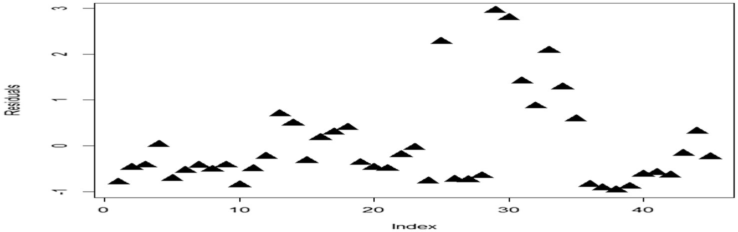
Figure 1. Residual plot of the regression model.

It is clear that there is more than one pattern in the residuals, each potentially representing a random distribution. This indicates a heterogeneity problem, leading to a mixture in the random distribution of residuals. Figure 2 further illustrates that the normalized EPS and trading rate ratios contain outliers (leverage points), as some data points lie far from the main cluster, suggesting heterogeneity. The performance of the WFTLE method proved superior to both the EM and FTLE methods, as evidenced by the market value data from the Iraq stock market presented in Table 4. The mean squared errors (MSE) and mean absolute errors (MAE) for WFTLE were 0.053 and 0.865, respectively, both of which are lower than the MSE and MAE of the other methods.

Figure 2

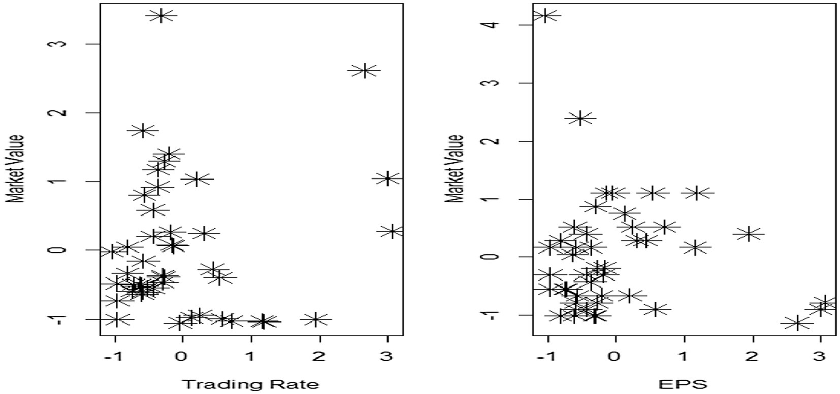
Figure 2. Scatter plot of trading rate and EPS.

Table 4

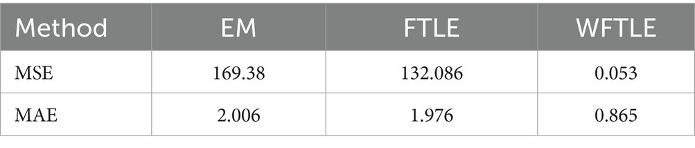
Table 4. The mean squared of errors (MSE) and mean absolute errors (MAE) of market value data.

Conclusion

The primary focus of this study is to improve the performance of the FTLE method in the presence of leverage points in mixture regression data. From the results presented in Tables 2–4, it can be concluded that the EM method is the most suitable choice where there are no outliers or leverage points. However, the EM method is highly susceptible to outliers and leverage points, as demonstrated by the variation in its results between Tables 2, 3. In contrast, the WFTLE method, especially for small sample sizes without trimming, demonstrates superior performance, even when outliers are present, as shown in Table 2. It also outperforms other methods when applied to real data. Trimming leverage points in small samples is not advisable, as it reduces the degrees of freedom, thereby increasing the value of MSE. Instead of discarding rows with leverage points by assigning zero weight, the WFTLE method assigns lower weights to those rows, preserving the degrees of freedom. This approach explains why the WFTLE method outperforms others in small sample sizes. Additionally, it is resistant to both outliers and leverage points, with both methods performing similarly in large sample sizes. The WFTLE method excels in small samples, though its performance may converge with FTLE when the number of observations reaches 100.

Data availability statement

The data analyzed in this study is subject to the following licenses/restrictions: no any restrictions that apply to the dataset. Requests to access these datasets should be directed to hssn.sami1@gmail.com.

Author contributions

HU: Project administration, Software, Supervision, Writing – review & editing. MW: Conceptualization, Data curation, Investigation, Methodology, Resources, Validation, Visualization, Writing – original draft.

Funding

The author(s) declare that no financial support was received for the research, authorship, and/or publication of this article.

Conflict of interest

The authors declare that the research was conducted in the absence of any commercial or financial relationships that could be construed as a potential conflict of interest.

Publisher’s note

All claims expressed in this article are solely those of the authors and do not necessarily represent those of their affiliated organizations, or those of the publisher, the editors and the reviewers. Any product that may be evaluated in this article, or claim that may be made by its manufacturer, is not guaranteed or endorsed by the publisher.

References

1. Quandt, RE . A New Approach to Estimating Switching Regressions. J Am Stat Assoc. (1972) 67:306–10. doi: 10.1080/01621459.1972.10482378

PubMed Abstract | Crossref Full Text | Google Scholar

2. Quandt, RE, and Ramsey, JB. Estimating mixtures of normal distributions and switching regressions. J Am Stat Assoc. (1978) 73:730–8. doi: 10.1080/01621459.1978.10480085

Crossref Full Text | Google Scholar

3. Huber, PJ . Robust statistics. New York: Wiley (1981).

Google Scholar

4. Rousseeuw, PJ, and Leroy, AM. Robust regression and outier detection. New York: Wiley (1987).

Google Scholar

5. Neykov, N, Filzmoser, P, Dimova, R, and Neytchev, P. Robust fitting of mixtures using the trimmed likelihood estimator. Comput Stat Data Anal. (2007) 52:299–308. doi: 10.1016/j.csda.2006.12.024

Crossref Full Text | Google Scholar

6. Dempster, AP, Laird, NM, and Rubin, DB. Maximum likelihood from incomplete data via theEMAlgorithm. J R Stat Soc Series B Stat Methodol. (1977) 39:1–22. doi: 10.1111/j.2517-6161.1977.tb01600.x

Crossref Full Text | Google Scholar

7. Peel, D, and McLachlan, GJ. Robust mixture modelling using the t distribution. Stat Comput. (2000) 10:339–48. doi: 10.1023/A:1008981510081

Crossref Full Text | Google Scholar

8. Hennig, C . Clusters, outliers, and regression: fixed point clusters. J Multivar Anal. (2003) 86:183–212. doi: 10.1016/S0047-259X(02)00020-9

PubMed Abstract | Crossref Full Text | Google Scholar

9. Markatou, M . Mixture models, robustness, and the weighted likelihood methodology. Biometrics. (2000) 56:483–6. doi: 10.1111/j.0006-341X.2000.00483.x

PubMed Abstract | Crossref Full Text | Google Scholar

10. Shen, R, Ghosh, D, and Chinnaiyan, AM. Prognostic meta-signature of breast cancer developed by two-stage mixture modeling of microarray data. BMC Genomics. (2004) 5:1–16. doi: 10.1186/1471-2164-5-94

Crossref Full Text | Google Scholar

11. Hadi, AS, and Luceño, A. Maximum trimmed likelihood estimators: a unified approach, examples, and algorithms. Comput Stat Data Anal. (1997) 25:251–72. doi: 10.1016/S0167-9473(97)00011-X

Crossref Full Text | Google Scholar

12. Vandev, DL, and Neykov, NM. About regression estimators with high breakdown point. Stat J Theor Appl Stat. (1998) 32:111–29. doi: 10.1080/02331889808802657

PubMed Abstract | Crossref Full Text | Google Scholar

13. Müller, CH, and Neykov, N. Breakdown points of trimmed likelihood estimators and related estimators in generalized linear models. J Stat Plan Inference. (2003) 116:503–19. doi: 10.1016/S0378-3758(02)00265-3

Crossref Full Text | Google Scholar

14. Rousseeuw, PJ, and Driessen, KV. A fast algorithm for the minimum covariance determinant estimator. Technometrics. (1999) 41:212–23. doi: 10.1080/00401706.1999.10485670

PubMed Abstract | Crossref Full Text | Google Scholar

15. García-Escudero, LA, Gordaliza, A, Matrán, C, and Mayo-Iscar, A. Avoiding spurious local maximizers in mixture modeling. Stat Comput. (2015) 25:619–33. doi: 10.1007/s11222-014-9455-3

Crossref Full Text | Google Scholar

16. Uraibi, HS . Weighted Lasso Subsampling for HighDimensional Regression. Electron J Appl Stat Anal. (2019) 12:69–84. doi: 10.1285/i20705948v12n1p69

Crossref Full Text | Google Scholar

17. Olive, D. J., and Hawkins, D. M. (2010), Robust multivariate location and dispersion. Preprint. Available at: https://lagrange.math.siu.edu/Olive/pphbmld.pdf

Google Scholar

18. Uraibi, HS, and Haraj, SAA. (2022). Group diagnostic measures of different types of outliers in multiple linear regression model. Mal. J. Fund. Appl. Sci. 41:23–33.

Google Scholar