Dynamic ensemble-based machine learning models for predicting pest populations

Early prediction of pest occurrences can enhance crop production, reduce input costs, and minimize environmental damage. Advances in machine learning algorithms facilitate the development of efficient pest alert systems. Furthermore, ensemble algorithms help in the utilization of several models rather than being dependent on a single model. This study introduces a dynamic ensemble model with absolute log error (ALE) and logistic error functions using four machine learning models—artificial neural networks (ANNs), support vector regression (SVR), k-nearest neighbors (kNN), and random forests (RF). Various abiotic factors such as minimum and maximum temperature, rainfall, and morning and evening relative humidity were incorporated into the model as exogenous variables. The proposed algorithms were compared with fixed-weighted and unweighted ensemble methods, and candidate machine learning models, using the pest population data for yellow stem borer (YSB) from two regions of India. Error metrics include the root mean square log error (RMSLE), root relative square error (RRSE), and median absolute error (MDAE), along with the Technique for Order Preference by Similarity to Ideal Solution (TOPSIS) algorithm. This study concluded that the proposed dynamic ensemble algorithm demonstrated better predictive accuracy in forecasting YSB infestation in rice crops.

1 Introduction

Agricultural pests in India pose a complex and significant threat to the country’s vital agricultural sector, which is the backbone of its economy and food supply. Improved crop production can be achieved by safeguarding crops from pests and increasing public awareness about the damage that pests can cause (1). Pests can cause extensive harm to crops, transmit dangerous plant diseases, and undermine crop productivity. In addition, temperature alterations impact the growth rates of various insect species. As global temperatures rise, agricultural losses due to insect pests are expected to increase by 10 to 25% for each degree of warming (2). Farmers have traditionally relied on pesticides and chemical treatments to get rid of pests. However, the widespread use of chemical pesticides also raises environmental and health concerns (3). Effectively addressing these agricultural pest challenges in India necessitates a comprehensive strategy that includes integrated pest management, sustainable farming practices, and increased investment in research and education, all of which are crucial for safeguarding crops and ensuring food security for the country’s ever-growing population. As agricultural practices shift toward advanced pest management, there is a growing need for innovative tools to reduce the uncertainties involved in estimating the levels of insect pest infestations in crop fields (4). To effectively address this challenge, integrated pest management strategies are essential. Regular monitoring, early detection, and appropriate control measures are crucial to minimize the damage caused by pests and ensure healthy, productive crop production.

Forecasting pest populations holds significant importance in agriculture and pest management for various compelling reasons. Early detection of potential pest outbreaks allows for proactive measures to safeguard crops, ultimately preventing substantial economic losses and ensuring a consistent food supply. In addition, it promotes sustainable agricultural practices by reducing reliance on chemical pesticides through accurate forecasting. This approach encourages the use of eco-friendly practices such as biological control and integrated pest management, which are beneficial to soil health and the overall ecosystem. Pest population forecasting serves as an indispensable tool for regulatory agencies and policymakers. It facilitates efficient resource allocation, enables quick responses to emerging pest threats, and aids in the development of policies and regulations that ensure agricultural productivity and food security.

2 Related work

Many researchers have proposed models for predicting pest populations and have compared them with other popular forecasting models. Li et al. (5) proposed a forecasting model for the vegetable pest flea beetle using the maximum likelihood algorithm. To develop effective pest management strategies for specific agricultural ecosystems, it is essential to gather information on the abundance and distribution of pests in relation to weather conditions (6). Arya et al. (7) used the autoregressive integrated moving average with exogenous variables (ARIMAX) model to predict pest populations using weather covariates in India. Paul et al. (8) applied statistical models to predict sterility mosaic disease in pigeon pea in Gujarat, India. Liu et al. (9) developed a monitoring and forecasting system for pest control based on a deep learning algorithm. Anwar et al. (1) developed a mathematical model to promote farmer awareness in crop pest management. Neta et al. (10) developed a temperature-dependent population dynamics model for the global insect pest Bemisia tabaci and verified its accuracy under field conditions.

Some recent studies have incorporated machine learning (ML) techniques to predict pest populations. Lankin-Vega et al. (11) proposed an ensemble model using artificial neural networks (ANNs) to predict the population of Rhopalosiphum padi (L.). Yan et al. (12) employed multiple regression (MR) and ANN modeling approaches to predict pest risks in crops. Paul et al. (13) predicted early blight severity in tomatoes using machine learning techniques. Skawsang et al. (14) applied ANN, random forests (RF), and MR analyses to predict the brown planthopper population using abiotic factors and host-plant phenology during the dry farming season from 2006 to 2016 in the Central Plains of Thailand. Paul et al. (15) developed an ML-based hybrid model for forecasting sterility mosaic disease in pigeon pea. Marković et al. (16) proposed an ML model to forecast the daily appearance of insects during a season, considering abiotic factors such as air temperature and relative humidity. Ibrahim et al. (17) applied a fuzzy neural network (FNN) model to predict the population of fruit flies in avocado crops. Paul et al. (18) developed a wavelet-based ML model for predicting the occurrence of spiders in pigeon pea. Sidumo et al. (19) suggested that the support vector machine (SVM) performs better than other machine learning models, such as RF, k-nearest neighbors (kNN), and ANN, in reducing over dispersion in count data. Predictions from ensemble methods, which are generated by combining multiple models, have gained popularity as they tend to provide more efficient forecasts compared to individual models. Galicia et al. (20) proposed ensemble learning for predicting time-series data and investigated two strategies for updating the weights: dynamic and static ensembles. The dynamic ensemble emerged as the better-performing model. Sharma et al. (21) proposed a bagging-based ensemble model for forecasting the number of incidences of disease based on past records. Abdelhamid and Alotaibi (22) proposed a two-level ensemble model, where the first level includes RF, support vector regression (SVR), and light gradient boosting algorithms, and the second level is based on the elastic net regression model. Du et al. (23) proposed a dynamic ensemble model based on Bayesian optimization, which provides a forecast combination for a time series with time-varying underlying patterns. Gangula et al. (24) implemented ensemble ML techniques within hybrid integrations to identify factors linked to the transmission of dengue fever, leading to enhanced performance outcomes. Sun et al. (25) and Jiang et al. (26) are some of the recent studies based on ensemble algorithms in different fields of time series forecasting. Dynamic ensemble methods involve the practice of allocating varying weights to candidate models within the ensemble. In such a scheme, the weights assigned to the base models can fluctuate either over time or according to specific conditions, overcoming the limitation of a fixed-weighted ensemble method. In fixed-weighted ensemble methods, the weights assigned to different candidate models are distinct but remain fixed.

The main objective of the present study is to utilize a time-dependent weighting scheme to ensemble forecasts obtained from machine learning models, such as ANN, SVR, kNN, and RF, using information available on exogenous weather factors for the prediction of pest populations. The weekly population of the yellow stem borer (YSB) pest, along with climatic factors affecting rice crops in Rajendranagar, Hyderabad, and Marteru, Andhra Pradesh, India, has been analyzed. The predictive accuracies of this approach were evaluated against candidate benchmark models, the unweighted ensemble method, and the weighted ensemble method, to forecast the data under consideration.

3 Methods

This study predicted pest populations based on historical data and abiotic factors. Pest population data are generally count data that exhibit over dispersion characteristics. In this section, popular machine learning models used as candidate models in the ensemble approach are briefly discussed.

3.1 Candidate model

3.1.1 Artificial neural network (ANN)

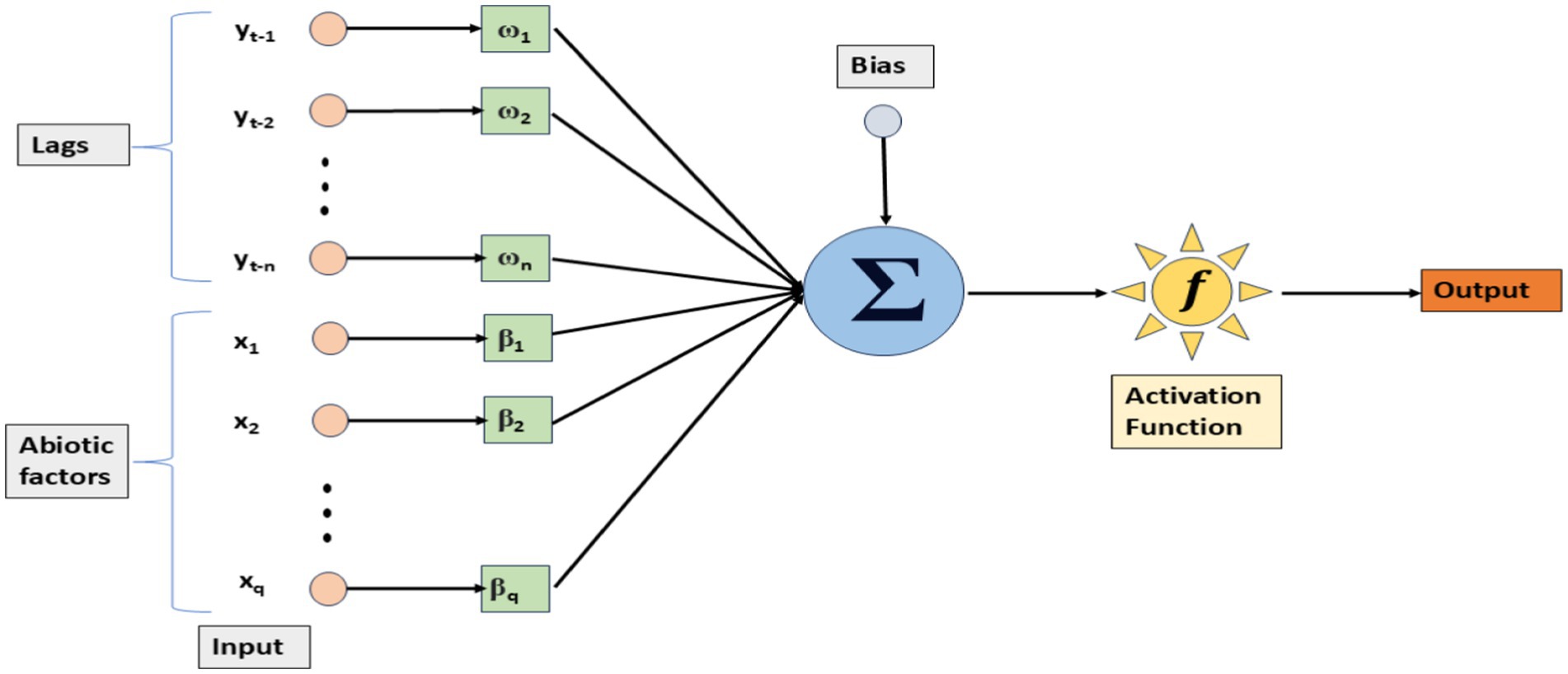
An artificial neural network (ANN) is a mathematical model inspired by the human brain, designed to tackle complex problems in scientific research and engineering applications. The fundamental building block of an ANN is the neuron, and these neurons are structured into three different layers: the input layer, the hidden layer, and the output layer. The input layer represents the input parameters, the output layer corresponds to the predicted outcomes, and the hidden layer serves as an artificial layer that captures non-linear relationships. In this study_, we considered an ANN with an exogenous variable model, i.e., the ANN-X model (Figure 1), which includes a time series sequence from y_t-1 to y_t-n, with n, the number of lags, and abiotic factors, such as maximum temperature (Tmax), minimum temperature (Tmin), relative humidity-morning (RHM), relative humidity-evening (RHE), and rainfall (RF), as inputs.

Figure 1

Figure 1. Architecture of the ANN-X model, with the lag value and abiotic factors as inputs.

To model a time series using an ANN with an exogenous variable, a non-linear function (f) is created, that operates on a sequence of values (y_t) from y_t-1 to y_t-n, where n is the number of lags and x₁, x₂, … x_q denote the abiotic factors.

$\begin{array}{ll}{y}_t=w_0+{\displaystyle \sum _{j=1}^h{w}_{j}f}\left(w_{0j}+{\displaystyle \sum _{i=1}^n{w}_{ij}{y}_{t-i}+}{\displaystyle \sum _{k=1}^q{g}_{kj}{x}_k}\right)+e_t& (1)\end{array}$

In Equation 1, w_ij, g_kj, and w_j represent the weights, while h, n, and e_t represent the number of hidden nodes, the number of input nodes, and the error term, respectively. The activation function for the hidden layers in an ANN model can take various forms, such as sigmoid, RLU, and tanh. The application of an ANN is well-known in disease and epidemic prediction. Niazkar and Niazkar (35) used an ANN for the prediction of the COVID-19 outbreak.

3.1.2 K-nearest neighbors (kNN)

The kNN algorithm is a non-parametric technique that retains all available data points and makes predictions for numerical targets by assessing similarity, often using distance metrics. In kNN regression, a basic implementation involves computing the mean of the numerical targets from the k nearest neighbors. Alternatively, another approach utilizes a weighted average based on the inverse distance of kNN. kNN regression applies distance functions such as Euclidean, Manhattan, and Minkowski. For example, de Oliveira Aparecido et al. (27) used kNN to predict the incidence of pests in Coffea arabica.

The kNN model is given in Equation 2:

$\begin{array}{ll}\mathit{Outpu}{t}_{kNN}=f\left(u\right)& (2)\end{array}$

where u contains exogenous variables (abiotic factors) and a sequence of a time series from y_t-1 to y_t-n, and n is the number of lags.

3.1.3 Support vector regression (SVR)

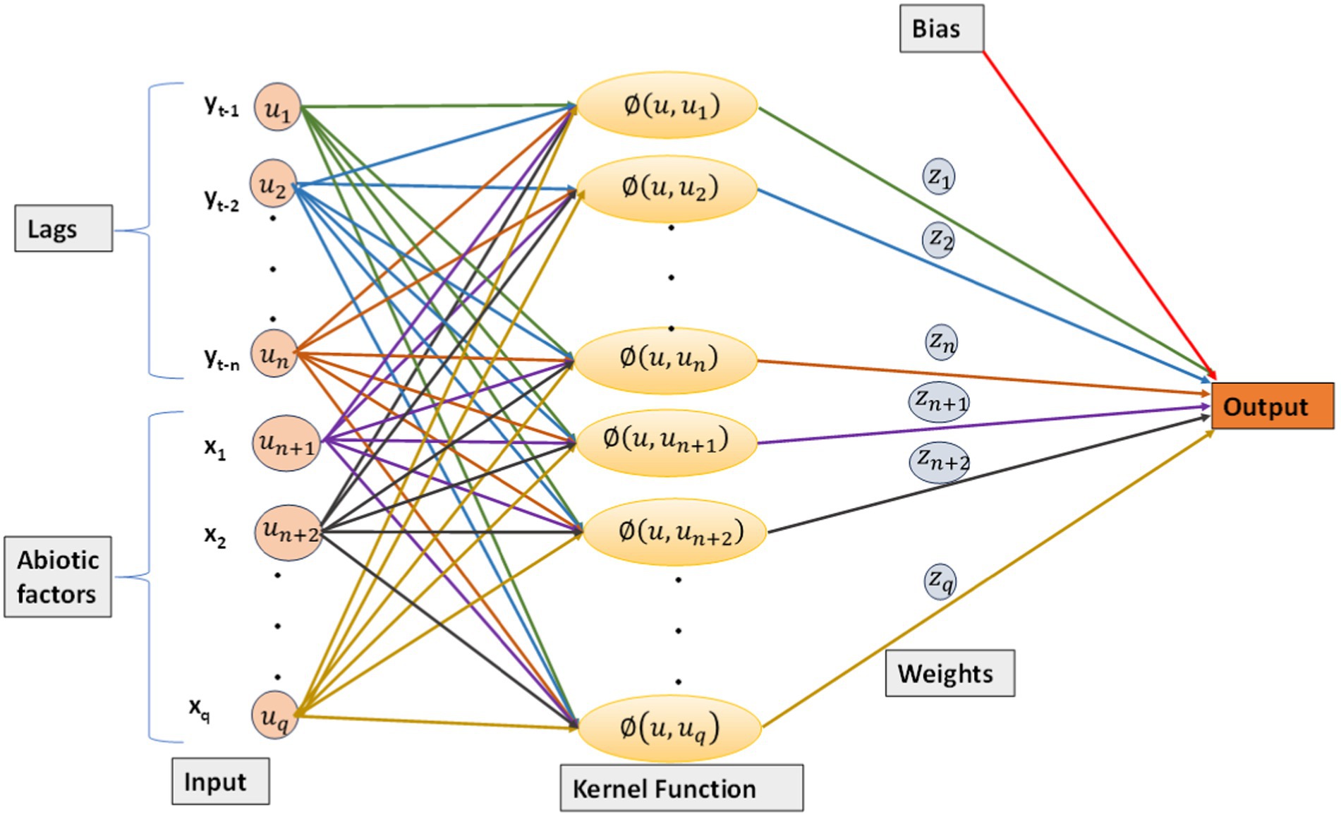
SVR can effectively address non-linear associations between input variables and the target variable by applying a kernel function to relocate the data into a higher-dimensional space. This feature enhances its suitability for regression tasks involving intricate relationships between input variables and the target variable.

The SVR-X model can be formulated as follows:

$\begin{array}{ll}f\left(u\right)=z\varnothing \left(u\right)+b& (3)\end{array}$

where u contains abiotic factors and a sequence of a time series from y_t-1 to y_t-n, and n is the number of lags. The estimated function of the dataset, i.e., $f\left(u\right)$ in Equation 3, is the output of the model. The process involves applying a kernel function $\varnothing \left(\cdot \right)$ to relocate non-linear data to a higher-dimensional feature space, treating this transformed data as if it were linear, and then computing a dot product with a weight vector, represented as ‘z.’ This dot product is combined with a bias term ‘b’ to produce the final estimation. Figure 2 shows the architecture of SVR-X with abiotic factors and lags as inputs.

Figure 2

Figure 2. Schematic diagram of SVR-X.

Thus, the SVR model can be formulated as follows:

$\begin{array}{ll}f\left(u,z\right)=f\left(u,\alpha ,{\alpha }^{\ast }\right)={\displaystyle \sum _i\left({\alpha }_i-{\alpha }_i^{\ast }\right)}\varnothing \left(u,u_i\right)+b& (4)\end{array}$

where,$\varnothing \left(\cdot \right)$ is the kernel function. The RBF kernel is the most commonly used kernel in SVR model building (28–30). The RBF kernel is presented in Equation 5.

$\begin{array}{ll}\varnothing \left(x,x_i\right)=exp\left(-\frac{{\left|\right|x-x_i\left|\right|}^2}{2{\sigma }^2}\right)& (5)\end{array}$

The hyper-parameters used in the model are tuned using the Lagrange method. The terms $a,a^{\ast }$ mentioned in Equation 4 denote the Lagrange multipliers and should satisfy the following equality: $a_j{a}_j^{\ast }=0$.

3.1.4 Random forests (RF)

RF (31) is an ensemble learning method based on decision trees. Since its introduction, it has become one of the most popular algorithms in machine learning. Its widespread adoption is attributed to its ability to perform well in diverse applications, even in high-dimensional settings. It is recognized for its computational efficiency and ease of tuning. In classification, a decision tree serves as a straightforward model, where internal nodes represent attribute tests, branches indicate test outcomes, and leaves contain class labels. Decision trees can also handle regression tasks when the target variable is continuous. RF employs a specific technique called bootstrap aggregation, or bagging, where each decision tree is trained on a randomly chosen subsample of the complete training dataset. Successful implementations can be found in various areas, including the prediction of time series data (32).

3.2 Ensemble methods for forecasting

Ensemble methods are a popular approach in forecasting, involving a combination of predictions from multiple individual models to improve the overall forecast accuracy and robustness. These methods leverage the idea that different models can capture different aspects of the underlying data patterns and, when combined, can provide more accurate and reliable forecasts. The predictions from multiple individual models are combined using weights.

The unweighted ensemble approach assigns equal weight to each candidate model. Here, suppose ${\stackrel{⌢}{y}}_1$, ${\stackrel{⌢}{y}}_2$, … ${\stackrel{⌢}{y}}_N$ are the forecasted values obtained from N number of models. Then, the forecast from the unweighted ensemble method (${\stackrel{⌢}{y}}_{uw}$) is given in Equation 6.

$\begin{array}{ll}{\stackrel{⌢}{y}}_{uw}=\frac{1}{N}\left({\displaystyle \sum _{i=1}^N{\stackrel{⌢}{y}}_i}\right)& (6)\end{array}$

In the weighted ensemble approach, the weights of the candidate models vary but can be determined using an optimization algorithm. Therefore, the forecast from the weighted ensemble method (${\stackrel{⌢}{y}}_{fw}$) is given in Equation 7.

$\begin{array}{ll}{\stackrel{⌢}{y}}_{fw}=\left({\displaystyle \sum _{i=1}^N{w}_i}{\stackrel{⌢}{y}}_i\right)& (7)\end{array}$

where w_i is the weight assigned to the ith candidate model such that ${\displaystyle \sum _{i=1}^N{w}_i}$= 1. The weights are optimized using population-based optimization algorithms, such as particle swarm optimization (PSO). Population-based optimization algorithms, such as PSO, offer the benefit of concurrently exploring a wide range of potential solutions, enhancing the chances of discovering the global optimum while preventing entrapment in local optima (33).

A dynamic weighting scheme in an ensemble method involves the practice of allocating varying weights to candidate models. These weight adjustments are made in response to model performance or other factors. In such a scheme, the weights assigned to the base models can fluctuate either over time or based on specific conditions.

3.2.1 Time-dependent dynamic ensemble model

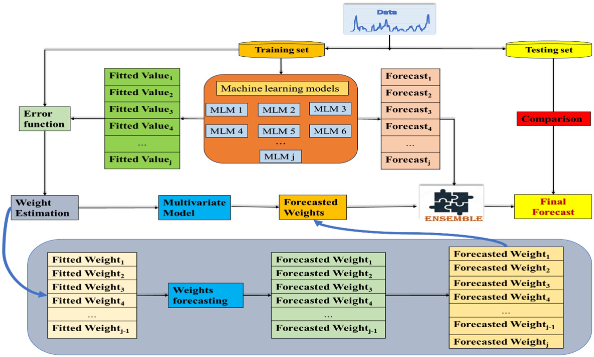
Deb and Deb (34) proposed the use of a time-dependent weighting scheme based on an error function for generating predictions using an ensemble approach. In this study, the forecasts obtained from the different machine learning techniques were ensembled using the time-dependent weighting scheme (Figure 3). One of the advantages of using a time-dependent dynamic weighting scheme is that the weights are adjusted at each point of time. Let ${\stackrel{⌢}{y}}_t^{\left(1\right)}$, ${\stackrel{⌢}{y}}_t^{\left(2\right)}$ … ${\stackrel{⌢}{y}}_t^{\left(j\right)}$ represent the values of the output obtained by model (1), model (2) … model (j), i.e., j candidate models at time t. As the dataset is divided into a training set (A) and a testing set (B), ${\stackrel{⌢}{y}}_t^{\left(1\right)}$, ${\stackrel{⌢}{y}}_t^{\left(2\right)}$ … ${\stackrel{⌢}{y}}_t^{\left(j\right)}$ are the fitted values of the j candidate models at time t, where t∊ A, and A represent the training set.

Figure 3

Figure 3. Flowchart of the time-dependent weighting scheme ensemble forecasting approach.

${\stackrel{⌢}{y}}_{t\prime }^{\left(1\right)}$, ${\stackrel{⌢}{y}}_{t\prime }^{\left(2\right)}$… ${\stackrel{⌢}{y}}_{t\prime }^{\left(j\right)}$ represent the predicted values from the j candidate models at time $t^{\prime }$, where ${\text{t}}^{\prime }$∊ B, and B represent the prediction set. $w_t^{\left(i\right)}$ is the forecasted weight obtained for the i^th candidate model at time $t$ such that ${\displaystyle \sum _{i=1}^j{w}_t^{\left(i\right)}}=1$.

The weighted ensemble approach to predict $y_{t\prime }$, ${\text{t}}^{\prime }$∊ B is given in Equation 8.

$\begin{array}{ll}{\stackrel{⌢}{y}}_{t\prime }={\displaystyle \sum _{i=1}^j{w}_{t\prime }^{\left(i\right)}}{\stackrel{⌢}{y}}_{t\prime }^{\left(i\right)}& (8)\end{array}$

The weights of the time-dependent weighting scheme are determined by

$\begin{array}{ll}{w}_t^{\left(i\right)}=\frac{\raisebox{1ex}{$1$}\!\left/ \!\raisebox{-1ex}{$E_t^{\left(i\right)}$}\right.}{\left({\displaystyle \sum _{i=1}^j\raisebox{1ex}{$1$}\!\left/ \!\raisebox{-1ex}{$E_t^{\left(i\right)}$}\right.}\right)}& (9)\end{array}$

In Equation 9, $E_t^{\left(i\right)}$ is the error obtained for the i^th model at time t, such that ${\displaystyle \sum _{i=1}^j{w}_t^{\left(i\right)}}=1$.

Therefore, at each point of time in the training set, the weights assigned to each method are determined based on an inverse relationship with the error function. The logistic error function and the absolute log error (ALE) function are used to obtain the weights.

The expression for the logistic error function is given in Equation 10.

$\begin{array}{ll}{E}_t^{\left(i\right)}=\frac{1}{\left(1+exp(-\mathit{abs}\left({\stackrel{⌢}{y}}_t^{\left(i\right)}-y_t\right)\right)}& (10)\end{array}$

The expression for the absolute log error function is given in Equation 11.

$\begin{array}{ll}{E}_t^{\left(i\right)}=\left|\log \left({\stackrel{⌢}{y}}_t^{\left(i\right)}+1\right)-\log \left(y_t+1\right)\right|& (11)\end{array}$

The matrix of the weights $W$ obtained for t ∊ A can be treated as a multivariate time series since the sum of all weights is equal to 1, which shows that the weight components are interdependent among each other.

$\mathrm{Where,}W=\left(w^{\left(1\right)}\mathrm{,}{w}^{\left(2\right)}\mathrm{,}\dots w^{\left(j\right)}\right)=\mathrm{\hspace{0.33em}}\mathrm{\hspace{0.33em}}\left[\begin{array}{ccc}\begin{array}{cc}{w}_1^{\left(1\right)}& w_1^{\left(2\right)}\\ w_2^{\left(1\right)}& w_2^{\left(2\right)}\end{array}& \cdots & \begin{array}{c}{w}_1^{\left(j\right)}\\ w_2^{\left(j\right)}\end{array}\\ ⋮& \ddots & ⋮\\ w_n^{\left(1\right)}\mathrm{\hspace{0.33em}}\mathrm{\hspace{0.33em}}{w}_n^{\left(2\right)}& \cdots & w_n^{\left(j\right)}\end{array}\right].$

A matrix with independent columns $W^{\ast }=\left(w^{\left(1\right)}\mathrm{,}{w}^{\left(2\right)}\mathrm{,}\dots w^{\left(j-1\right)}\right)\mathrm{\hspace{0.33em}}$is constructed from $W$ by deleting the column corresponding to the j^th model to obtain an estimate of the weight. For ${\text{t}}^{\prime }$∊ B, the weights are forecasted by fitting a vector autoregressive (VAR) model to the multivariate time series $W^{\ast }$. The forecasts of the weights obtained from the VAR model, corresponding to (j-1) number of models, are arranged in the matrix ${\stackrel{⌢}{W}}^{\ast }$ so that the ith column represents the forecasted weights corresponding to the ith candidate model. Thus, the weight matrix ${\stackrel{⌢}{W}}^{\ast }$ for the h-step ahead forecast obtained from the VAR model is defined as ${\stackrel{⌢}{W}}^{\ast }=\left({\stackrel{⌢}{w}}^{\left(1\right)}\mathrm{,}{\stackrel{⌢}{w}}^{\left(2\right)}\mathrm{,}\dots {\stackrel{⌢}{w}}^{\left(\mathrm{j}-1\right)}\right)=\mathrm{\hspace{0.33em}}\mathrm{\hspace{0.33em}}\left[\begin{array}{ccc}\begin{array}{cc}{\stackrel{⌢}{w}}_{\mathrm{n}+1}^{\left(1\right)}& {\stackrel{⌢}{w}}_{\mathrm{n}+1}^{\left(2\right)}\\ {\stackrel{⌢}{w}}_{\mathrm{n}+2}^{\left(1\right)}& {\stackrel{⌢}{w}}_{\mathrm{n}+2}^{\left(2\right)}\end{array}& \cdots & \begin{array}{c}{\stackrel{⌢}{w}}_{\mathrm{n}+1}^{\left(j-1\right)}\\ {\stackrel{⌢}{w}}_{\mathrm{n}+2}^{\left(j\right)}\end{array}\\ ⋮& \ddots & ⋮\\ \begin{array}{cc}{\stackrel{⌢}{w}}_{n+h}^{\left(1\right)}& w_{n+h}^{\left(2\right)}\end{array}& \cdots & {\stackrel{⌢}{w}}_{n+h}^{\left(j\right)}\end{array}\right]$

The column of the forecasted weights corresponding to the j^th model is defined as ${\stackrel{⌢}{w}}^{\left(j\right)}=\left\{1-{\displaystyle \sum _{i=1}^{j-1}{\stackrel{⌢}{w}}^{\left(i\right)}}\right\}$. The weight matrix $\stackrel{⌢}{W}$, containing the weights corresponding to all j candidate models, is obtained by augmenting ${\stackrel{⌢}{W}}^{\ast }$ with ${\stackrel{⌢}{w}}^{\left(j\right)}$ as $\stackrel{⌢}{W}={\left({\stackrel{⌢}{w}}^{\left(1\right)}\mathrm{,}{\stackrel{⌢}{w}}^{\left(2\right)}\mathrm{,}\dots {\stackrel{⌢}{w}}^{\left(j-1\right)}\mathrm{,}{\stackrel{⌢}{w}}^{\left(j\right)}\right)}^{\prime }$. The kth row of the matrix $\stackrel{⌢}{W}$ contains the forecasted weights corresponding to the k^th candidate model.

Consider $\stackrel{⌢}{Y}=\left({\stackrel{⌢}{y}}^{\left(1\right)}\mathrm{,}{\stackrel{⌢}{y}}^{\left(2\right)}\mathrm{,}\dots {\stackrel{⌢}{y}}^{\left(j\right)}\right)$, where ${\stackrel{⌢}{y}}^{\left(i\right)}$ is the vector of the forecasted value obtained from the ith candidate model. Then, the dynamic weighted ensemble forecast ${\stackrel{⌢}{y}}_{dw}$ is given by Equation 12, which is obtained from the multiplication of the matrix $\stackrel{⌢}{W}$ and $\stackrel{⌢}{Y}$. Therefore, the dynamic forecast can be computed using Equation 12.

$\begin{array}{ll}{\stackrel{⌢}{y}}_{dw}=\stackrel{⌢}{W}\ast \stackrel{⌢}{Y}& (12)\end{array}$

3.3 Performance measures

Accuracy metrics, such as the root mean square log error (RMSLE), root relative square error (RRSE), and median absolute error (MDAE), were used to compare the performance of the proposed dynamic ensemble model with the candidate models, the unweighted ensemble model, and the fixed-weighted ensemble model. The values of the RMSLE, RRSE, and MDAE for the ith model are given by the expressions mentioned in Equations 13–15, respectively.

Root Mean Squared Logarithmic Error (RMSLE)

$\begin{array}{ll}RMSLE=\sqrt{\frac{1}{N}{\displaystyle \sum _{t=1}^N{\left(\log \left({\stackrel{⌢}{y}}_t^{\left(i\right)}+1\right)-\log \left(y_t+1\right)\right)}^2}}& (13)\end{array}$

Root Relative Square Error (RRSE).

$\begin{array}{ll}RRSE=\sqrt{{{\displaystyle \sum }}_{t=1}^N{\left(y_t-{\stackrel{⌢}{y}}_t^{\left(i\right)}\right)}^2/{{\displaystyle \sum }}_{t=1}^N{\left(y_t-\overline{y}\right)}^2}& (14)\end{array}$

Median Absolute Error (MDAE).

$\begin{array}{ll}MDAE=median\left(\left|y_1-{\stackrel{⌢}{y}}_1^{\left(i\right)}\right|\mathrm{,}\left|y_2-{\stackrel{⌢}{y}}_2^{\left(i\right)}\right|\mathrm{,}\dots \left|y_N-{\stackrel{⌢}{y}}_N^{\left(i\right)}\right|\right)& (15)\end{array}$

where $y_t$ is the actual value at time t, and ${\stackrel{⌢}{y}}_t^{\left(i\right)}$ is the forecasted value from the ith model at time t. $\overline{y}$ is the mean of the actual value, and N is the total number of observations.

4 Results and discussion

4.1 Data description and preprocessing

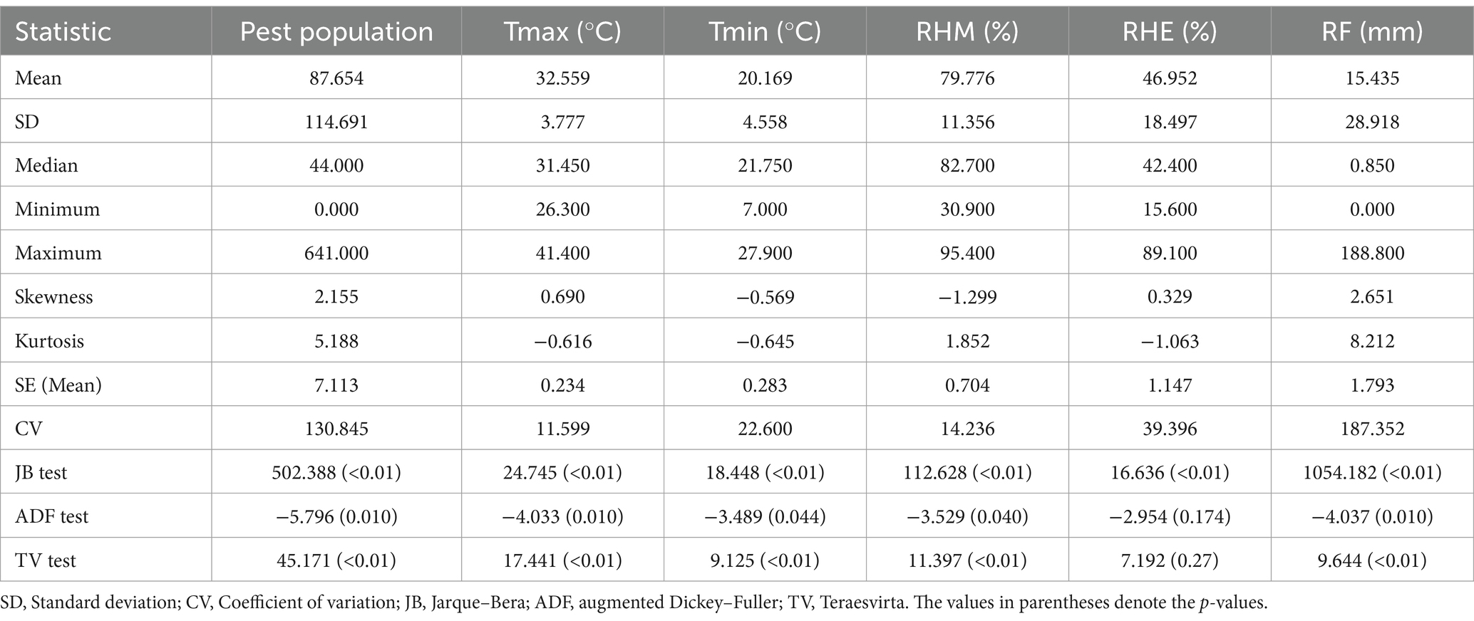
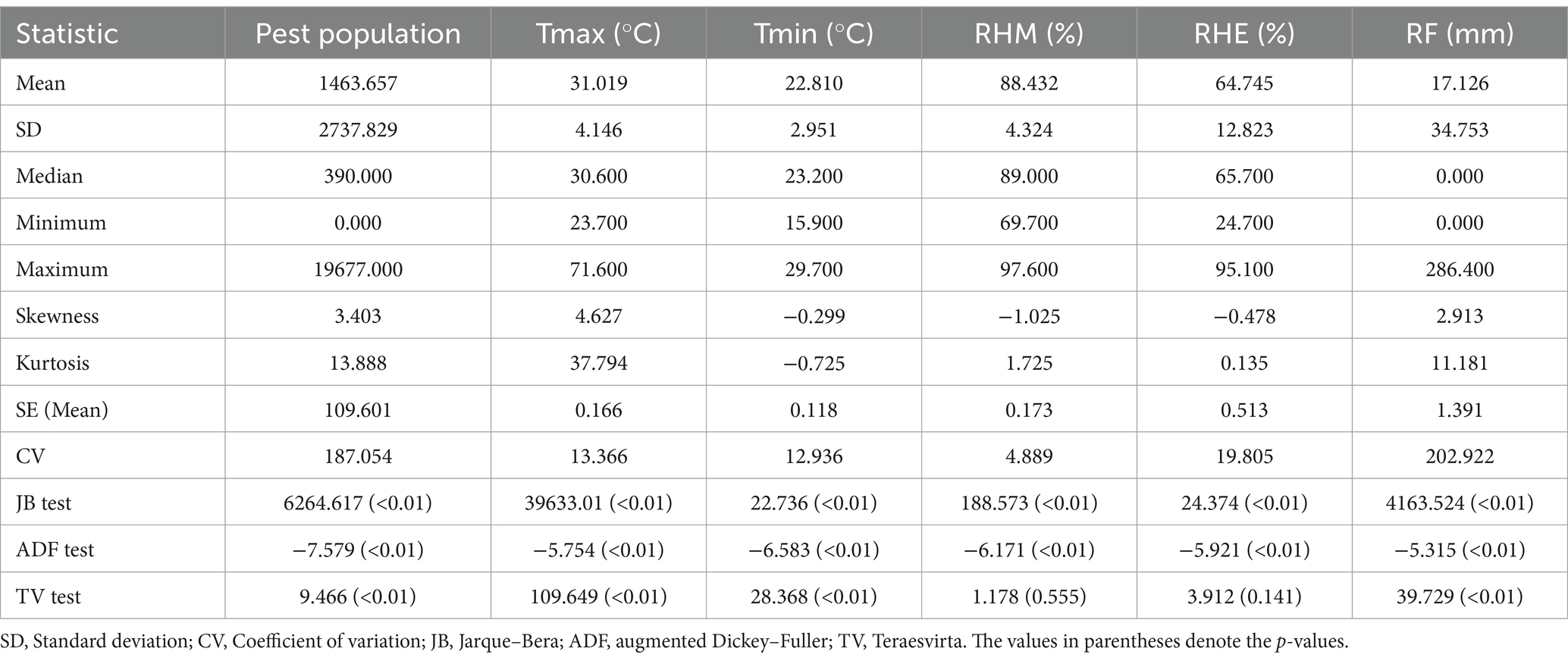
The weekly population (Y) of the yellow stem borer (YSB), Scirpophaga incertulas, in rice, along with climatic factors, including maximum temperature (Tmax), minimum temperature (Tmin), relative humidity-morning (RHM), relative humidity-evening (RHE), and rainfall (RF) in Rajendranagar, Hyderabad, and Marteru, Andhra Pradesh, India, were obtained from the Croppest DSS portal of the Central Research Institute for Dryland Agriculture, India.¹ The data ranged from 2007 to 2011 for Rajendranagar and from 2000 to 2011 for Marteru. Each year comprised 52 standard meteorological weeks (SMWs). The rationale behind the selection of the YSB pest was that it is a major pest of rice and has a widespread, devastating impact on the income of rice farmers. This pest affects rice plants at multiple growth stages, particularly during the vegetative and reproductive phases, causing significant yield losses. The descriptive statistics, kernel density, and box plots of the data under consideration are presented in Tables 1, 2 and Figure 4, respectively.

Table 1

Table 1. Descriptive statistics of the pest population and climatic data from Rajendranagar.

Table 2

Table 2. Descriptive statistics of the pest population and climatic data from Marteru.

Figure 4

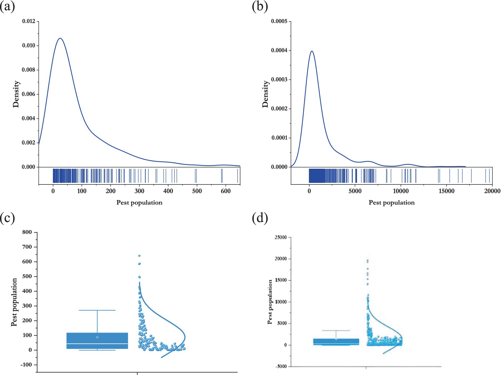
Figure 4. Kernel density (A) Rajendranagar; (B): Marteru and box plot (C): Rajendranagar; (D) Marteru of the pest populations.

From Tables 1, 2, it can be observed that the mean of the pest populations exceeded the variance, indicating a characteristic of a negative binomial distribution. Furthermore, the average pest population in Marteru was higher than that in Rajendranagar. Both pest datasets were positively skewed and leptokurtic in nature. Notably, the coefficient of variation (CV) for both datasets exceeded 100%, signifying a high degree of variation. Marteru data exhibited greater variability compared to the Rajendranagar data. The Jarque–Bera test was implemented to check the normality of the datasets, and it was found that all the data series were non-normal in nature. The stationarity of the data was examined using the augmented Dickey–Fuller (ADF) test. The ADF test inferred that, except for the RHE from Rajendranagar, all the data series followed the stationarity assumption. The results of the Teraesvirta neural network test suggested that, except for the RHM from Marteru, all the data series were non-linear. The insights from the descriptive statistics are further substantiated by Figure 2.

The Spearman’s correlation of the pest populations with all the abiotic factors was computed and is presented in Table 3. Figure 5 represents the cross-correlation analysis of both regions. The correlation at lag k estimates the relationship between the pest population at time t + k and the climatic factors at time t. The correlation in Figure 5 clearly shows that the climatic factors had a significant effect on the incidence of the pest populations at different lags. For the Rajendranagar region, Tmax, Tmin, RHM, and RHE had significant leading and lagging effects, and RF had significant lagging effects on the pest population. For the Marteru region, Tmax, Tmin, RHM, RHE, and RF had significant leading and lagging effects on the pest population.

Table 3

Table 3. Correlation value between the pest population and abiotic factors.

Figure 5

Figure 5. Cross-correlation analysis (A) Rajendranagar; (B) Marteru.

Table 3 shows the significant association between the pest populations and abiotic factors. The pest populations had a positive correlation with maximum and minimum temperature and a negative correlation with RHM, RHE, and rainfall.

4.2 Implementation of machine learning models

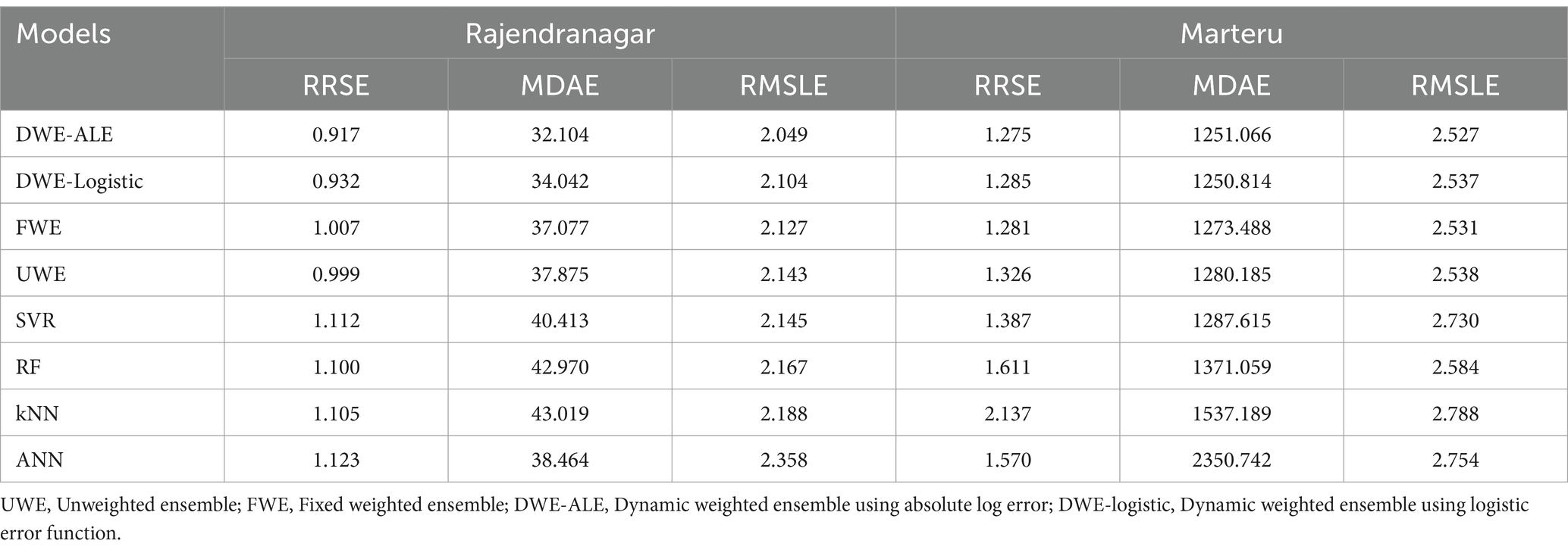
The weekly pest population data were divided into training and test sets in an 80:20 ratio. For Marteru, the training set comprised the first 499 observations for model building, leaving the remaining 126 observations for model validation. Similarly, for Rajendranagar, the training set included the initial 260 observations for model building, while the remaining 52 observations were reserved for model validation. Four machine learning models—ANN, SVR, kNN, and RF—were employed to model the weekly pest population count, utilizing information on abiotic factors. The 12 SMWs were considered the number of lags. Hyperparameter optimization is a crucial step in building machine learning models. The grid search method was used to optimize the hyperparameters systematically. This algorithm explores a predefined range of hyperparameter values for a given model. The hyperparameter set that yielded the highest performance was selected and is presented in Table 4.

Table 4

Table 4. Hyperparameter specification for the machine learning models.

In the class of ensemble models, unweighted, fixed-weighted, and dynamic-weighted ensemble models were implemented, as outlined in the methodology. In the fixed-weighted ensemble methods, the weights were optimized using population-based optimization algorithms, such as PSO, and the results are detailed in Table 5. The values of the weights for the fixed-weighted ensemble methods showed that, for the Rajendranagar region, the highest weightage was given to the ANN (0.441), whereas the lowest weightage was given to the RF (0.111). For the Marteru region, the highest weightage was given to the kNN (0.509), whereas the lowest weightage was given to the ANN (0.089). These variations in the performance of the models for both regions suggest that no single model can perform better in all the cases. As for the optimized weights, the ANN was given more importance in the Rajendranagar region but less weightage in the Marteru region among all the candidate models. These differences also support the use of ensemble models for prediction rather than relying on a single model. Performance measures based on the testing data were calculated and are presented in Table 6.

Table 5

Table 5. Optimized weight obtained for the ML model in the fixed-weighted ensemble model.

Table 6

Table 6. Performance measures of the implemented models.

According to Table 6, in the Rajendranagar region, the dynamic-weighted ensemble model outperformed all other models across all three performance measures. Within the dynamic ensemble models, the model utilizing the error function RRSE exhibited superior performance. Both the fixed-effect and weighted ensemble models outperformed the other machine-learning models. Between the fixed-effect and weighted ensemble models, except for the RRSE, the weighted ensemble models proved to be superior based on the other two measures.

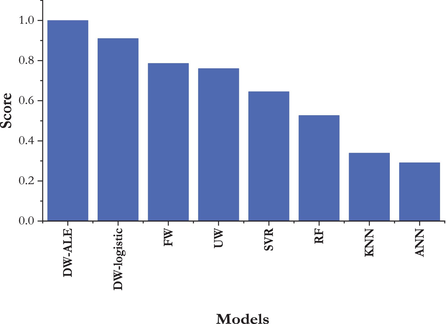
For the Marteru region, the DWE-ALE outperformed the others based on the RRSE and RMSLE, while the DWE-logistics excelled in terms of MDAE. However, the fixed-weighted ensemble models performed better than the DWE-logistics model based on the RRSE and RMSLE. Although the proposed model performed better than the other models in the data having extreme variation, the Technique for Order Preference by Similarity to Ideal Solution (TOPSIS) was employed to identify the best model among all implemented models across both datasets and three measures. The rankings and TOPSIS scores are presented in Figure 6.

Figure 6

Figure 6. Combined TOPSIS scores of all implemented models.

Figure 6 clearly illustrates that the dynamic ensemble model outperformed the other models, and among the dynamic models, the DWE-ALE model exhibited superior performance. Following the dynamic models, the fixed-effect ensemble model performed better than the unweighted ensemble model. Among the machine learning models, the SVR model, followed by the RF model, demonstrated high prediction accuracy, while the ANN model ranked lower in the TOPSIS score. The actual and fitted values of the best model, the DWE-ALE, are depicted in Figure 7.

Figure 7

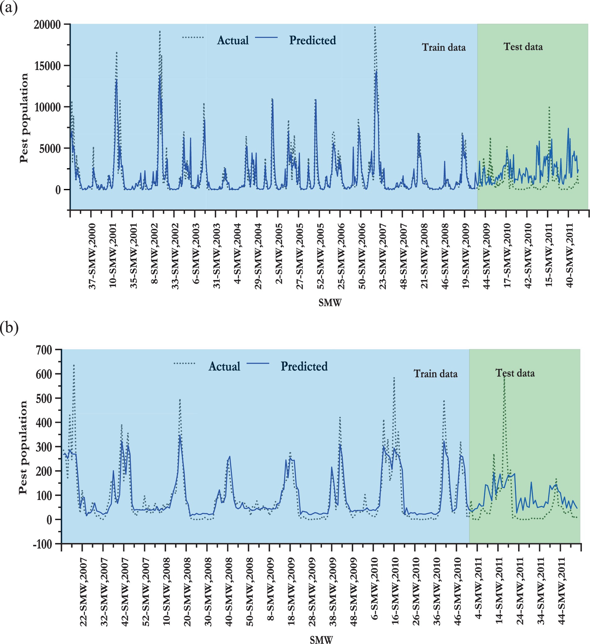
Figure 7. Plot of the actual and predicted values of the best-fitted models for (A) Rajendranagar and (B) Marteru.

5 Conclusion

The development of a pest forewarning system remains a significant challenge for farmers and policymakers. This study provides a detailed overview of an ensemble model with a time-dependent weighting scheme and introduces a time-varying dynamic ensemble approach with ALE and logistic error functions using four candidate models, namely ANN, SVR, kNN, and RF, for pest infestation modeling. Abiotic factors, such as minimum and maximum temperature, rainfall, and morning and evening relative humidity, were also considered in the model. This study found that the YSB population of rice had a positive correlation with maximum and minimum temperature and a negative correlation with RHM, RHE, and rainfall. The proposed algorithms were empirically compared with fixed-weighted and unweighted ensemble methods, as well as all four candidate models, using three performance metrics and the TOPSIS algorithm. The dynamic ensemble algorithm demonstrated higher predictive accuracy in predicting the YSB in rice crops in both regions. These algorithms showed promise for implementation in pest risk warning systems, aligning well with observed trends in actual field data for pests. Consequently, farmers can proactively manage pests using the predictive insights provided by our proposed model. This study on dynamic ensemble models paves the way for a new era of hybrid models. In future studies, this model can be further examined using other pest populations from various crops. This model can also be improved by incorporating other error functions and advanced multivariate learning models for weight forecasting.

Data availability statement

Publicly available datasets were analyzed in this study. This data can be found at: http://www.icar-crida.res.in:8080/naip/AccessData.jsp.

Author contributions

AKS: Data curation, Formal analysis, Investigation, Methodology, Writing – original draft. MY: Investigation, Methodology, Software, Validation, Writing – review & editing. RP: Conceptualization, Supervision, Visualization, Writing – review & editing. AP: Conceptualization, Supervision, Validation, Writing – review & editing. AS: Data curation, Formal analysis, Writing – review & editing.

Funding

The author(s) declare that no financial support was received for the research, authorship, and/or publication of this article.

Conflict of interest

The authors declare that the research was conducted in the absence of any commercial or financial relationships that could be construed as a potential conflict of interest.

Publisher’s note

All claims expressed in this article are solely those of the authors and do not necessarily represent those of their affiliated organizations, or those of the publisher, the editors and the reviewers. Any product that may be evaluated in this article, or claim that may be made by its manufacturer, is not guaranteed or endorsed by the publisher.

Footnotes

1. ^http://www.icar-crida.res.in:8080/naip/index.jsp

References

1. Anwar, N, Ahmad, I, Kiani, AK, Shoaib, M, and MAZ, R. Numerical treatment for mathematical model of farming awareness in crop pest management. Front Appl Math Stat. (2023) 9:1208774. doi: 10.3389/fams.2023.1208774

Crossref Full Text | Google Scholar

2. Deutsch, CA, Tewksbury, JJ, Tigchelaar, M, Battisti, DS, Merrill, SC, Huey, RB, et al. Increase in crop losses to insect pests in a warming climate. Science. (2018) 361:916–9. doi: 10.1126/science.aat3466

PubMed Abstract | Crossref Full Text | Google Scholar

3. Rani, L, Thapa, K, Kanojia, N, Sharma, N, Singh, S, Grewal, AS, et al. An extensive review on the consequences of chemical pesticides on human health and environment. J Clean Prod. (2021) 283:124657. doi: 10.1016/J.JCLEPRO.2020.124657

Crossref Full Text | Google Scholar

4. Olatinwo, R, and Hoogenboom, G. Weather-based Pest forecasting for efficient crop protection In: DP Abrol, editor. Integrated Pest management: Current concepts and ecological perspective. London: Academic Press (2014). 59–78.

Google Scholar

5. Li, T, Yang, J, and Chen, Z. The early warning and prediction method of flea beetle based on maximum likelihood algorithm ensembles. Proc Int Conf Nat Comput. (2010) 4:1901–5. doi: 10.1109/ICNC.2010.5584642

Crossref Full Text | Google Scholar

6. Patel, HR, and Shekh, AM. Pest epidemics and role of meteorological services: an overview. J Agrometeorol. (2006) 8:104–13. doi: 10.54386/JAM.V8I1.884

Crossref Full Text | Google Scholar

7. Arya, P, Paul, RK, Kumar, A, Singh, K. N., Sivaramne, N, and Chaudhary, P. Predicting pest population using weather variables an ARIMAX time series framework. Int J Agric Statist Sci. (2015) 11:381–6.

Google Scholar

8. Paul, RK, Vennila, S, Singh, N, Chandra, P, Yadav, S. K., Sharma, O. P., et al. Seasonal dynamics of sterility mosaic of Pigeonpea and its prediction using statistical models for seasonal dynamics of sterility mosaic of Pigeonpea and its prediction using statistical models for Banaskantha region of Gujarat, India. J Indian Soc Agric Statist. (2018) 72:213–23.

Google Scholar

9. Liu, C, Zhai, Z, Zhang, R, Bai, J, and Zhang, M. Field pest monitoring and forecasting system for pest control. Front Plant Sci. (2022) 13:990965. doi: 10.3389/fpls.2022.990965

PubMed Abstract | Crossref Full Text | Google Scholar

10. Neta, A, Levi, Y, Morin, E, and Morin, S. Seasonal forecasting of pest population dynamics based on downscaled SEAS5 forecasts. Ecol Model. (2023) 480:110326. doi: 10.1016/J.ECOLMODEL.2023.110326

Crossref Full Text | Google Scholar

11. Lankin-Vega, G, Worner, SP, and Teulon, DAJ. An ensemble model for predicting Rhopalosiphum padi abundance. Entomol Exp Appl. (2008) 129:308–15. doi: 10.1111/J.1570-7458.2008.00778.X

Crossref Full Text | Google Scholar

12. Yan, Y, Feng, CC, Wan, MPH, and Chang, KTT. Multiple regression and artificial neural network for the prediction of crop pest risks. In Information Systems for Crisis Response and Management in Mediterranean Countries: Second International Conference, ISCRAM-med 2015, Tunis, Tunisia, October 28-30, 2015, Proceedings 2. Springer International Publishing. (2015) 73–84

Google Scholar

13. Paul, RK, Vennila, S, Bhat, MN, Yadav, SK, Sharma, VK, Nisar, S, et al. Prediction of early blight severity in tomato (Solanum lycopersicum) by machine learning technique. Indian J Agri Sci. (2019) 89:1921–7. doi: 10.56093/ijas.v89i11.95344

Crossref Full Text | Google Scholar

14. Skawsang, S, Nagai, M, Tripathi, NK, and Soni, P. Predicting Rice Pest population occurrence with satellite-derived crop phenology, ground meteorological observation, and machine learning: a case study for the central plain of Thailand. Appl Sci. (2019) 9:4846. doi: 10.3390/APP9224846

Crossref Full Text | Google Scholar

15. Paul, RK, Vennila, S, Yadav, SK, Bhat, MN, Kumar, M, Chandra, P, et al. Weather based forecasting of sterility mosaic disease in pigeonpea (Cajanu cajan) using machine learning techniques and hybrid models. Indian J Agri Sci. (2020) 90:1952–8. doi: 10.56093/ijas.v90i10.107971

Crossref Full Text | Google Scholar

16. Marković, D, Vujičić, D, Tanasković, S, Đorđević, B, Ranđić, S, and Stamenković, Z. Prediction of Pest insect appearance using sensors and machine learning. Sensors. (2021) 21:4846. doi: 10.3390/S21144846

PubMed Abstract | Crossref Full Text | Google Scholar

17. Ibrahim, EA, Salifu, D, Mwalili, S, Dubois, T, Collins, R, and Tonnang, HE. An expert system for insect pest population dynamics prediction. Comput Electron Agric. (2022) 198:107124. doi: 10.1016/j.compag.2022.107124

Crossref Full Text | Google Scholar

18. Paul, RK, Vennila, S, Yeasin, M, Yadav, SK, Nisar, S, Paul, AK, et al. Wavelet decomposition and machine learning technique for predicting occurrence of spiders in pigeon pea. Agronomy. (2022) 12:1429. doi: 10.3390/AGRONOMY12061429

Crossref Full Text | Google Scholar

19. Sidumo, B, Sonono, E, and Takaidza, I. Count regression and machine learning techniques for zero-inflated Overdispersed count data: application to ecological data. Ann Data Sci. (2023) 11:1–15. doi: 10.1007/S40745-023-00464-6

Crossref Full Text | Google Scholar

20. Galicia, A, Talavera-Llames, R, Troncoso, A, Koprinska, I, and Martínez-Álvarez, F. Multi-step forecasting for big data time series based on ensemble learning. Knowl-Based Syst. (2019) 163:830–41. doi: 10.1016/j.knosys.2018.10.009

Crossref Full Text | Google Scholar

21. Sharma, N, Dev, J, Mangla, M, Wadhwa, VM, Mohanty, SN, and Kakkar, D. A heterogeneous ensemble forecasting model for disease prediction. N Gener Comput. (2021) 39:701–15. doi: 10.1007/s00354-020-00119-7

PubMed Abstract | Crossref Full Text | Google Scholar

22. Abdelhamid, AA, and Alotaibi, SR. Optimized two-level ensemble model for predicting the parameters of metamaterial antenna. Comput Mater Continua. (2022) 73:917–933

Google Scholar

23. Du, L, Gao, R, Suganthan, PN, and Wang, DZ. Bayesian optimization based dynamic ensemble for time series forecasting. Inf Sci. (2022) 591:155–75. doi: 10.1016/j.ins.2022.01.010

Crossref Full Text | Google Scholar

24. Gangula, R, Thirupathi, L, Parupati, R, Sreeveda, K, and Gattoju, S. Ensemble machine learning based prediction of dengue disease with performance and accuracy elevation patterns. Mater Today Proc. (2023) 80:3458–63. doi: 10.1016/J.MATPR.2021.07.270

Crossref Full Text | Google Scholar

25. Sun, S, Jin, F, Li, H, and Li, Y. A new hybrid optimization ensemble learning approach for carbon price forecasting. Appl Math Model. (2021) 97:182–205. doi: 10.1016/j.apm.2021.03.020

Crossref Full Text | Google Scholar

26. Jiang, M, Jia, L, Chen, Z, and Chen, W. The two-stage machine learning ensemble models for stock price prediction by combining mode decomposition, extreme learning machine and improved harmony search algorithm. Ann Oper Res. (2022) 309:553–85.

Google Scholar

27. de Oliveira Aparecido, LE, de Souza, RG, Moraes, JR, CTS, C, and de Souza, PS. Machine learning algorithms for forecasting the incidence of Coffea arabica pests and diseases. Int J Biometeorol. (2020) 64:671–88. doi: 10.1007/s00484-019-01856-1

PubMed Abstract | Crossref Full Text | Google Scholar

28. Cao, L-J, and Tay, FEH. Support vector machine with adaptive parameters in financial time series forecasting. IEEE Trans Neural Netw. (2003) 14:1506–18. doi: 10.1109/TNN.2003.820556

PubMed Abstract | Crossref Full Text | Google Scholar

29. Cherkassky, V, and Ma, Y. Practical selection of SVM parameters and noise estimation for SVM regression. Neural Netw. (2004) 17:113–26. doi: 10.1016/S0893-6080(03)00169-2

PubMed Abstract | Crossref Full Text | Google Scholar

30. Tay, FEH, and Cao, L. Application of support vector machines in financial time series forecasting. Omega. (2001) 29:309–17. doi: 10.1016/S0305-0483(01)00026-3

Crossref Full Text | Google Scholar

31. Breiman, L. Random forests. Mach Learn. (2001) 45:5–32. doi: 10.1023/A:1010933404324

Crossref Full Text | Google Scholar

32. Moon, J, Kim, Y, Son, M, and Hwang, E. Hybrid short-term load forecasting scheme using random forest and multilayer perceptron. Energies. (2018) 11:3283. doi: 10.3390/EN11123283

Crossref Full Text | Google Scholar

33. Yeasin, M, and Paul, RK. OptiSembleForecasting: optimization-based ensemble forecasting using MCS algorithm and PCA-based error index. J Supercomput. (2024) 80:1568–97. doi: 10.1007/s11227-023-05542-3

Crossref Full Text | Google Scholar

34. Deb, S, and Deb, S. An ensemble method for early prediction of dengue outbreak. J R Stat Soc Ser A. (2022) 185:84–101. doi: 10.1111/RSSA.12714

Crossref Full Text | Google Scholar

35. Niazkar, HR, and Niazkar, M. Application of artificial neural networks to predict the COVID-19 outbreak.. Global Health Research and Policy. (2020) 5:1–11.

Google Scholar