Dynamics analysis of a predator–prey fractional-order model incorporating predator cannibalism and refuge

In this article, we consider a predator–prey interaction incorporating cannibalism, refuge, and memory effect. To involve the memory effect, we apply Caputo fractional-order derivative operator. We verify the non-negativity, existence, uniqueness, and boundedness of the model solution. We then analyze the local and global stability of the equilibrium points. We also investigate the existence of Hopf bifurcation. The model has four equilibrium points, i.e., the origin point, prey extinction point, predator extinction point, and coexistence point. The origin point is always unstable, while the other equilibrium points are conditionally locally asymptotically stable. The stability of the coexistence point depends on the order of the Caputo derivative, α. The prey extinction point, predator extinction point, and coexistence point are conditionally globally and asymptotically stable. There exists Hopf bifurcation of coexistence point with parameter α. The analytic results of stability properties and Hopf bifurcations are confirmed by numerical simulations.

1. Introduction

Predator–prey interaction, as the basis of the food chain, is among the most essential ecological issues. In numerous published research, mathematical models have been developed to explain the dynamics of Predator–prey interaction, such as by incorporating social behavior [1, 2], age structure [3, 4], ratio-dependent functional response [5, 6], harvesting [7, 8], and so on. The Predator–prey model is still being developed by considering many factors that occur in nature. Cannibalism, the consuming of the same species in whole or in part, is one of its most intriguing aspects since many animals in nature exhibit cannibalistic behaviors, such as carnivore mammals [9–11], fish [12, 13], and spiders [14–16]. Cannibalism may provide adaptive advantages such as exploiting conspecifics as a food source or eliminating possible competitors [17].

Some researchers have investigated the mathematical model involving cannibalism [18–21]. Kang et al. [18] studied a single-species cannibalism model with stage structure. The model studied is a dynamic system of one population such an age structure that divides the population into two classes, i.e., eggs and an adult class consisting of larvae, pupae, queen insects, worker insects, and other types. Zhang et al. [19] analyzed predator–prey models with cannibalism and stage structure in predators so that the model studied was a three-dimensional dynamical model. In Zhang's model, the predator population is divided into two subpopulations, i.e., juvenile and adult predators. The birth rate of juvenile predators is assumed to be proportional to the number of adult predators and follows the Malthus growth model. Predation of prey and juvenile predators by adult predators follows the type-I Holling functional response. Meanwhile, Deng et al. [20] studied a two-dimensional predator–prey model with predator cannibalism.

Aside from cannibalism, another interesting Predator–prey phenomenon to investigate is prey hiding behavior from predator captures and attacks. This is known as refuge behavior in the context of ecology. The mathematical model of Predator–prey interaction with prey refuge has also piqued the interest of researchers [21–25]. Rayungsari et al. [21] modified model proposed by Deng et al. [20] by adding the assumption that there is a refuge in the cannibalized predator population, as much as mP. Moreover, it is also assumed that predators need time to catch and handle the prey, so that the rate of prey predation follows the Holling type-II functional response. The Predator–prey model incorporating predator cannibalism and refuge proposed by Rayungsari et al. [21] is as follows:

$\begin{array}{l}\frac{dN}{dt}=rN\left(1-\frac{N}{K}\right)-\frac{b_{1}NP}{k_1+N},\\ \frac{dP}{dt}=\frac{c_{1}NP}{k_1+N}+c_{2}P-eP-\frac{b_2(1-m)P^2}{k_2+(1-m)P},& (1)\end{array}$

where N ≥ 0 and P ≥ 0 represent prey density and predator density, respectively. The parameters of system (Equation 1) are positive constants described in Table 1. Predator cannibalism is represented by the last term of the second equation in system (Equation 1). The model can be interpreted as follows: In the absence of predator, prey grows logistically with the intrinsic growth rate r and the environmental carrying capacity K. With the presence of the predator, the prey population density decreases by $\frac{b_{1}NP}{k_1+N}$, where b₁ is the maximum predation rate and k₁ is the half-saturation constant. The predation rate follows Holling type-II functional response with the assumption that predators need time to catch and handle the prey. With the prey predation by predator, the predator population density increases by $\frac{c_{1}NP}{k_1+N}$, where c₁ is the conversion rate of predation of prey into predator births and c₁ ≤ b₁. Predators die naturally with the death rate e. The term $\frac{b_2\left(1-m\right)P^2}{k_2+\left(1-m\right)P}$ depicts the decrease in predator population density caused by cannibalism with saturated a cannibalism rate, which follows Holling type-II functional response,

$\begin{array}{ll}\frac{b_2(1-m)P}{k_2+(1-m)P}.& (2)\end{array}$

TABLE 1

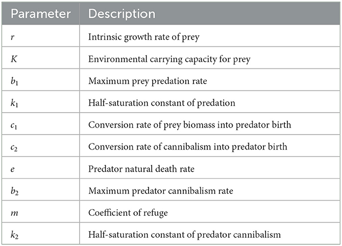
Table 1. Description of parameters.

The value of Equation (2) monotonically increases with the supremum b₂. (1 − m)P is the amount of the available predator to be cannibalized, as m is the coefficient of refuge. The conversion rate of cannibalism into predator birth (c₂) is assumed to be less than the maximum predator cannibalism rate (b₂).

The model proposed by Rayungsari et al. [21] was constructed in a system of nonlinear differential equations with the first-order derivative, where the change of population density at any time depends on the current population density instantaneously. Whereas in reality, the current condition is also affected by the history of all previous conditions, which is called the memory effect [26]. The phenomenon or systems that have memory and genetic characteristics can be described by a fractional differential system [27]. The definition of fractional-order derivative was first introduced by Liouville [28] motivated by L'Hôpital and Leibniz's critical thinking on derivatives of order $\frac{1}{2}$. Liouville's definition was modified by Riemann by applying a direct generalization of the Cauchy formula and named Riemann–Liouville fractional derivative operator [29]. The fractional-order derivative concept by Liouville and Riemann utilizes Euler's study of fractional integration, which led him to construct the Gamma function as generalization of the factorial concept for fractional numbers [30]. In 1967, Michele Caputo modified the Riemann–Liouville operator so that when solving differential equations, no initial conditions are required. The definition of the modified operator is named by Caputo fractional-order derivative operator. Predator–prey models using Caputo-type fractional derivatives have been widely studied recently [24, 31–33]. Hence, in this article, we modify and analyze the Predator–prey model incorporating predator cannibalism and refuge in Rayungsari et al. [21] by applying the Caputo fractional-order derivative operator.

This article is organized as follows. In Section 2, model development and basic properties are described. The basic properties consist of verification of the non-negativity, existence, uniqueness, and boundedness of solutions of the model. In Section 3, the results of dynamical analysis are presented. The results consist of the existence and stability of equilibrium points. Both local and global stability are investigated, while the analyzed bifurcation is the Hopf bifurcation. In Section 4, the numerical simulations and intrepretations are carried out to confirm the analytical results. Finally, in Section 5, we draw some concluding remarks.

2. Model development and basic properties

By applying the Caputo fractional-order derivative operator to the left-hand side of system (Equation 1), the model becomes

$\begin{array}{l}{D}_{*}^{\alpha }N=rN\left(1-\frac{N}{K}\right)-\frac{b_{1}NP}{k_1+N}\\ D_{*}^{\alpha }P=\frac{c_{1}NP}{k_1+N}+c_{2}P-eP-\frac{b_2(1-m)P^2}{k_2+(1-m)P},& (3)\end{array}$

with α ∈ ℝ, 0 < α ≤ 1, and $D_{*}^{\alpha }$ is the α-order of Caputo fractional derivative operator defined by $D_{*}^{\alpha }x\left(t\right)=\frac{1}{\Gamma \left(1-\alpha \right)}{\int }_0^t{\left(t-s\right)}^{-\alpha }x\left(s\right)ds$.

Since the variables in the system (Equation 3) represent the population densities, the solution of the system must be non-negative. The solution of system (Equation 3) is guaranteed to be non-negative by the following theorem.

THEOREM 1. All solutions of Equation (3) are non-negative for any initial values $\left(N\left(0\right),P\left(0\right)\right)\in {ℝ}_{+}^2$.

Proof. Since $D_{*}^{\alpha }=N\left(r\left(1-\frac{N}{K}\right)-\frac{b_{1}P}{k_1+N}\right)$, then $D_{*}^{\alpha }N\left(0\right)=0$ if N(0) = 0. $D_{*}^{\alpha }N=0$ means there is no change of prey population density. Consequently, N(t) = 0, ∀t > 0. Then, we prove that if N(0) > 0 then N(t) ≥ 0 for every t > 0. Suppose that the statement is wrong, so there is t^* > 0 such as

$\begin{array}{l}N(t)>0,0\le t<t^{*},\\ N(t)=0,t=t^{*},\\ N(t)<0,t\ge t^{*},& (4)\end{array}$

From Equations (3), (4), we get that $D_{*}^{\alpha }N=0,t=t^{*}.$ Thus, there is no change in the population density of N when t = t^*. From the prior statement, N(t) = 0, t = t^*, so that N(t) = 0, t > t^*. This contradicts the statement that N(t) < 0 for t > t^*. Therefore, N(t) ≥ 0 for all t > 0 is correct. In the same way, it can be proved that P(t) ≥ 0 for every t > 0.

Next, we show the existence and uniqueness of solution of the system (Equation 3) using Theorem 3.7 in Li et al. [34]. Consider a region [0, ∞) × Ω, where $\Omega =\left\{X=\left(N,P\right)\in {ℝ}_{+}^2:c_2<e\right\}$. Then, we denote a mapping F(X) = (F₁(X), F₂(X)), where

$\begin{array}{l}{F}_1(X)=rN\left(1-\frac{N}{K}\right)-\frac{b_{1}NP}{k_1+N},\\ F_2(X)=\frac{c_{1}NP}{k_1+N}+c_{2}P-eP-\frac{b_2(1-m)P^2}{k_2+(1-m)P}.& (5)\end{array}$

For all $X=\left(N,P\right),\overline{X}=\left(\overline{N},\overline{P}\right)\in \Omega$,

$\begin{array}{l}\left|\right|F(X)-F(\overline{X})\left|\right|\le \left|F_1(X)-F_1(\overline{X})\right|+\left|F_2(X)-F_2(\overline{X})\right|\\ =\left|\left[rN\left(1-\frac{N}{K}\right)-\frac{b_{1}NP}{k_1+N}\right]-\left[r\overline{N}\left(1-\frac{\overline{N}}{K}\right)-\frac{b_1\overline{N}\overline{P}}{k_1+\overline{N}}\right]\right|\\ +|\left[\frac{c_{1}NP}{k_1+N}+c_{2}P-eP-\frac{b_2(1-m)P^2}{k_2+(1-m)P}\right]\\ -\left[\frac{c_1\overline{N}\overline{P}}{k+\overline{N}}+c_2\overline{P}-e\overline{P}-\frac{b_2(1-m){\overline{P}}^2}{k_2+(1-m)\overline{P}}\right]|\\ \le \left|rN-\overline{N}\right|+\left|\frac{N^2-{\overline{N}}^2}{K}\right|+\left|\frac{b_{1}NP(k_1+\overline{N})-b_1\overline{N}\overline{P}(k_1+N)}{(k_1+N)(k_1+\overline{N})}\right|\\ +\left|\frac{c_{1}NP(k_1+\overline{N})-c_1\overline{N}\overline{P}(k_1+N)}{(k_1+N)(k_1+\overline{N})}\right|+\left|(c_2-e)(P-\overline{P})\right|\\ +\left|\frac{b_2(1-m)(P^2(k_2+(1-m)\overline{P})-({\overline{P}}^2(k_2+(1-m)P)}{(k_2+(1-m)P)(k_2+(1-m)\overline{P})}\right|\\ \le \left[r+\frac{r(N+\overline{N})}{K}+\frac{(b_1+c_1)k_{1}P}{(k_1+N)(k_1+\overline{N})}\right]\left|N-\overline{N}\right|\\ +[\frac{(b_1+c_1)\overline{N}}{k_1+\overline{N}}+e-c_2\\ +\frac{b_2(1-m)\left[k_2(P+\overline{P})+P\overline{P}(1-m)\right]}{(k_2+(1-m)P)(k_2+(1-m)\overline{P})}]\left|P-\overline{P}\right|.\end{array}$

Since in the following discussion, it can be proved that the system solution (Equation 3) is bounded in Ω, there is a positive constant M = max{N, P}, ∀t ≥ 0. Hence, we have

$\begin{array}{l}\left|\right|F(X)-F(\overline{X})\left|\right|\le \left[r+\frac{2M}{K}+\frac{(b_1+c_1)k_{1}M}{k_1^2}\right]\left|N-\overline{N}\right|\\ +\left[\frac{(b_1+c_1)M}{k_1}+e-c_2+\frac{b_2(1-m)\left[2k_{2}M+(1-m)M^2\right]}{k_2^2}\right]\\ \left|P-\overline{P}\right|\\ =L_1\left|N-\overline{N}\right|+L_2\left|P-\overline{P}\right|,\end{array}$

with

$\begin{array}{l}{L}_1=r+\frac{2M}{K}+\frac{(b_1+c_1)k_{1}M}{k_1^2},\\ L_2=\frac{(b_1+c_1)M}{k_1}+e-c_2+\frac{b_2(1-m)\left[2k_{2}M+(1-m)M^2\right]}{k_2^2}.\end{array}$

By choosing a positive constant L = max {L₁, L₂}, we get

$\begin{array}{ll}\left|\right|F(X)-F(\overline{X})\left|\right|\le L\left|\right|X-\overline{X}\left|\right|.& (6)\end{array}$

Based on Equation (6), the function F(X) satisfies the Lipschitz condition so that there exist a unique solution X(t) of the system (Equation 3) with any initial value of X(0) = (N(0), P(0)). Thus, we derive the following theorem.

THEOREM 2. For the system (Equation 3) with any non-negative initial condition (N(0), P(0)) ∈ Ω, there exist a unique solution X(t) ∈ Ω.

Next, due to the limited carrying capacity of the prey and predator resources, the size of both populations in the system (Equation 3) must be limited. Consider a function defined by

$V(t)=N(t)+\frac{b_1}{c_1}P(t).$

The Caputo derivative α-order of V satisfies,

$\begin{array}{l}{D}_{*}^{\alpha }V\le D_{*}^{\alpha }N+\frac{b_1}{c_1}{D}_{*}^{\alpha }P\\ =\left[rN\left(1-\frac{N}{K}\right)-\frac{b_{1}NP}{k_1+N}\right]\\ +\frac{b_1}{c_1}\left[\frac{c_{1}NP}{k_1+N}+c_{2}P-eP-\frac{b_2(1-m)P^2}{k_2+(1-m)P}\right]\\ =rN-\frac{r}{K}{N}^2+\frac{b_1}{c_1}\left(c_2-e-\frac{b_2(1-m)P}{k_2+(1-m)P}\right)P\\ \le rN-\frac{r}{K}{N}^2+\frac{b_1}{c_1}\left(c_2-e\right)P.\end{array}$

For any positive constant φ,

$\begin{array}{l}{D}_{*}^{\alpha }V+\phi V\le rN-\frac{r}{K}{N}^2+\frac{b_1}{c_1}(c_2-e)P+\phi \left(N+\frac{b_1}{c_1}P\right)\\ =(r+\phi )N-\frac{r}{K}{N}^2+\frac{b_1}{c_1}(c_2-e+\phi )P.\end{array}$

If c₂ < e and by choosing 0 < φ < e − c₂, we get

$\begin{array}{l}{D}_{*}^{\alpha }V+\phi V<(r+\phi )N-\frac{r}{K}{N}^2\\ =-\frac{r}{K}\left[{\left(N-\frac{(r+\phi )K}{2r}\right)}^2-{\left(\frac{(r+\phi )K}{2r}\right)}^2\right]\\ \le \frac{r}{K}{\left(\frac{(r+\phi )K}{2r}\right)}^2.& (7)\end{array}$

Based on Equation (7), Generalized Mean Value Theorem in Odibat and Shawagfeh [35], and Lemma 6.1 (Fractional Comparison Principle) in Li et al. [34], we get that,

$\begin{array}{l}V(t)\le \left(V(0)-\frac{r}{\phi K}{\left(\frac{(r+\phi )K}{2r}\right)}^2\right)E_{\alpha }\left[-\phi {\left(t\right)}^{\alpha }\right]\\ +\frac{r}{\phi K}{\left(\frac{(r+\phi )K}{2r}\right)}^2.& (8)\end{array}$

$E_{\alpha }\left[-\phi {\left(t\right)}^{\alpha }\right]\to 0ast\to +\infty$, so that,

$V(t)\to \frac{r}{\phi K}{\left(\frac{(r+\phi )K}{2r}\right)}^2,t\to +\infty .$

Hence, we establish the following theorem.

THEOREM 3. All solutions of Equation (2) with initial values $\left(N\left(0\right),P\left(0\right)\right)\in \left\{\left(x,y\right)\in R_{+}^2:c_2<e\right\}$ are uniformly bounded

3. Dynamical analysis

3.1. Existence of equilibrium points

In the similar way as in Rayungsari et al. [21], the system (Equation 3) has four equilibrium points, namely E₀ = (0, 0), E₁ = (0, P₁), E₂ = (K, 0), and E₃ = (N₃, P₃), where $P_1=\frac{k_2\left(e-c_2\right)}{\left(c_2-e-b_2\right)\left(1-m\right)}$. If b₂ + e ≠ c₁ + c₂, then N₃ and P₃ in E₃ is obtained from the solution of a cubic equation using the Cardano's formula [36, 37], i.e.,

$\begin{array}{l}{N}_3=\frac{\sqrt[3]{q_2\pm \sqrt{q_2^2+\frac{4}{27}{q}_1^3}}}{\sqrt[3]{2}}-\frac{q_1\sqrt[3]{2}}{3\sqrt[3]{q_2\pm \sqrt{q_2^2+\frac{4}{27}{q}_1^3}}}-\frac{B}{3A},\\ P_3=\frac{r}{b_1}\left(1-\frac{N_3}{K}\right)(k_1+N_3),& (9)\end{array}$

with

$\begin{array}{l}{q}_1=\frac{3AC-B^2}{3A^2},\\ q_2=\frac{9ABC-2B^3-27A^{2}D}{27A^3},\\ A=\frac{r}{b_{1}K}(1-m)(b_2-c_1-c_2+e),\\ B=\frac{r}{b_1}(1-m)\left[(c_1+c_2-e-b_2)-\frac{k_1}{K}(c_1+2(c_2-e-b_2))\right],\\ C=(c_1+c_2-e)k_2\\ +\frac{r{k}_1}{b_1}(1-m)\left[c_1+(2-k_1)(c_2-e)-2b_2+\frac{b_2{k}_1}{K}\right],\\ D=k_1\left[k_2(c_2-e)+\frac{r{k}_1}{b_1}(1-m)(c_2-e-b_2)\right].\end{array}$

Whereas, if b₂ + e = c₁ + c₂, we have the value of N₃ and P₃ as follows:

$N_3=\frac{-R\pm \sqrt{R^2-4QS}}{2Q},P_3=\frac{r}{b_1}\left(1-\frac{N_3}{K}\right)(k_1+N_3),$

with

$\begin{array}{l}Q=\frac{c_{1}r{k}_1}{b_{1}K}(1-m),\\ R=b_2{k}_2+\frac{r{k}_1}{b_1}(1-m)\left(k_1(c_1-b_2)-c_1+\frac{b_2{k}_1}{K}\right),\\ S=k_1\left[k_2(b_2-c_1)-\frac{r{c}_1{k}_1}{b_1}(1-m)\right].\end{array}$

Two of the equilibrium points need existence conditions. E₁ exists in ${ℝ}_{+}^2$ if 0 < c₂ − e < b₂. The coexistence point E₃ exists in ${ℝ}_{+}^2$ if $q_2^2+\frac{4}{27}{q}_1^3\ge 0$ and 0 < N₃ < K for b₂ + e ≠ c₁ + c₂. Meanwhile, for b₂ + e = c₁ + c₂, E₃ exists in ${ℝ}_{+}^2$ if R² − 4QS ≥ 0 and 0 < N₃ < K.

3.2. Local stability

Local stability of the equilibrium points of Equation (3) are determined by the arguments of the eigenvalues of Jacobian matrix and applying Matignon Local Stability Theorem in Petras [38]. Suppose that E^* is an equilibrium point of system (Equation 3). Based on Matignon Local Stability Theorem, E^* is local asymptotically stable if all of the eigenvalues λ_j of the Jacobian matrix,

$\begin{array}{ll}J(E^{*})=\left[\begin{array}{l}r\left(1-\frac{2N}{K}\right)-\frac{b_1{k}_{1}P}{{(k_1+N)}^2}-\frac{b_{1}N}{k_1+N}\\ \frac{c_1{k}_{1}P}{{(k_1+N)}^2}\frac{c_{1}N}{k_1+N}+c_2-e\\ -\frac{b_2(1-m)P\left[2k_2+(1-m)P\right]}{{(k_2+(1-m)P)}^2}\end{array}\right]& (10)\end{array}$

that satisfies $|arg\left({\lambda }_j\right)|>\frac{\alpha \pi }{2}$.

THEOREM 4. The origin point E₀(0, 0) is always unstable.

Proof. The Jacobian matrix for E₀ = (0, 0) is

$\begin{array}{ll}J\left(E_0\right)=\left[\begin{array}{cc}r& 0\\ 0& c_2-e\end{array}\right],& (11)\end{array}$

so the eigenvalues are λ₁ = r and λ₂ = c₂ − e. The argument of the first eigenvalue is $|arg\left({\lambda }_1\right)|=0<\frac{\alpha \pi }{2}$. If c₂ > e then $|arg\left({\lambda }_2\right)|=0<\frac{\alpha \pi }{2}$ (E₀ is an unstable source), while if c₂ > e then $|arg\left({\lambda }_2\right)|=\pi >\frac{\alpha \pi }{2}$ (E₀ is an unstable saddle node).

THEOREM 5. Prey extinction point E₁ (0, P₁) is local asymptotically stable if $r<\frac{b_1{P}_1}{k_1}$ and unstable saddle node if $r>\frac{b_1{P}_1}{k_1}$.

Proof. By substituting E₁ = (0, P₁) to Equation (10), we get the Jacobian matrix for E₁,

$\begin{array}{ll}J\left(E_1\right)=\left[\begin{array}{cc}r-\frac{b_1{P}_1}{k_1}& 0\\ \frac{c_1{P}_1}{k_1}& \frac{(c_2-e)(c_2-e-b_2)}{b_2}\end{array}\right].& (12)\end{array}$

The eigenvalues are ${\lambda }_1=r-\frac{b_1{P}_1}{k_1}$ and ${\lambda }_2=\frac{\left(c_2-e\right)\left(c_2-e-b_2\right)}{b_2}$. Based on the existence condition of E₁, then λ₂ is the negative real number and $|arg\left({\lambda }_2\right)|=\pi >\frac{\alpha \pi }{2}$. Hence, the local stability of E₁ depends on λ₁. If $r<\frac{b_1{P}_1}{k_1},$ λ₁ < 0, and $|arg\left({\lambda }_1\right)|=\pi >\frac{\alpha \pi }{2}$ so that E₁ is local asymptotically stable. Otherwise, if $r>\frac{b_1{P}_1}{k_1}$ then λ₁ > 0, $|arg\left({\lambda }_1\right)|=\pi >\frac{\alpha \pi }{2}$, and E₁ is an unstable saddle node.

THEOREM 6. The predator extinction point E₂(K, 0) is local asymptotically stable if $e>\frac{c_{1}K}{k_1+K}+c_2$ and unstable saddle node if $e<\frac{c_{1}K}{k_1+K}+c_2$.

Proof. With the same way, we get the Jacobian matrix for E₂ as follows:

$\begin{array}{ll}J\left(E_2\right)=\left[\begin{array}{cc}-r& -\frac{b_{1}K}{k_1+K}\\ 0& \frac{c_{1}K}{k_1+K}+c_2-e\end{array}\right].& (13)\end{array}$

The eigenvalues are λ₁ = −r and ${\lambda }_2=\frac{c_{1}K}{k_1+K}+c_2-e$. It is clear that $|arg\left({\lambda }_1\right)|=\pi >\frac{\alpha \pi }{2}$. E₂ is local asymptotically stable if $|arg\left({\lambda }_2\right)|>\frac{\alpha \pi }{2}$, i.e., for $e>\frac{c_{1}K}{k_1+K}+c_2$. If $e<\frac{c_{1}K}{k_1+K}+c_2$, $|arg\left({\lambda }_2\right)|=0<\frac{\alpha \pi }{2}$, and E₂ is an unstable saddle node.

For existence point E₃(N₃, P₃), the Jacobian matrix is as follows:

$\begin{array}{ll}J\left(E_3\right)=\left[\begin{array}{cc}{J}_{11}& J_{12}\\ J_{21}& J_{22}\end{array}\right],& (14)\end{array}$

where

$\begin{array}{l}{J}_{11}=\frac{r{N}_3}{k_1+N_3}\left(1-\frac{k_1+2N_3}{K}\right),\\ J_{12}=-\frac{b_1{N}_3}{k_1+N_3},\\ J_{21}=\frac{c_1{k}_{1}r}{b_1(k_1+N_3)}\left(1-\frac{N_3}{K}\right),\\ J_{22}=-\frac{b_1{b}_2{k}_{2}r(1-m)\left(1-\frac{N_3}{K}\right)(k_1+N_3)}{{\left(b_1{k}_2+r(1-m)\left(1-\frac{N_3}{K}\right)(k_1+N_3)\right)}^2}.& (15)\end{array}$

Thus, the eigenvalues are obtained from the following quadratic equation.

$\begin{array}{ll}{\lambda }^2-trace(J(E_3))+\det (J(E_3))=0,& (16)\end{array}$

where

$\begin{array}{l}\det (J(E_3))=J_{11}{J}_{22}-J_{12}{J}_{21}\\ =-\frac{r^2{b}_1{b}_2{k}_2(1-m)N_3\left(1-\frac{N_3}{K}\right)}{{\left(b_1{k}_2+r(1-m)\left(1-\frac{N_3}{K}\right)(k_1+N_3)\right)}^2}\left(1-\frac{k_1+2N_3}{K}\right)\\ +\frac{c_1{k}_{1}r{N}_3}{{(k_1+N_3)}^2}\left(1-\frac{N_3}{K}\right)& (17)\end{array}$

and

$\begin{array}{l}trace(J(E_3))=J_{11}+J_{22}\\ =\frac{r{N}_3}{k_1+N_3}\left(1-\frac{k_1+2N_3}{K}\right)\\ -\frac{b_1{b}_2{k}_{2}r(1-m)\left(1-\frac{N_3}{K}\right)(k_1+N_3)}{{\left(b_1{k}_2+r(1-m)\left(1-\frac{N_3}{K}\right)(k_1+N_3)\right)}^2}.& (18)\end{array}$

Suppose that

$\begin{array}{ll}a=\frac{b_1{b}_2{k}_2(1-m)\left(1-\frac{N_3}{K}\right){(k_1+N_3)}^2}{N_3{\left(b_1{k}_2+r(1-m)\left(1-\frac{N_3}{K}\right)(k_1+N_3)\right)}^2}>0,& (19)\end{array}$

then

$\begin{array}{l}trace(J(E_3))=\frac{r{N}_3}{k_1+N_3}\left(1-\frac{k_1+2N_3}{K}\right)-\frac{ar{N}_3}{k_1+N_3}\\ =\frac{r{N}_3}{k_1+N_3}\left(1-a-\frac{k_1+2N_3}{K}\right)\\ =\frac{r{N}_3}{k_1+N_3}\left(\frac{K-aK-k_1-2N_3}{K}\right).& (20)\end{array}$

Suppose that d is the discriminant of Equation (16), i.e.,

$\begin{array}{ll}d=trace{\left(J\left(E_3\right)\right)}^2-4\text{ det}\left(J\left(E_3\right)\right).& (21)\end{array}$

The cases are divided into two parts, those are for d ≥ 0 and for d < 0.

1. Case 1 (d ≥ 0)

For this case, if k₁ > K − 2N₃, we have det(J) > 0 and trace(J) < 0. Therefore, the eigenvalues (solutions of Equation 16) are real and negative. Consequently, $|arg\left({\lambda }_j\right)|=\pi >\frac{\alpha \pi }{2}$ for j = 1, 2 and E₃ is local asymptotically stable.

2. Case 2 (d < 0)

In case (d < 0), the eigenvalues are complex number with non-zero imaginary part $\lambda =\frac{trace\left(J\left(E_3\right)\right)+\sqrt{d}}{2}$ and $\overline{\lambda }=\frac{trace\left(J\left(E_3\right)\right)-\sqrt{d}}{2}$. Suppose that

(a) If k₁ > K − 2N₃ − aK, then trace(J) < 0 so that Re(λ) < 0 and E₃ is local asymptotically stable since $|arg\left(\lambda \right)|=|arg\left(\overline{\lambda }\right)|=\pi >\frac{\alpha \pi }{2}$.

(b) If k₁ < K − 2N₃ − aK, then trace(J) > 0 so that Re(λ) > 0 and E₃ is local asymptotically stable if $|arg\left(\lambda \right)|>\frac{\alpha \pi }{2}$.

Hence, we establish the following theorem.

THEOREM 7. Suppose that $d=trace{\left(J\left(E_3\right)\right)}^2-4\text{ det}\left(J\left(E_3\right)\right)$ with trace(J(E₃)) and det(J(E₃)) are the trace and determinant of matrix J(E₃) in Equation (14). E₃ = (N₃, P₃) is locally asymptotically stable if one of the following conditions are satisfied.

1. d ≥ 0 and k₁ > K − 2N₃,

2. d < 0 and k₁ > K − 2N₃ − aK,

3. d < 0, k₁ < K − 2N₃ − aK, and $|arg\left(\lambda \right)|=\left|\frac{Im\left(\lambda \right)}{Re\left(\lambda \right)}\right|=\left|\frac{\lambda -\overline{\lambda }}{\lambda +\overline{\lambda }}\right|>\frac{\alpha \pi }{2}$,

with a is as in Equation (19).

3.3. Global stability

Next, we investigate the global stability of E₁, E₂, and E₃. For this aim, we use the help of Lemma 3.1 in Vargas-De-Leon [39] and Generalized Lasalle Invariance Principle in Huo et al. [40].

For prey extinction point E₁(0, P₁), we consider a Lyapunov function,

$V_1(N,P)=N+\frac{b_1}{c_1}\left(P-P_1-P_1\ln \frac{P}{P_1}\right).$

The Caputo derivative α-order of V₁ is as follows:

$\begin{array}{l}{D}_{*}^{\alpha }{V}_1\le D_{*}^{\alpha }N+\frac{b_1}{c_1}\left(\frac{P-P_1}{P}\right)D_{*}^{\alpha }P\\ =rN\left(1-\frac{N}{K}\right)-\frac{b_{1}NP}{k_1+N}\\ +\frac{b_1}{c_1}\left(\frac{P-P_1}{P}\right)\left(\frac{c_{1}NP}{k_1+N}+c_{2}P-eP-\frac{b_2(1-m)P^2}{k_2+(1-m)P}\right)\\ =rN\left(1-\frac{N}{K}\right)-\frac{b_{1}N{P}_1}{k_1+N}\\ +\frac{b_1}{c_1{P}_1}\left(P-P_1\right)\left(\frac{k_2(c_2-e)P_1+k_2(e-c_2)P}{k_2+(1-m)P}\right)\\ =rN\left(1-\frac{N}{K}\right)-\frac{b_{1}N{P}_1}{k_1+N}\\ -\frac{b_1}{c_1{P}_1}{\left(P-P_1\right)}^2\left(\frac{k_2(c_2-e)}{k_2+(1-m)P}\right)\\ \le rN\left(1-\frac{N}{K}\right)-\frac{b_{1}N{P}_1}{k_1+N}.\end{array}$

If $r<\frac{b_1{P}_1}{k_1}$, then we have,

$\begin{array}{l}{D}_{*}^{\alpha }{V}_1\le rN\left(1-\frac{N}{K}\right)-\frac{r{k}_{1}N}{k_1+N}\\ =\frac{rN}{K(k_1+N)}\left(KN-k_{1}N-N^2\right).\end{array}$

$D_{*}^{\alpha }{V}_1=0$ only if N = 0. For N > 0, if K ≤ k₁, then $D_{*}^{\alpha }{V}_1\le 0$ and according to Generalized Lasalle Invariance Principle [40], E₁ is globally asymptotically stable. We write the global stability conditions of E₁ in the following theorem.

THEOREM 8. If E₁ = (0, P₁) exists, then E₁ is globally asymtotically stable if $r<\frac{b_1{P}_1}{k_1}$ and K ≤ k₁.

Then, we construct a Lyapunov function as follows:

$V_2(N,P)=\frac{c_1}{b_1}\left(N-K-K\ln \frac{N}{K}\right)+P,$

for E₂(K, 0). We have,

$\begin{array}{l}{D}_{*}^{\alpha }{V}_2\le \frac{c_1}{b_1}\left(\frac{N-K}{N}\right)D_{*}^{\alpha }N+D_{*}^{\alpha }P\\ =\frac{c_1}{b_1}\left(\frac{N-K}{N}\right)\left(rN\left(1-\frac{N}{K}\right)-\frac{b_{1}NP}{k_1+N}\right)+\frac{c_{1}NP}{k_1+N}\\ +c_{2}P-eP-\frac{b_2(1-m)P^2}{k_2+(1-m)P}\\ =-\frac{c_{1}r}{b_{1}K}{\left(N-K\right)}^2\\ +P\left(\frac{c_{1}K}{k_1+N}+c_2-e-\frac{b_2(1-m)P}{k_2+(1-m)P}\right)\\ \le P\left(\frac{c_{1}K}{k_1+N}+c_2-e-\frac{b_2(1-m)P}{k_2+(1-m)P}\right)\\ \le P\left(\frac{c_{1}K}{k_1+N}+c_2-e\right).\end{array}$

Suppose that $e>\frac{c_{1}K}{k_1}+c_2$. Thus, we have,

$\begin{array}{l}{D}_{*}^{\alpha }{V}_2\le P\left(\frac{c_{1}K}{k_1+N}+c_2-\left(\frac{c_{1}K}{k_1}+c_2\right)\right)\\ =P\left(\frac{c_{1}K}{k_1+N}-\frac{c_{1}K}{k_1}\right)\le 0.\end{array}$

We get that $D_{*}^{\alpha }{V}_2\le 0,\forall \left(N,P\right)\in {ℝ}_{+}^2$. Hence, E₂ is globally asymptotically stable with the condition as in the following theorem.

THEOREM 9. E₂ is globally asymtotically stable if $e>\frac{c_{1}K}{k_1}+c_2$.

To investigate the global stability of coexistence point, we consider a Lyapunov function

$V_3(N,P)=N-N_3-N_3\ln \frac{N}{N_3}+\frac{b_1}{c_1}\left(P-P_3-P_3\ln \frac{P}{P_3}\right),$

where N₃ and P₃ as in Equation (9). The α-order derivative of V₃ satisfies

$\begin{array}{l}{D}_{*}^{\alpha }{V}_3\le \left(1-\frac{N_3}{N}\right)\left(rN\left(1-\frac{N}{K}\right)-\frac{b_{1}NP}{k_1+N}\right)\\ +\frac{b_1}{c_1}\left(1-\frac{P_3}{P}\right)\left(\frac{c_{1}NP}{k_1+N}+c_{2}P-eP-\frac{b_2(1-m)P^2}{k_2+(1-m)P}\right)\\ =\left(N-N_3\right)\left[r\left(\frac{N_3-N}{K}\right)-\frac{b_1{k}_1(P-P_3)}{(k_1+N)(k_1+N_3)}\right]\\ +\frac{b_1}{c_1}\left(P-P_3\right)[\frac{c_1{k}_1(N-N_3)}{(k_1+N)(k_1+N_3)}\\ -\frac{b_2{k}_2(1-m)(P-P_3)}{(k_2+(1-m)P)(k_2+(1-m)P_3)}]\\ =-\frac{r}{K}{\left(N-N_3\right)}^2-\frac{b_1(N-N_3)(N_{3}P-N{P}_3)}{(k_1+N)(k_1+N_3)}\\ -\frac{b_1{b}_2{k}_2(1-m){(P-P_3)}^2}{c_1(k_2+(1-m)P)(k_2+(1-m)P_3)}.\end{array}$

Consider a domain ${\Omega }^{*}=\left\{\left(N,P\right)|\frac{P}{P_3}>\frac{N}{N_3}>1\right\}$. Then, $D_{*}^{\alpha }{V}_3<0$ and E₃ is globally asymptotically stable in Ω^*. Hence, we derive the following theorem.

THEOREM 10. E₃ is globally asymptotically stable in the domain ${\Omega }^{*}=\left\{\left(N,P\right)|\frac{P}{P_3}>\frac{N}{N_3}>1\right\}.$

3.4. Existence of Hopf bifurcation

THEOREM 11. If d < 0 and k₁ < K − 2N₃ − aK with a is given in Equation (19), then E₃ undergoes Hopf bifurcation when the order of Caputo derivative, α, pass α^* with

$\begin{array}{ll}{\alpha }^{*}={\tan }^{-1}\left|\frac{Im({\lambda }^{*})}{Re({\lambda }^{*})}\right|& (22)\end{array}$

and λ^* is an eigenvalue of E₃.

Proof. Suppose that d < 0 and k₁ < K − 2N₃ − aK. Then, the eigenvalues of J(E₃) are a pair of complex number ${\lambda }_1={\lambda }^{*}$ and ${\lambda }_2=\overline{{\lambda }^{*}}$ with positive real part. Suppose that

$f(\alpha )=\frac{\alpha \pi }{2}-\min \left|\arg {\left({\lambda }_i\right)}_{i=1,2}\right|.$

For α = α^* with

${\alpha }^{*}={\tan }^{-1}\left|\frac{Im({\lambda }^{*})}{Re({\lambda }^{*})}\right|,$

we have f(α^*) = 0 and ${\frac{df\left(\alpha \right)}{d\alpha }|}_{\alpha ={\alpha }_{*}}=\frac{\pi }{2}\ne 0$. According to Theorem 3 in Li and Wu [41], E₃ undergoes Hopf bifurcation at α = α^*.

4. Numerical simulations

In this section, numerical simulations of the model (Equation 3) are carried out using Matlab software and the predictor–corrector scheme, which is introduced by Diethelm et al. [42]. The purposes of the numerical simulations are to confirm the dynamics analysis results and the existence of Hopf bifurcation. Since there are no available data related to our proposed model yet, the parameter values are chosen hypothetically in Table 2.

TABLE 2

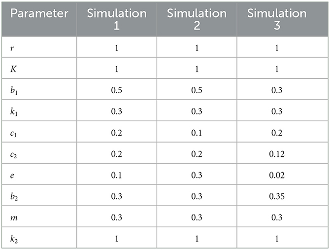
Table 2. Parameter values.

For parameter values in Simulation 1, E₁ exists, i.e., E₁ = (0, 0.7143) and the local stability condition in Theorem 5 is satisfied. We conduct numerical simulations with several values of α. The results in Figure 1 show that the solutions tend to the prey extinction point for all α values chosen. This is consistent with the analytical results since the Jacobi matrix eigenvalues are negative real numbers, which involve E₁ always asymptotically stable with the selected parameter values for any order derivative of the α ∈ (0, 1]. However, we can see a difference in the solution's behavior for each α. The lower the α value, the slower the solution reaches E₁.

FIGURE 1

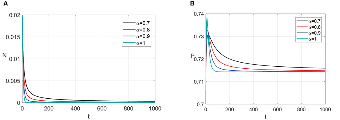
Figure 1. Graphic solutions of Simulation 1. (A) Solutions of N with respect to time t. (B) Solutions of P with respect to time t.

For the second simulation, we use the same parameter values but c₁ and e (see Table 2). As a result, the existence condition for E₁ is not satisfied, so the point does not exist. It means that the prey can survive from extinction. For the predator extinction point E₂(1, 0), the stability condition in Theorem 6 is satisfied and E₂ is asymptotically stable for any fractional order of α ∈ (0, 1]. It fits the numerial simulation results in Figure 2. Represented by some values of α, we can see that the solutions with initial value close to E₂ go to E₂. With a greater α value, the solution will reach the predator extinction point faster.

FIGURE 2

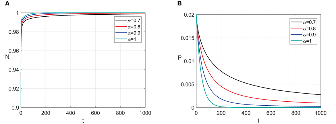
Figure 2. Graphic solutions of Simulation 2. (A) Solutions of N with respect to time t. (B) Solutions of P with respect to time t.

Next, we demonstrate the effect of the derivative order on the behavior of the solution, with 0.8 ≤ α ≤ 1. The parameter values in the last column of Table 2 were chosen. With those parameter values, the coexistence point exists, i.e., E₃(0.1423, 1.2645), which has the eigenvalues λ^* = 0.0232 + 0.1589i and $\overline{{\lambda }^{*}}=0.0232-0.1589i$. The parameter values satisfy k₁ < K − 2N₃ − aK and the discriminant of the quadratic equation of the eigenvalues is negative, i.e., d = −0.1010. Based on the Theorem 7, the stability of E₃ is determined by the argument of the order derivative α. The threshold is α^* = 0.9077, which satisfies ${\alpha }^{*}<\frac{2}{\pi }\left|\frac{{\lambda }^{*}-\overline{{\lambda }^{*}}}{{\lambda }^{*}+\overline{{\lambda }^{*}}}\right|$.

From the bifurcation diagram in Figure 3, we can see that for α < α^*, the solutions tend to E₃. Meanwhile, for α > α^*, the solutions tend to limit cycle around E₃. As confirmation of the bifurcation diagram, two α values satisfying α < α^*, i.e., α = 0.8 and α = 0.89, and two α values satisfying α.α^*, i.e., α = 0.91 and α = 1, are selected to simulate the solutions of N and P with respect to time. For α = 0.8 and α = 0.89, the solutions tend to E₃. The solution with α = 0.89 oscillates longer than α = 0.8 before finally convergent to E₃. Meanwhile, for α = 0.91 and α = 1, each solution convergent to a limit cycle. The amplitude of the limit cycle solution with α = 1 is greater than α = 0.91.

FIGURE 3

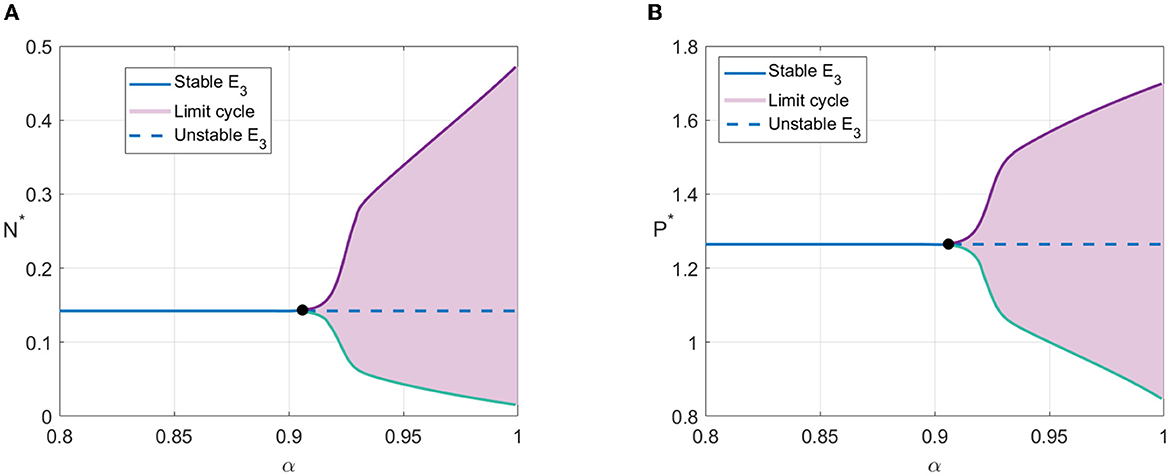
Figure 3. Bifurcation diagram with α as bifurcation parameter. (A) Value of N^* with respect to derivative order α. (B) Value of P^* with respect to derivative order α.

Numerical simulations in Figures 3, 4 show the existence of Hopf bifurcation in system (3) with α as bifurcation parameter. In addition, the system also undergoes one-parameter Hopf bifurcation with other bifurcation parameters such as cannibalism rate (b₂) and refuge coefficient (m). The bifurcation diagrams are shown in Figures 5, 6, respectively.

FIGURE 4

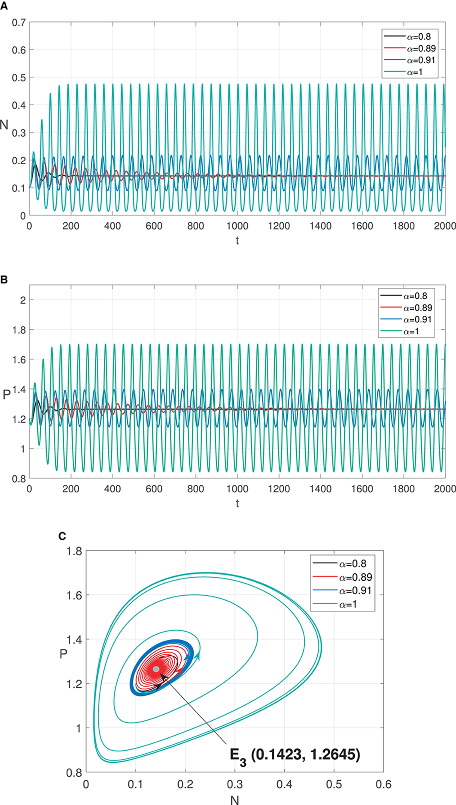
Figure 4. Graphic solutions of Simulation 3. (A) Solutions of N with respect to time t. (B) Solutions of P with respect to time t. (C) Phase portraits.

FIGURE 5

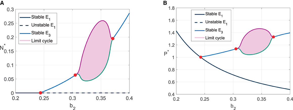
Figure 5. Bifurcation diagram with b₂ as bifurcation parameter. (A) The value of N^* for 0.2 ≤ b₂ ≤ 0.4. (B) The value of P^* for 0.2 ≤ b₂ ≤ 0.4.

FIGURE 6

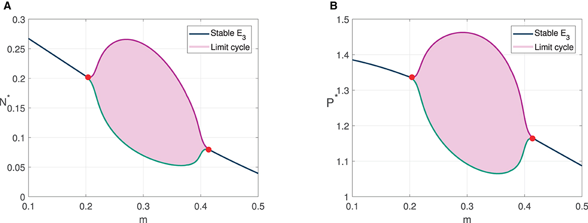
Figure 6. Bifurcation diagram with m as bifurcation parameter. (A) The value of N^* for 0.1 ≤ m ≤ 0.5. (B) The value of P^* for 0.1 ≤ m ≤ 0.5.

For bifurcation diagram with parameter b₂, we have three bifurcation points, i.e., $b_2^{*}=0.2429$, $b_2^{**}=0.306$, and $b_2^{***}=0.372$. For $b_2<b_2^{*}$, the solutions convergent to prey extinction point E₁. It is in accordance with the analytical result since the stability condition of E₁ is satisfied. When the predator cannibalism rate is increased pass $b_2^{*}$, E₁ is unstable, and the solutions convergent to the coexistence point, which means the predator survive from extinction. The solutions tend to limit cycle when $b_2^{**}<b_2<b_2^{***}$. For bifurcation diagram with parameter m, we have two bifurcation points, i.e., m^*, m^**. For m < m^*, the solutions convergent to coexistence point. The solutions tend to limit cycle in the refuge coefficient range m^* < m < m^**.

5. Conclusion

A first-order system of Predator–prey interaction incorporating predator cannibalism and refuge is modified by applying Caputo fractional-order derivative operator. We verify the non-negativity, existence, uniqueness, and boundedness of the model solution. The local and global stability of equilibrium points are then examined. In addition, the existence of Hopf bifurcation is investigated. There are four equilibrium points in the model: the origin point, the prey extinction point, the predator extinction point, and the coexistence point. Since the eigenvalues are real numbers, the first three equilibrium points have the same local stability as the first-order system. However, the local stability of the coexistence point differs from that of the first-order system. The coexistence point with positive real-part eigenvalues is locally asymptotically stable in the modified system as long as the absolute of the eigenvalue arguments are bigger than $\frac{\alpha \pi }{2}$. Even though it is based on different theories, the global stability properties of all equilibrium points are identical to those in the first-order system. Under certain conditions, the Hopf bifurcation exists for the coexistence point. Numerical simulations confirmed the analytical results of stability properties and the existence of Hopf bifurcation.

Data availability statement

The original contributions presented in the study are included in the article/supplementary material, further inquiries can be directed to the corresponding author.

Author contributions

AS and WMK: conceptualization. MR, AS, and ID: methodology. MR: software, data curation, writing—original draft preparation, and visualization. AS, WMK, and ID: validation, writing—reviewing and editing, and supervision. MR and AS: formal analysis. MR, AS, WMK, and ID: investigation. AS: resources and project administration. All authors have read and agreed to the published version of the manuscript.

Conflict of interest

The authors declare that the research was conducted in the absence of any commercial or financial relationships that could be construed as a potential conflict of interest.

Publisher's note

All claims expressed in this article are solely those of the authors and do not necessarily represent those of their affiliated organizations, or those of the publisher, the editors and the reviewers. Any product that may be evaluated in this article, or claim that may be made by its manufacturer, is not guaranteed or endorsed by the publisher.

References

1. Djilali S, Bentout S. Spatiotemporal patterns in a diffusive predator-prey model with prey social behavior. Acta Appl Math. (2020) 169:125–43. doi: 10.1007/s10440-019-00291-z

CrossRef Full Text | Google Scholar

2. Mezouaghi A, Djilali S, Bentout S, Biroud K. Bifurcation analysis of a diffusive predator-prey model with prey social behavior and predator harvesting. Math Methods Appl Sci. (2022) 45:718–31. doi: 10.1002/mma.7807

CrossRef Full Text | Google Scholar

3. Beay LK, Suryanto A, Darti I, et al. Hopf bifurcation and stability analysis of the Rosenzweig-MacArthur predator-prey model with stage-structure in prey. Math Biosci Eng. (2020) 17:4080–97. doi: 10.3934/mbe.2020226

PubMed Abstract | CrossRef Full Text | Google Scholar

4. Bentout S, Djilali S, Atangana A. Bifurcation analysis of an age-structured prey-predator model with infection developed in prey. Math Methods Appl Sci. (2022) 45:1189–208. doi: 10.1002/mma.7846

CrossRef Full Text | Google Scholar

5. Rayungsari M, Kusumawinahyu WM, Marsudi M. Dynamical analysis of predator-prey model with ratio-dependent functional response. Appl Math Sci. (2014) 8:1401–10. doi: 10.12988/ams.2014.4111

PubMed Abstract | CrossRef Full Text | Google Scholar

6. Blyuss KB, Kyrychko YN, Blyuss OB. Complex dynamics near extinction in a predator-prey model with ratio dependence and Holling type III functional response. Front Appl Math Stat. (2022) 2022:123. doi: 10.3389/fams.2022.1083815

CrossRef Full Text

7. Suryanto A, Darti I, S Panigoro H, Kilicman A. A fractional-order predator-prey model with ratio-dependent functional response and linear harvesting. Mathematics. (2019) 7:1100. doi: 10.3390/math7111100

CrossRef Full Text | Google Scholar

8. Panigoro HS, Rahmi E, Resmawan R. Bifurcation analysis of a predator-prey model involving age structure, intraspecific competition, Michaelis-Menten type harvesting, and memory effect. Front Appl Mathand Statistics. (2023) 2023:124. doi: 10.3389/fams.2022.1077831

CrossRef Full Text

9. Trapanese C, Bey M, Tonachella G, Meunier H, Masi S. Prolonged care and cannibalism of infant corpse by relatives in semi-free-ranging capuchin monkeys. Primates. (2020) 61:41–47. doi: 10.1007/s10329-019-00747-8

PubMed Abstract | CrossRef Full Text | Google Scholar

10. Oliva-Vidal P, Tobajas J, Margalida A. Cannibalistic necrophagy in red foxes: do the nutritional benefits offset the potential costs of disease transmission? Mammalian Biol. (2021) 101:1115–20. doi: 10.1007/s42991-021-00184-5

CrossRef Full Text | Google Scholar

11. Allen ML, Krofel M, Yamazaki K, Alexander EP, Koike S. Cannibalism in bears. Ursus. (2022) 2022:1–9. doi: 10.2192/URSUS-D-20-00031.2

CrossRef Full Text | Google Scholar

12. Cunha-Saraiva F, Balshine S, Wagner RH, Schaedelin FC. From cannibal to caregiver: tracking the transition in a cichlid fish. Animal Behaviour. (2018) 139:9–17. doi: 10.1016/j.anbehav.2018.03.003

CrossRef Full Text | Google Scholar

13. Canales TM, Delius GW, Law R. Regulation of fish stocks without stock-recruitment relationships: the case of small pelagic fish. Fish Fish. (2020) 21:857–71. doi: 10.1111/faf.12465

CrossRef Full Text | Google Scholar

14. Koltz AM, Wright JP. Impacts of female body size on cannibalism and juvenile abundance in a dominant arctic spider. J Animal Ecol. (2020) 89:1788–98. doi: 10.1111/1365-2656.13230

PubMed Abstract | CrossRef Full Text | Google Scholar

15. Marchetti MF, Persons MH. Egg sac damage and previous egg sac production influence truncated parental investment in the wolf spider, Pardosa milvina. Ethology. (2020) 126:1111–21. doi: 10.1111/eth.13091

CrossRef Full Text | Google Scholar

16. Zhang S, Yu L, Tan M, Tan NY, Wong XX, Kuntner M, et al. Male mating strategies to counter sexual conflict in spiders. Commun Biol. (2022) 5:1–12. doi: 10.1038/s42003-022-03512-8

PubMed Abstract | CrossRef Full Text | Google Scholar

17. Bose APH. Parent-offspring cannibalism throughout the animal kingdom: a review of adaptive hypotheses. Biol Rev. (2022) 97:1868–85. doi: 10.1111/brv.12868

PubMed Abstract | CrossRef Full Text | Google Scholar

18. Kang Y, Rodriguez-Rodriguez M, Evilsizor S. Ecological and evolutionary dynamics of two-stage models of social insects with egg cannibalism. J Math Anal Appl. (2015) 430:324–53. doi: 10.1016/j.jmaa.2015.04.079

CrossRef Full Text | Google Scholar

19. Zhang F, Chen Y, Li J. Dynamical analysis of a stage-structured predator-prey model with cannibalism. Math Biosci. (2019) 307:33–41. doi: 10.1016/j.mbs.2018.11.004

PubMed Abstract | CrossRef Full Text | Google Scholar

20. Deng H, Chen F, Zhu Z, Li Z. Dynamic behaviors of Lotka-Volterra predator-prey model incorporating predator cannibalism. Adv Diff Equat. (2019) 1:359. doi: 10.1186/s13662-019-2289-8

CrossRef Full Text | Google Scholar

21. Rayungsari M, Suryanto A, Kusumawinahyu WM, Darti I. Dynamical analysis of a predator-prey model incorporating predator cannibalism and refuge. Axioms. (2022) 11:116. doi: 10.3390/axioms11030116

CrossRef Full Text | Google Scholar

22. Mondal S, Samanta G. Dynamics of an additional food provided predator-prey system with prey refuge dependent on both species and constant harvest in predator. Physica A. (2019) 534:122301. doi: 10.1016/j.physa.2019.122301

CrossRef Full Text | Google Scholar

23. Saha S, Samanta G. Analysis of a predator-prey model with herd behavior and disease in prey incorporating prey refuge. Int J Biomath. (2019) 12:1950007. doi: 10.1142/S1793524519500074

CrossRef Full Text | Google Scholar

24. Panigoro HS, Rahmi E, Achmad N, Mahmud SL. The influence of additive Allee effect and periodic harvesting to the dynamics of Leslie-Gower predator-prey model. Jambura J Math. (2020) 2:87–96. doi: 10.34312/jjom.v2i2.4566

CrossRef Full Text | Google Scholar

25. Qi H, Meng X. Threshold behavior of a stochastic predator-prey system with prey refuge and fear effect. Appl Math Lett. (2021) 113:106846. doi: 10.1016/j.aml.2020.106846

CrossRef Full Text | Google Scholar

26. Suryanto A, Darti I, Anam S. Stability analysis of a fractional order modified Leslie-Gower model with additive Allee effect. Int J Math Math Sci. (2017) 2017:1–9. doi: 10.1155/2017/8273430

CrossRef Full Text | Google Scholar

27. Li Z, Liu L, Dehghan S, Chen Y, Xue D. A review and evaluation of numerical tools for fractional calculus and fractional order controls. Int J Control. (2017) 90:1165–81. doi: 10.1080/00207179.2015.1124290

CrossRef Full Text | Google Scholar

28. Liouville J. Memoire Sur Le Calcul Des Differentielles a Indices Quelconques. (1832). Available online at: https://books.google.com/books?id=6jfBtwAACAAJ

29. Samko SG, Kilbas AA, Marichev OI. Fractional Integrals and Derivatives: Theory and Applications. Switzerland; Philadelphia, PA: Gordon and Breach Science Publishers (1993).

Google Scholar

30. Farid G. A unified integral operator and further its consequences. Open J Math Anal. (2020) 4:1–7. doi: 10.30538/psrp-oma2020.0047

CrossRef Full Text | Google Scholar

31. Panigoro HS, Suryanto A, Kusumawinahyu WM, Darti I. Dynamics of an eco-epidemic predator-prey model involving fractional derivatives with power-law and Mittag-Leffler kernel. Symmetry. (2021) 13:785. doi: 10.3390/sym13050785

CrossRef Full Text | Google Scholar

32. Rahmi E, Darti I, Suryanto A. A modified leslie-gower model incorporating beddington-deangelis functional response, double allee effect and memory effect. Fractal Fract. (2021) 5:84. doi: 10.3390/fractalfract5030084

CrossRef Full Text | Google Scholar

33. Alqhtani M, Owolabi KM, Saad KM. Spatiotemporal (target) patterns in sub-diffusive predator-prey system with the Caputo operator. Chaos Solitons Fractals. (2022) 160:112267. doi: 10.1016/j.chaos.2022.112267

CrossRef Full Text | Google Scholar

34. Li Y, Chen Y, Podlubny I. Stability of fractional-order nonlinear dynamic systems: lyapunov direct method and generalized Mittag-Leffler stability. Comput Math Appl. (2010) 59:1810–21. doi: 10.1016/j.camwa.2009.08.019

CrossRef Full Text | Google Scholar

35. Odibat ZM, Shawagfeh NT. Generalized Taylor's formula. Appl Math Comput. (2007) 186:286–93. doi: 10.1016/j.amc.2006.07.102

CrossRef Full Text | Google Scholar

36. Ganti S, Gopinathan S. A note on the solutions of cubic equations of state in low temperature region. J Mol Liquids. (2020) 315:113808. doi: 10.1016/j.molliq.2020.113808

CrossRef Full Text | Google Scholar

37. Hafsi Z. Accurate explicit analytical solution for Colebrook-White equation. Mech Res Commun. (2021) 111:103646. doi: 10.1016/j.mechrescom.2020.103646

CrossRef Full Text | Google Scholar

38. Petras I. Fractional-order Nonlinear Systems: Modeling, Analysis, and Simulation. Beijing: Springer London (2011).

39. Vargas-De-Leon C. Volterra-type Lyapunov functions for fractional-order epidemic systems. Commun Nonlinear Sci Numer Simulat. (2015) 24:75–85. doi: 10.1016/j.cnsns.2014.12.013

CrossRef Full Text | Google Scholar

40. Huo J, Zhao H, Zhu L. The effect of vaccines on backward bifurcation in a fractional order HIV model. Nonlinear Anal Real World Appl. (2015) 26:289–305. doi: 10.1016/j.nonrwa.2015.05.014

CrossRef Full Text | Google Scholar

41. Li X, Wu R. Hopf bifurcation analysis of a new commensurate fractional-order hyperchaotic system. Nonlinear Dyn. (2014) 78:279–88. doi: 10.1007/s11071-014-1439-5

CrossRef Full Text | Google Scholar

42. Diethelm K, Ford NJ, Freed AD. A predictor-corrector approach for the numerical solution of fractional differential equations. Nonlinear Dyn. (2002) 29:3–22. doi: 10.1023/A:1016592219341

CrossRef Full Text | Google Scholar